The Waldmeier effect and the flux transport solar dynamo

Abstract

We confirm that the evidence for the Waldmeier effect WE1 (the anti-correlation between rise times of sunspot cycles and their strengths) and the related effect WE2 (the correlation between rise rates of cycles and their strengths) is found in different kinds of sunspot data. We explore whether these effects can be explained theoretically on the basis of the flux transport dynamo models of sunspot cycles. Two sources of irregularities of sunspot cycles are included in our model: fluctuations in the poloidal field generation process and fluctuations in the meridional circulation. We find WE2 to be a robust result which is produced in different kinds of theoretical models for different sources of irregularities. The Waldmeier effect WE1, on the other hand, arises from fluctuations in the meridional circulation and is found only in the theoretical models with reasonably high turbulent diffusivity which ensures that the diffusion time is not more than a few years.

1 Introduction

Waldmeier (1935) noted an anti-correlation between the rise times of sunspot cycles and their strengths. In other words, a cycle with a longer rise time is expected to have a weaker peak at the maximum. This is known as the Waldmeier effect. We shall refer to this as WE1. There is another related effect. The rise rates of cycles show a correlation with their strengths: a faster rising cycle is likely to be stronger. We shall call it WE2. Occasionally one uses the term Waldmeier effect to also mean this second effect WE2, causing some amount of confusion in the literature. For example, sometimes one talks of using the Waldmeier effect to predict the strength of a sunspot cycle after it has just begun. In this case, clearly WE2 which involves rise rates is meant rather than WE1 which involves rise times. Shortly after a sunspot cycle has begun, it becomes possible to estimate its rise rate, but it is not possible to know the rise time until the cycle has reached its maximum.

The aim of this paper is to explore whether the Waldmeier effect can be explained with the flux transport dynamo model, which presently appears to be the most promising model for explaining the solar cycle. The flux transport dynamo model involves several parameters, some of which are rather poorly known at the present time. One important question is whether the Waldmeier effect is reproduced theoretically only for certain combinations of parameters. If that is the case, then it should be possible to put some constraints on the parameters of the flux transport dynamo by demanding that the theoretical model accounts for the Waldmeier effect. We also present a short discussion of the observational data, in view of a recent controversy whether the Waldmeier effect really exists. Hathaway, Wilson & Reichmann (2002) found evidence for WE1 in both the Zürich sunspot numbers and the group sunspot numbers. But Dikpati, Gilman & de Toma (2008) claim that this effect does not exist in sunspot area data. We argue that the rise time has to be properly defined to obtain the Waldmeier effect. In our opinion, Dikpati, Gilman & de Toma (2008) failed to discover WE1 in the sunspot area data because they had not taken proper rise times. With a proper definition of the rise time, we show that WE1 is present in various kinds of sunspot data. The other effect WE2 seems more robust. Cameron & Schüssler (2008) found evidence for WE2 in various kinds of sunspot data, which we also confirm. Thus, in our view, both WE1 and WE2 are real effects which a satisfactory theoretical model of the sunspot cycle should explain.

Let us mention some of the salient features of the flux transport dynamo model, which has been developed by many authors during the last few years (Choudhuri, Schüssler & Dikpati 1995; Durney 1995; Dikpati & Charbonneau 1999; Küker, Rüdiger & Schultz 2001; Nandy & Choudhuri 2002; Choudhuri 2003; Chatterjee, Nandy & Choudhuri 2004; Choudhuri, Chatterjee, & Nandy 2004; Muñoz-Jaramillo, Nandy & Martens 2009). The toroidal magnetic field is produced in the tachocline by the action of differential rotation on the poloidal field and eventually rises to the solar surface due to magnetic buoyancy to produce sunspots. The decay of tilted bipolar sunspots gives rise to a poloidal field near the surface by the mechanism first elucidated by Babcock (1961) and Leighton (1969). The meridional circulation, which is observed to be poleward in the upper half of the solar convection zone (SCZ) and must have a hitherto unobserved equatorward component at the bottom of SCZ to conserve mass, advects the toroidal field equatorward at the bottom of the SCZ and advects the poloidal field poleward at the surface. This provides the theoretical explanation of the equatorward drift of sunspot belts as well as the poleward migration of the weak diffuse magnetic field on the solar surface. Lastly, we need a mechanism to transport the poloidal field from the surface where it is generated by the Babcock–Leighton mechanism to the bottom of SCZ where differential rotation can act on it. This transport of the poloidal field can be achieved by two means: through advection by the meridional circulation or through diffusion. Yeates, Nandy & Mackay (2008) have divided flux transport dynamo models into two classes: advection-dominated and diffusion-dominated, depending on the transport mechanism of the poloidal field from the surface to the bottom of SCZ. Jiang, Chatterjee & Choudhuri (2007) and Yeates, Nandy & Mackay (2008) were the first to point out many qualitative differences between these two kinds of models. Many authors (Chatterjee, Nandy & Choudhuri 2004; Chatterjee & Choudhuri 2006; Jiang, Chatterjee & Choudhuri 2007; Goel & Choudhuri 2009; Choudhuri & Karak 2009; Hotta & Yokoyama 2010a, 2010b) have given several independent arguments that the solar dynamo is likely to be diffusion-dominated. We shall show in this paper that only diffusion-dominated dynamos and not advection-dominated dynamos can account for the Waldmeier effect WE1, further strengthening the case that the solar dynamo is diffusion-dominated.

The readers should be cautioned that in the early years of flux transport dynamo research sometimes the term ‘advection-dominated’ was used rather loosely and may not always conform with our present usage. In this paper, we shall use the terms ‘advection-dominated’ and ‘diffusion-dominated’ following the careful classification introduced by Yeates, Nandy & Mackay (2008; see their Fig. 7a). It should also be noted that at the bottom of SCZ the advection of the toroidal field by the equatorward meridional circulation has to be the dominant process over diffusion, as emphasized by Choudhuri, Schüssler & Dikpati (1995). If this were not the case, then the dynamo wave would propagate poleward, following the dynamo sign rule (Parker 1955; Yoshimura 1975; Choudhuri, Schüssler & Dikpati 1995; see also Choudhuri 1998, §16.6). To ensure this dominance of advection at the bottom of SCZ, the diffusion has to be very low in the tachocline. However, the diffusion can be much larger within the convection zone to make the transport of poloidal field across the SCZ diffusion-dominated.

In order to explain the Waldmeier effect, we need to understand what makes the sunspot cycles unequal. In the flux transport dynamo models, the period of the cycle roughly scales as the inverse of the meridional circulation amplitude. Different authors have reported scaling laws with the power law indices fairly close to $-1$: Dikpati & Charbonneau (1999) reporting an index of $-0.89$ and Yeates, Nandy & Mackay (2008) reporting $-0.885$. Fluctuations in the meridional circulation are expected to make the cycles unequal—making some longer and some shorter. We discuss our present knowledge (or lack of knowledge) of meridional circulation fluctuations in §2 and then introduce these fluctuations in our theoretical calculations. The other main source of irregularities in the solar dynamo is the fluctuations in the Babcock–Leighton process, which involves decay of tilted bipolar regions. Since this tilt is produced by the Coriolis force acting on the rising flux tubes (Choudhuri 1989; D’Silva & Choudhuri 1993) and the rising flux tubes are buffeted by convective turbulence during their rise, we expect a scatter in the tilt angles (Longcope & Choudhuri 2002), introducing a randomness in the Babcock–Leighton process. Choudhuri, Chatterjee & Jiang (2007) identified this as the main source of randomness in the solar dynamo. They argued that the cumulative effect of these fluctuations is that the poloidal field generated at the end of a cycle differs from the average obtained in a mean field model. According to Choudhuri, Chatterjee & Jiang (2007), the essential physics can be captured by multiplying the poloidal field above $0.8R_{\odot}$ at the end of a cycle by a number $\gamma$ having random values in a range around 1. The poloidal fields produced in earlier cycles are expected to be below $0.8R_{\odot}$ and are not affected. We follow this procedure in this paper to study the effect of fluctuations in the Babcock–Leighton process.

We check whether the effects WE1 and WE2 are produced in our theoretical models on introducing irregularities due to fluctuations in the Babcock–Leighton process and fluctuations in the meridional circulation. When the meridional circulation (which determines the period in the flux transport dynamo) is held fixed, fluctuations in the Babcock–Leighton process make the strengths of the different cycles unequal, without varying the durations of the cycles or rise times too much—especially if the dynamo is diffusion-dominated, as we shall see. Hence WE2 is the main effect which is relevant in this situation and not WE1. We find that both diffusion-dominated and advection-dominated dynamos show WE2 in this situation. On the other hand, fluctuations in the meridional circulation make the durations of cycles as well as rise times unequal, and one can look for both the effects WE1 and WE2 in theoretical models on introducing such fluctuations. We find that only the diffusion-dominated model gives rise to these two effects and not the advection-dominated model. The physical reason behind this remarkable result can be given on the basis of the analysis of Yeates, Nandy & Mackay (2008), as we shall point out in the appropriate place.

2 Inputs from observational data

We take a brief look at the sunspot cycle data to confirm that the Waldmeier effect really exists and also discuss what we can say about fluctuations of meridional circulation at the present time.

2.1 Confirmation of the Waldmeier effect

We have studied four different data sets: (1) Wolf sunspot numbers (cycles 12–23), (2) group sunspot numbers (cycles 12–23), (3) sunspot area data (cycles 12–23) and (4) $10.7$ cm radio flux (available only for the last 5 cycles). All data sets have been smoothed by a Gaussian filter with a FWHM of $1$ yr.

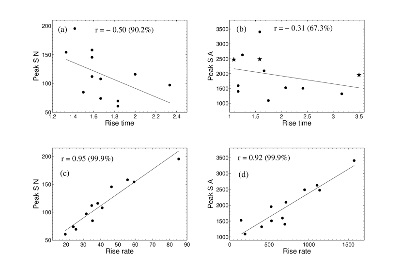
Figure 1: Observational evidences for WE1 (upper row) and WE2 (lower row). The upper row shows scatter diagrams plotting the peak values of (a) sunspot number and (b) sunspot area against rise times (in years). The data points of cycles 21, 22 and 23 are shown by stars in (b). The lower row shows scatter diagrams plotting the peak values of (c) sunspot number and (d) sunspot area against rise rates (in units of sunspot number per year). The straight lines are the best linear fits of the data. The linear correlation coefficients and the significance levels are also given on each plot.

If the rise time is taken as the time for a cycle to develop from a minimum to a maximum, then we have various difficulties. Usually we find an overlap between two successive cycles and the position of the minimum may get shifted depending on the amount of the overlap (Cameron & Schüssler 2007). Some cycles have plateau-like maxima with multiple peaks, so that it is difficult to say when the rising phase ended. If one of the later peaks is slightly higher than the earlier peak and one takes the later peak to indicate the end of the rise time, then one gets a “rise time” without any physical significance. This problem can be clearly seen in Fig. 1 of Dikpati, Gilman & de Toma (2008), where peaks in sunspot area for the cycles 21, 22 and 23 are seen to occur well after the cycles have reached the plateau-like tops. We see in the correlation plot given in Fig. 2 of Dikpati, Gilman & de Toma (2008) that these are some of the cycles which produced the maximum scatter and made the correlation disappear. To avoid the difficulties of ascertaining the minima and the maxima of the cycles, we define the rise time in the following way. Suppose a cycle has an amplitude $P$. We take the rise time to be the time during which the activity level changes from $0.2P$ to $0.8P$. The rise time defined in this way has a good anti-correlation with the cycle amplitude for all the data sets, the linear correlation coefficients and the significance levels for the four data types being: (1) $-0.50$ and $90.16\%$ for sunspot numbers; (2) $-0.42$ and $82.12\%$ for group sunspots; (3) $-0.31$ and $67.3\%$ for sunspot areas; and (4) $-0.33$ and $41\%$ for $10.7$ cm radio flux. The results for sunspot numbers and sunspot areas are shown in panels (a) and (b) of Fig. 1. It may be noted that the data points of cycles 21, 22 and 23 which were largely responsible for destroying the Waldmeier effect in the analysis of Dikpati, Gilman & de Toma (2008) are indicated by stars in Fig. 1(b) and are now quite close to the linear line. These results are very sensitive to the averaging bin size. If we average the data with a FWHM of $2$ yr instead of 1 yr, we obtain the following correlation coefficients and significance levels for the four data sets: (1) $-0.63$ and $97.28\%$; (2) $-0.60$ and $96.13\%$; (3) $-0.36$ and $75.38\%$; (4) $-0.67$ and $78.34\%$. If we calculate the rise time differently by taking the beginning and the end of the rise phase somewhat different from $0.2P$ and $0.8P$ (and also vary the FWHM while averaging the data), then we get somewhat but not significantly different correlation coefficients which are listed in Table 1 for sunspot area data.

Table 1: Linear correlation coefficients ($r$) and the significance levels ($s.l.$) between the rise time and the peak value of sunspot area data.

	FWHM = 1 yr	FWHM = 2 yr
Rise time	$r~{}(\%s.l.)$	$r~{}(\%s.l.)$
$0.2P$ to $0.8~{}P$	$-0.31~{}(67.3)$	$-0.36~{}(75.4)$
$0.2P$ to $0.7~{}P$	$-0.40~{}(79.9)$	$-0.42~{}(83.0)$
$0.2P$ to $0.65P$	$-0.43~{}(83.7)$	$-0.35~{}(74.2)$
$0.2P$ to $0.6~{}P$	$-0.47~{}(87.6)$	$-0.43~{}(83.7)$
$0.15P$ to $0.8~{}P$	$-0.32~{}(69.5)$	$-0.40~{}(79.8)$
$0.15P$ to $0.7~{}P$	$-0.43~{}(83.3)$	$-0.46~{}(86.7)$
$0.15P$ to $0.65P$	$-0.46~{}(86.7)$	$-0.40~{}(80.4)$
$0.15P$ to $0.6P$	$-0.50~{}(90.0)$	$-0.48~{}(88.2)$

We also study the second Waldmeier effect WE2 in all four data sets. We calculate the rise rate by determining the slope between two points at a separation of one year, with the first point one year after the sunspot minimum. We find strong correlation between the rates of rise and the amplitudes of the sunspot cycles. Results for sunspot number and sunspot area are shown in panels (c) and (d) of Fig. 1. Cameron & Schüssler (2008) have computed the rise rate slightly differently and obtained almost similar results.

We conclude that there is evidence for both WE1 and WE2 in different kinds of data sets.

2.2 Variations in meridional circulation

Only from mid-1990s we have reliable data on the variation of meridional circulation. Hathaway & Rightmire (2010) analyze these data to conclude that the meridional circulation varies with the sunspot cycle, becoming weaker at the time of the sunspot maximum. We should probably have to wait for at least one more full cycle to reach a firm conclusion whether this variation indeed has the same period as the sunspot cycle. A systematic variation of the meridional circulation having the same period as the sunspot cycle is not expected to introduce any irregularities in the theoretically computed sunspot cycles. Most of the dynamo calculations presented by our group (Chatterjee, Nandy & Choudhuri 2004; Choudhuri, Chatterjee, & Nandy 2004; Choudhuri, Chatterjee & Jiang 2007; Jiang, Chatterjee & Choudhuri 2007; Goel & Choudhuri 2009; Karak & Choudhuri 2009) assumed a constant meridional circulation because even a few years ago the available information about meridional circulation variation was very scanty.

Since a periodic variation of the meridional circulation with the sunspot cycle will not cause cycle irregularities, let us consider possible variations with longer time scales which may affect sunspot cycles. We have no direct information about variations of meridional circulation prior to 1995. However, if we believe that the solar dynamo is a flux transport dynamo and the period of a cycle is approximately inversely proportional to the meridional circulation during that cycle, then we can draw some conclusions about the variations in meridional circulation in the past from the periods of past sunspot cycles. At the outset, we point out that this is an unreliable and questionable procedure. Since we have no better way of inferring about variations in meridional circulation in the past, it is still worthwhile to see what conclusions we can draw from this procedure.

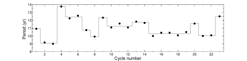
Figure 2: The points show the periods of last 23 solar cycles against cycle number. The solid line is indicative of the trend in variations of period as explained in the text.

Fig. 2 shows the periods of the various sunspot cycles beginning with cycle 1. If two successive cycles had similar periods, we may assume that the meridional circulation had similar strengths during these two cycles. We have put a solid line in Fig. 2 to indicate the trend of how periods of different cycles varied. Whenever successive cycles had periods varying less than 5% of the average period, we have made the solid line horizontal and indicative of the average period of those cycles. Only when periods of two successive cycles differed by more than 5%, there is a jump in the solid line in Fig. 2. If the solar dynamo is a flux transport dynamo in which the period is set by the amplitude of meridional circulation  then the solid line should give an idea how the meridional circulation varied in the past. It appears that during cycles 1–10, the meridional circulation had a relatively short coherence time, but probably not less than 15 yr. On the other hand, during cycles 11–20, the meridional circulation seemed to have a longer coherence time, but probably not longer than 45 yr. With the limited data we have, we cannot say whether the behaviour of cycles 1–10 is more typical in the long run or the behaviour of cycles 11–20 is more typical. Looking at Fig. 2, we can only surmise that the meridional circulation probably has long-time variations having coherence time lying somewhere between 15 yr and 45 yr. In §4 we shall present some simulations assuming the coherence time of the meridional circulation to be 30 yr. Since meridional circulation and differential rotation both arise from turbulent stresses in the convection zone, one intriguing and troubling question is whether variations of meridional circulation would be associated with the variations of differentia rotation. Since our theoretical understanding of this subject is still very primitive and also to focus our attention on how variations of meridional circulation affect the dynamo, we have taken differential rotation to be constant in our paper.

To summarize, even though it is difficult to draw firm conclusions, it seems that meridional circulation has fluctuations having coherence times somewhat longer than a cycle—probably of the order of 30 yr. It may be noted that Charbonneau & Dikpati (2000) argued that the meridional circulation would have fluctuations with coherence time of the order of a month, which is the eddy turnover time of solar convection. We do not find any observational signatures for such short-time fluctuations and such short-time fluctuations of the meridional circulation are not considered in this paper.

3 Mathematical Formulation

All our calculations are done with the code SURYA for solving the axisymmetric kinematic dynamo problem. An axisymmetric magnetic field can be represented in the form

$${\bf B}=B(r,\theta){\bf e}_{\phi}+\nabla\times[A(r,\theta){\bf e}_{\phi}],$$ (1)

where $B(r,\theta)$ and $A(r,\theta)$ respectively correspond to the toroidal and poloidal components. The standard equations for the kinematic dynamo are

$$\frac{\partial A}{\partial t}+\frac{1}{s}({\bf v}.\nabla)(sA)=\eta_{p}\left(\nabla^{2}-\frac{1}{s^{2}}\right)A+S(r,\theta,t)$$ (2)

$$\frac{\partial B}{\partial t}+\frac{1}{r}\left[\frac{\partial}{\partial r}(rv_{r}B)+\frac{\partial}{\partial\theta}(v_{\theta}B)\right]=\eta_{t}\left(\nabla^{2}-\frac{1}{s^{2}}\right)B$$

$$+s({\bf B}_{p}.\nabla)\Omega+\frac{1}{r}\frac{d\eta_{t}}{dr}\frac{\partial}{\partial{r}}(rB)$$ (3)

where $s=r\sin\theta$. Here ${\bf v}$ is the meridional circulation, $\Omega$ is the internal angular velocity of the Sun, $S(r,\theta,t)$ is the source term for the poloidal field by the Babcock–Leighton mechanism and $\eta_{p}$, $\eta_{t}$ are the turbulent diffusivities for the poloidal and toroidal components.

Since the internal rotation of the Sun has been determined by helioseismology, most of recent dynamo models use a profile of the angular velocity $\Omega$ consistent with helioseismic findings. Equation (8) of Chatterjee, Nandy & Choudhuri (2004) gives an analytical expression for $\Omega$ which is a good fit to helioseismology results. The profile of $\Omega$ obtained from this expression is shown in Fig. 1 of Chatterjee, Nandy & Choudhuri (2004). We use this $\Omega$ in all our calculations. While the angular velocity is now observationally constrained, different authors have modelled the meridional circulation, the poloidal source term and the turbulent diffusivities somewhat differently. This has given rise to varieties of solar dynamo models. In the last few years, however, two models have been studied fairly extensively—a high diffusivity model first developed by the group in Bangalore (Chatterjee, Nandy & Choudhuri 2004) and a low diffusivity model first developed by the group in Boulder (Dikpati & Charbonneau 1999). The turbulent diffusivities used in these models are shown respectively in Fig. 4 of Chatterjee, Nandy & Choudhuri (2004; solid line) and Fig. 1(D) of Dikpati & Charbonneau (1999). Both these models use a fairly low diffusivity in the tachocline (where turbulence is weak) to ensure that the advection of the toroidal field by meridional circulation dominates over diffusion there. However, the turbulent diffusion within the convection zone is assumed to be much larger. What Chatterjee, Nandy & Choudhuri (2004) call their ‘standard model’ was produced with a diffusivity of $2.4\times 10^{12}$ cm² s^-1 for the poloidal field within the convection zone, leading to a diffusion time of a few years across the convection zone. On the other hand, what Dikpati & Charbonneau (1999) call their ‘reference solution’ was produced with a much lower diffusivity of $5\times 10^{10}$ cm² s^-1, corresponding to a diffusion time of several centuries so that the magnetic fields are virtually frozen during the period of the dynamo. According to the classification scheme introduced by Yeates, Nandy & Mackay (2008), the model of Chatterjee, Nandy & Choudhuri (2004) is a ‘diffusion-dominated’ model, whereas the model of Dikpati & Charbonneau (1999) is an ‘advection-dominated’ model.

Jiang, Chatterjee & Choudhuri (2007; §5) gave several arguments that the diffusivity within the convection zone is likely to be fairly high as assumed by the group in Bangalore. Subsequently several other authors also have argued for high diffusivity (Goel & Choudhuri 2009; Choudhuri & Karak 2009; Hotta & Yokoyama 2010a, 2010b). It appears that such a high diffusivity is needed for getting the correct parity without an extra poloidal source term within the convection zone (Chatterjee, Nandy & Choudhuri 2004; Hotta & Yokoyama 2010b), for ensuring that the hemispheric asymmetry of magnetic activity remains small as observed (Chatterjee & Choudhuri 2006; Goel & Choudhuri 2009), for explaining the observed correlation of the polar field with the strength of the next cycle (Jiang, Chatterjee & Choudhuri 2007) and for keeping the polar field small in accordance with observational data (Hotta & Yokoyama 2010a). It may be noted that straightforward mixing length arguments also suggest a high diffusivity, Parker (1979, p. 629) concluding that the turbulent diffusivity within the convection zone should be of order $1$–$4\times 10^{12}$ cm² s^-1. We carry out our calculations with the high diffusivity model and show that the theoretical model predicts the Waldmeier effect roughly in accordance with the observational data. For the sake of completeness, we also explore the low diffusivity Dikpati-Charbonneau (1999) model and find that this model is unable to explain WE1.

Table 2: The original values of the parameters in the standard model (§4 of Chatterjee, Nandy & Choudhuri 2004) along with the changed values we use here are given.

Parameter	Standard Model	This Model
$\eta_{SCZ}$	$2.4\times 10^{12}$ cm2 s-1	$3.0\times 10^{12}$ cm2 s-1
$v_{0}$	$-29$ m s-1	$-23$ m s-1
$R_{p}$	$0.61R_{\odot}$	$0.635R_{\odot}$
$\alpha_{0}$	25 m s-1	30 m s-1
$\beta_{2}$	$1.8\times 10^{-8}$ m-1	$1.3\times 10^{-8}$ m-1
$\Gamma$	$3.47\times 10^{8}$ m	$3.0253\times 10^{8}$ m
$r_{0}$	$0.1125R_{\odot}$	$0.1286R_{\odot}$
$d_{tac}$	$0.025R_{\odot}$	$0.03R_{\odot}$

The ‘standard model’ of Chatterjee, Nandy & Choudhuri (2004) produced a period somewhat larger than 11 yr. Also the value of the meridional circulation near the surface was somewhat larger than what is observed. For the calculations presented in this paper, we have changed some parameters of the ‘standard model’ to make the period 11 yr and to make the meridional circulation at the surface equal to 23 m s^-1. Table 2 lists the values of those parameters which have their values changed in this paper from the values used by Chatterjee, Nandy & Choudhuri (2004). Except the values of these parameters listed in Table 2, our model remains the same as the ‘standard model’ of Chatterjee, Nandy & Choudhuri (2004). We make a few comments on some aspects of this model. The meridional circulation in the northern hemisphere is obtained from Equations (9)–(11) of Chatterjee, Nandy & Choudhuri (2004), from which we get the meridional circulation in the southern hemisphere by antisymmetry. Although we now choose some parameters of the meridional circulation slightly differently from Chatterjee, Nandy & Choudhuri (2004) as listed in Table 2, the streamlines of meridional circulation still look almost the same as in Fig. 2 of Chatterjee, Nandy & Choudhuri (2004). The meridional circulation used by us penetrates slightly below the bottom of the convection zone, which is essential for confining the butterfly diagram to lower latitudes (Nandy & Choudhuri 2002). It may be noted that there is a controversy at the present time whether the meridional circulation can penetrate below the convection zone—arguments having been advanced both against it (Gilman & Miesch 2004) and for it (Garaud & Brummel 2008). Recently Chakraborty, Choudhuri & Chatterjee (2009) have argued that the early initiation of torsional oscillations at latitudes higher than the typical sunspot latitudes is possible only with such a penetrating meridional circulation, providing another strong support for it. The diffusion coefficients $\eta_{p}$ and $\eta_{t}$ are shown in Fig. 4 of Chatterjee, Nandy & Choudhuri (2004), where the justification for using two different diffusivities is discussed. Basically diffusion of the toroidal field is suppressed inside concentrated flux tubes. Since these flux tubes are not resolved in the mean field theory, we capture this effect approximately by making $\eta_{t}$ smaller than $\eta_{p}$ in the mean field equations.

For checking whether a low diffusivity model can explain the Waldmeier effect, we have used the model of Dikpati & Charbonneau (1999). It may be noted that this model, which produces butterfly diagrams extending to high latitudes, was subsequently modified by Dikpati et al. (2004) to build what they call a ‘calibrated flux transport dynamo’. It is this ‘calibrated flux transport dynamo’ model which was used by Dikpati & Gilman (2006) to predict that the cycle 24 will be very strong. However, this ‘calibrated flux transport dynamo’ of Dikpati et al. (2004) has so far not been reproduced by any independent code of any other group. Some of the other groups who tried to reproduce this model were unable to do so (Jiang, Chatterjee & Choudhuri 2007; Hotta & Yokoyama 2010a). We also have tried to reproduce the results of Dikpati et al. (2004) and could not, although we are able to reproduce the results of Dikpati & Charbonneau (1999). Jiang, Chatterjee & Choudhuri (2007) noted that the ‘reference solution’ of Dikpati & Charbonneau (1999) was reproduced when the amplitude of meridional circulation was taken $u_{0}=20$ m s^-1 rather than $u_{0}=10$ m s^-1 as reported by Dikpati & Charbonneau (1999). We also confirm this. We have, however, taken the value $u_{0}=$ 14.5 m s^-1 to ensure that the dynamo period comes out to be 11 yr. Everything else in the low diffusivity model we use in this paper remains the same as in the ‘reference solution’ of Dikpati & Charbonneau (1999).

To study whether the theoretical models can explain the Waldmeier effect, we have to introduce irregularities in the theoretical model to make the cycles unequal. In the next section, we describe how we introduce fluctuations in the poloidal field source term and in the meridional circulation, and we present the results we get by introducing these fluctuations. To look for the Waldmeier effect, we need to find out how the sunspot number varies with time. Charbonneau & Dikpati (2000) proposed that the magnetic energy density at latitude 15^∘ at the base of the convection zone ($r=0.7R_{\odot}$) can be taken to be a good proxy of the sunspot number and used this to produce the sunspot number plots which they presented. We also take this as a proxy for the sunspot number in this paper for both the high diffusivity and low diffusivity models.

4 Results from theoretical models

We now present the results obtained by using both the high diffusivity (or diffusion-dominated) model and the low diffusivity (or advection-dominated) model introduced in §3. After introducing irregularities in the models, we generate the sunspot number plot for a particular run by using the magnetic energy density at latitude 15^∘ at the base of the convection zone as the proxy of the sunspot number. Then the rise time and the rise rate are calculated exactly the way they were done for the observational data as described in §2.1. We shall first present the results obtained by introducing fluctuations in the poloidal field generation and then present results with fluctuations in the meridional circulation. It may be noted that Charbonneau & Dikpati (2000) presented some results by introducing these two kinds of fluctuations in their low diffusivity model. However, we introduce the fluctuations somewhat differently and, in one important case, we find a result which is opposite of what Charbonneau & Dikpati (2000) presented, as we shall point out.

4.1 Fluctuations in the poloidal field generation

As argued by Choudhuri, Chatterjee & Jiang (2007) and Jiang, Chatterjee & Choudhuri (2007), the cumulative effect of fluctuations in the Babcock–Leighton process which produces the poloidal field can be incorporated by stopping the dynamo code at every minimum and then multiplying the poloidal field above $0.8R_{\odot}$ by a factor $\gamma$. We now present results of runs for both the high and low diffusivity models in which $\gamma$ at a minimum was taken to be a random number lying in the range 0.5–1.5.

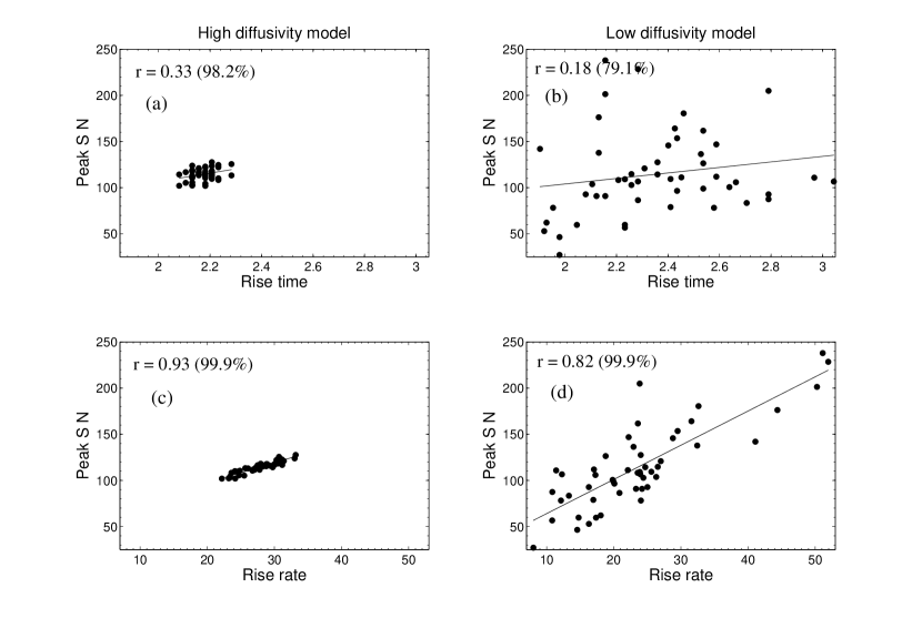
Figure 3: Theoretical plots of WE1 (upper row) and WE2 (lower row) obtained by introducing fluctuations in the poloidal field at the minima. The upper figures (a) and (b) show the scatter diagrams between the rise time (in years) and the peak sunspot number, whereas the lower figures (c) and (d) show the scatter diagrams between the rise rate (in units of sunspot number per year) and the peak sunspot number. The left figures (a) and (c) are from the high diffusivity model, whereas the right figures (b) and (d) are from the low diffusivity model. The straight lines are the best linear fits of the data. The correlation coefficients and the significance levels are also given on each plot.

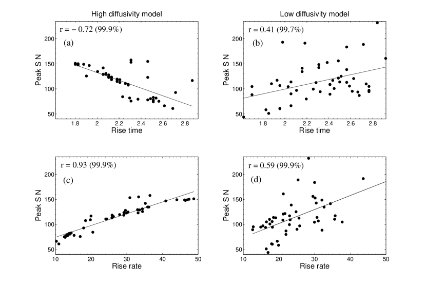
Figure 4: Theoretical plots obtained by introducing fluctuations in the meridional circulation. The four figures correspond to the same things as in Fig. 3.

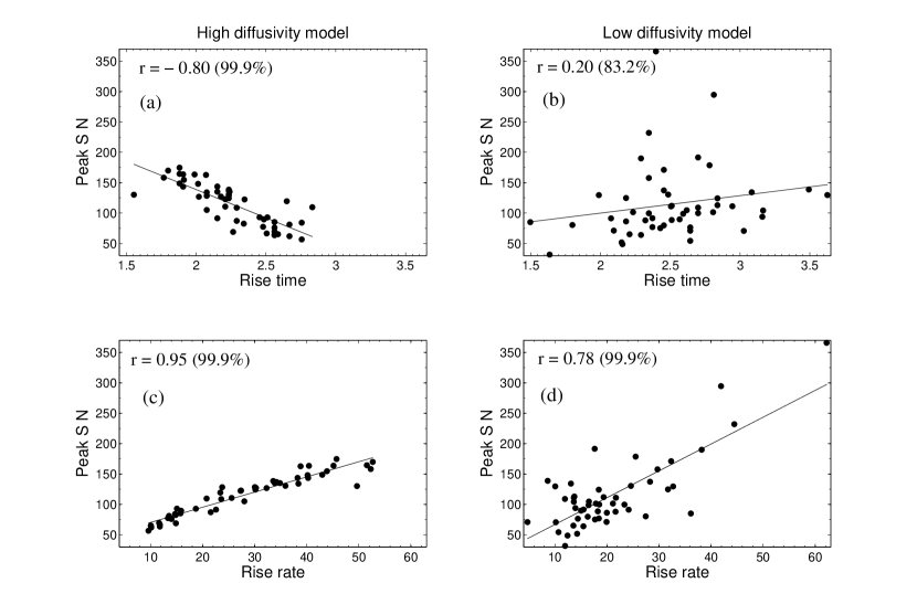
Figure 5: Theoretical plots obtained by introducing fluctuations in both the poloidal field generation and the meridional circulation. The four figures correspond to the same things as in Fig. 3.

First, let us look at the lower panels of Fig. 3 which show the correlations between the rise rate and the peak sunspot number in the high and low diffusivity cases respectively. In both the cases, it is found that cycles with stronger peaks tend to have higher rise rates, in accordance with the observed WE2. It is easy to understand why this is so. As long as the meridional circulation is held constant, the periods of various cycles in a flux transport dynamo do not vary too much. However, fluctuations in the poloidal field generation make the strengths of different cycles unequal. A strong cycle has to rise to a higher value of peak sunspot number compared to a weak cycle in approximately the same amount of time. Therefore, a stronger cycle has to have a higher rise rate. This is true irrespective of whether the diffusivity is high or low. We thus conclude that fluctuations in poloidal field generation can easily account for the effect WE2.

Although we believe that the effect WE1 involving the rise time is primarily produced by fluctuations in the meridional circulation, the upper panels in Fig. 3 show the correlations between the rise time and the peak sunspot number when fluctuations in the poloidal field generation alone are present. For both the high and low diffusivity cases, the theoretical results (a positive correlation) are the opposite of the observational effect WE1 (anti-correlation). In the high diffusivity model, the fluctuations in the poloidal field generation do not cause much variations in the cycle periods and the variations in rise time are seen to be rather small in Fig. 3a. On the other hand, we see in Fig. 3b that rise times have a much larger spread for the low diffusivity model. Presumably fluctuations in the high diffusivity model are damped out within a few years and cannot cause so much variations in the durations of cycles. On the other hand, fluctuations in the low diffusivity model persist for times much longer than the period of the dynamo and can affect the durations of cycles. In both cases, however, fluctuations in poloidal field generation alone cannot account for WE1. We need something else—presumably fluctuations in the meridional circulation.

It may be noted that Charbonneau & Dikpati (2000) reported a weak anti-correlation between cycle duration and cycle amplitude on introducing fluctuations in the poloidal source term (see their Fig. 6C). It is true that Charbonneau & Dikpati (2000) treated the fluctuations in the poloidal source term somewhat differently from what we are doing and plotted the cycle amplitude against the cycle duration rather than the rise time. However, we repeated their procedure for the low diffusivity model and found that we still get a weak correlation similar to our Fig. 3b rather than the weak anti-correlation seen in their Fig. 6C. It should be noted that, when runs are repeated with different realizations of random numbers, the correlation coefficients turn out to be somewhat different. It is true that we and Charbonneau & Dikpati (2000) got rather small correlation coefficients of opposite sign: $r=0.18$ and $r=-0.23$ respectively. To some extent, these differences may be due to statistical uncertainties in different numerical realizations of the same problem involving fluctuations created by random numbers. However, in the several runs we performed, we never got a negative correlation coefficient. It will be worthwhile for other groups to check this independently.

The fact that fluctuations in the poloidal field generation do not introduce much variations in cycle durations in the diffusion-dominated model but introduce more variations in the advection-dominated model has another significance. The arguments we have given in §2.2 about variations in meridional circulation are based on the assumption that periods of cycles do not vary much as long as the meridional circulation is held constant. As we now see, this is strictly true only for the diffusion-dominated dynamo. As we believe the solar dynamo to be diffusion-dominated, the arguments we have given in §2.2 should be valid for the meridional circulation in the Sun.

4.2 Fluctuations in the meridional circulation

We now study the results of introducing fluctuations in the meridional circulation. As we argued in §2.2, fluctuations in the meridional circulation seem to have a coherence time of about 30 years if we believe that the periods of past cycles were indicative of the variations in meridional circulation. We run our code by changing the amplitude of the meridional circulation abruptly after every 30 years. It appears that the high diffusivity (or diffusion-dominated) model requires a stronger fluctuation in the meridional circulation compared to the low diffusivity (or advection-dominated) model to introduce the same kinds of variations in cycle periods. We use a 30% amplitude fluctuation in the high diffusivity model and a 20% amplitude fluctuation in the low diffusivity model.

The results are shown in Fig. 4. For both the models, the rise rate is correlated with the peak sunspot number, as seen in the lower panels of Fig. 4. In other words, the effect WE2 is reproduced from the theoretical models easily whether the diffusivity is high or low. However, we see a dramatic difference between the two models when we look at the plots of peak sunspot number against rise time (the two upper panels in Fig. 4). For the high diffusivity model, we find that the rise time is anti-correlated with the peak sunspot number, in accordance with the Waldmeier effect WE1. On the other hand, the low diffusivity model shows a correlation, which is the opposite of the observed Waldmeier effect WE1. We point out that Charbonneau & Dikpati (2000) also reported such a positive correlation (opposite of the Waldmeier effect) on introducing fluctuations in the meridional circulation in their low diffusivity model (see their Fig. 4C), although they introduced the fluctuations differently from what we are doing.

To understand the physics behind this dramatic difference between the two models, the readers are advised to refer to Fig. 5 of Yeates, Nandy & Mackay (2008) and the associated discussion. Let us summarize the main argument. Suppose the meridional circulation has become weaker during a cycle. Then the duration of the cycle will be longer and the magnetic fields will spend more time at the bottom of the convection zone. This will result in two opposing effects. Diffusion will have more time to act on the magnetic fields, trying to make the cycle weaker. On the other hand, differential rotation will have more time to act on the poloidal field, building up a larger toroidal field and making the cycle stronger. Whether the cycle will be weaker or stronger will depend on which of these two effects win over. In the high diffusivity (or diffusion-dominated) model, diffusivity acting on the magnetic fields is the more important effect. Hence, when the meridional circulation is weaker, the cycle duration (as well as the rise time) is more and the strength of the cycle is lower, leading to the anti-correlation in accordance with the Waldmeier effect, as seen in Fig. 4a. The opposite of this happens in the low diffusivity (or advection-dominated) model, where the differential rotation building up a stronger toroidal field is the more important effect. A weaker meridional circulation causing a longer rise time will be associated with a stronger cycle, opposite of the Waldmeier effect WE1, as seen in Fig. 4b.

We thus see that the high and low diffusivity models give very different results when fluctuations in the meridional circulation are introduced. Only the high diffusivity model can explain the Waldmeier effect WE1, while the low diffusivity model gives the opposite result. The effect WE2 is, however, explained by both the models.

4.3 Effect of combined fluctuations

Finally we present results for cases where fluctuations in both the poloidal field generation and the meridional circulation are present. As we already mentioned, we have introduced fluctuations in the poloidal field generation in §4.1 in a way somewhat different from what Charbonneau & Dikpati (2000) had done. In the calculations presented in §4.1, we have introduced the cumulative effect of poloidal source fluctuations by multiplying the poloidal field above $0.8R_{\odot}$ by a number $\gamma$ at each minimum. We have also done some calculations by introducing fluctuations in the poloidal source term by the methodology of Charbonneau & Dikpati (2000), in which the amplitude of $\alpha$ is changed randomly after a coherence time of 1 month, the level of fluctuations in the amplitude of $\alpha$ being another parameter in the problem. The results obtained by the two methodologies are found to be very similar. Here we now present results in which fluctuations in meridional circulation are introduced exactly as what we had done in §4.2, but fluctuations in poloidal field source are introduced by the methodology of Charbonneau & Dikpati (2000) which involves a fluctuation in the $\alpha$-effect (Choudhuri 1992). Both for the high and low diffusivity models, the amplitude of $\alpha$ is changed after the coherence time 1 month, the level of fluctuations being 100% for the high diffusivity model and 200% for the low diffusivity model. Charbonneau & Dikpati (2000) had also used 200% fluctuations in their low diffusivity model.

The results are shown in Fig. 5. Since both kinds of fluctuations taken individually produced a direct correlation between rise rate and peak sunspot number in both the high and low diffusivity models (the lower panels in Figs. 3 and 4), we naturally expect such a correlation to arise when both kinds of fluctuations are combined. This is clearly seen in the lower panels of Fig. 5, indicating that WE2 is a robust result and can be produced in theoretical models irrespective of whether the diffusivity is high or low. However, when we look for the Waldmeier effect WE1 in the correlation between rise time and peak sunspot number, then the situation is more complicated. For the low diffusivity model, both kinds of fluctuations taken individually produced a direct correlation between them, which is the opposite of the Waldmeier effect (Figs. 3b and 4b). Not surprisingly, we see a direct correlation when the two kinds of fluctuations are combined. We thus conclude that the low diffusivity model cannot explain the Waldmeier effect WE1. For the high diffusivity model, we had a direct correlation when fluctuations in poloidal field generation alone were present (Fig. 3a) and an anti-correlation when fluctuations in meridional circulation alone were present (Fig. 4a), the spread in rise times being rather small in Fig. 3a. When both these kinds of fluctuations are combined, we find an anti-correlation as seen in Fig. 5a. Thus the high diffusivity model reproduces the Waldmeier effect WE1. To sum up, the Waldmeier effect WE1 is reproduced theoretically only in the high diffusivity model and not in the low diffusivity model when fluctuations in both the poloidal field generation and meridional circulation are included.

It may be noted that, even in the high diffusivity model, we need to make the coherence time of meridional circulation fluctuations somewhat longer than the cycle period (we have taken 30 yr for the results presented in Figs. 4–5) in order to obtain the Waldmeier effect WE1. If the coherence time is made comparable to the cycle period (10 or 15 yr), then we do not get WE1. For a coherence time of 20 yr for meridional circulation fluctuations, we still find the Waldmeier effect WE1 with the correlation coefficient and the significance level equal to $-0.43$ and $99.8\%$ respectively for a particular run instead of $-0.80$ and $99.9\%$ indicated in Fig. 5a.

5 Conclusion

To the best of our knowledge, this is the first systematic effort of addressing the question whether the Waldmeier effect can be explained on the basis of flux transport dynamo models of the sunspot cycle. Along with the Waldmeier effect that rise times of cycles are anti-correlated with cycle amplitudes, which we call WE1, we also consider the related effect that rise rates are correlated with cycle amplitudes, which we call WE2. In view of a recent controversy whether the Waldmeier effect exists in different kinds of data, we point out that, if we define rise times and rise rates carefully, then we find evidence for both WE1 and WE2 in different kinds of data.

We can think of two main sources of irregularities in the dynamo cycles: fluctuations in the Babcock–Leighton mechanism and fluctuations in the meridional circulation. We study the effects of both kinds of fluctuations on the dynamo models. Since not much is known about long-term fluctuations of the meridional circulation, we analyze the periods of the past sunspot cycles in §2.2 to draw some tentative conclusions about fluctuations of the meridional circulation in the past.

The main conclusion of our paper is that the effects of fluctuations are dramatically different in high and low diffusivity models. This is not surprising. Fluctuations in the high diffusivity model damp out in a few years. On the other hand, fluctuations in the low diffusivity model take times longer than the dynamo cycle to damp out. The left panels in Figs. 3, 4 and 5 show results obtained with the high diffusivity model, whereas the right panels show results for the low diffusivity model. Even a cursory look at these figures shows that similar fluctuations produce much larger dispersions in the low diffusivity model. As long as the meridional circulation is held constant, durations of cycles do not vary much in the high diffusivity model even after introducing fluctuations in the poloidal field generation process. This is seen in Fig. 3a. But this is not so true in the low diffusivity model, as can be seen in Fig. 3b.

We find that the effect WE2 is very robust and is reproduced easily in different types of dynamo models subjected to different types of fluctuations, as seen in the bottom panels of Figs. 3, 4 and 5. Basically, a stronger cycle rises to its higher peak at a faster rate. The most important result of our paper is that the Waldmeier effect WE1 arises from the fluctuations in the meridional circulation and this happens only for the high diffusivity model. The low diffusivity model gives the opposite result. We pointed out how we can understand this physically on the basis of the analysis presented by Yeates, Nandy & Mackay (2008). In the high diffusivity (or diffusion-dominated) model, the longer cycle allows the diffusivity to act for a longer time and results in the cycle being weaker, in accordance with the Waldmeier effect. In the low diffusivity (or advection-dominated) model, on the other hand, a longer cycle means that the differential rotation builds up the toroidal field to a stronger value, thus giving the opposite of the Waldmeier effect. Jiang, Chatterjee & Choudhuri (2007, §5) gave several arguments why the turbulent diffusivity inside the convection zone has to be sufficiently high to ensure that the diffusion time is not more than a few years. Several subsequent authors reinforced this point (Goel & Choudhuri 2009; Choudhuri & Karak 2009; Hotta & Yokoyama 2010a, 2010b). The fact that only the high diffusivity model can explain the Waldmeier effect makes the case still stronger that the solar dynamo is a high diffusivity or diffusion-dominated dynamo.

We finally come to the last question whether the high diffusivity model reproduces the observational data not only qualitatively, but also quantitatively. The unit of the sunspot number in the theoretical plots is chosen in such a way that the sunspot number of an average cycle comes out to be $114.5$ (which is the average value of the peak sunspot numbers of last $12$ cycles). With this choice of unit for the vertical axes in Figs. 3, 4 and 5, the theoretical plots can be readily compared with the observational plots. Perhaps Fig. 5 with both kinds of fluctuations present is the appropriate figure to compare with observations. We should compare Fig. 1a with Fig. 5a and Fig. 1c with Fig. 5c. Although the theoretical plots have more data points than the observational plots, a comparison of the values on the horizontal and vertical axes shows that the spreads in rise rate, rise time and peak sunspot number are comparable in the observational and theoretical plots. It is true that the observational plots seem to have a little bit more scatter compared to the theoretical plots, which is particularly evident when we compare Fig. 1a with Fig. 5a. In spite of this, most readers will hopefully agree with us that the comparisons between theory and observations seem reasonably satisfactory, suggesting that the characteristics of the fluctuations we had assumed in our theoretical analysis probably are not very far from reality. It should be kept in mind that such calculations involving random numbers give slightly different results for different runs. The run which produced Fig. 5 was repeated several times to ensure that the results for the different runs were only slightly different.

Acknowledgments: We thank an anonymous referee for valuable comments, which helped in improving the paper. This work is partly supported by DST, India (project No.SR/S2/HEP–15/2007). BBK thanks CSIR, India for financial support.

References

- Babcock (1961) Babcock H. W., 1961, ApJ, 133, 572
- Chakraborty, Choudhuri & Chatterjee (2009) Chakraborty S., Choudhuri A. R., Chatterjee P., 2009, Phys. Rev. Lett., 102, 041102
- Cameron & Schussler (2008) Cameron R., Schussler M., 2008, ApJ, 659, 801
- Cameron & Schussler (2007) Cameron R., Schussler M., 2007, ApJ, 685, 1291
- Charbonneau & Dikpati (2000) Charbonneau P., Dikpati M., 2000, ApJ, 543, 1027
- Chatterjee & Choudhuri (2006) Chatterjee P., Choudhuri A. R., 2006, Sol. Phys., 239, 29
- Chatterjee, Nandy & Choudhuri (2004) Chatterjee P., Nandy D., Choudhuri A. R., 2004, A&A, 427, 1019
- Choudhuri (1989) Choudhuri A. R. 1989, Sol. Phys., 123, 217
- Choudhuri (1992) Choudhuri A. R. 1992, A&A, 253, 277
- Choudhuri (1998) Choudhuri A. R., 1998, The Physics of Fluids and Plasmas: An Introduction for Astrophysicists. Cambridge Univ. Press, Cambridge
- Choudhuri (2003) Choudhuri A. R. 2003, Sol. Phys., 215, 31
- Choudhuri, Chatterjee & Jiang (2007) Choudhuri A. R., Chatterjee P., Jiang J., 2007, Phys. Rev. Lett., 98, 1103
- Choudhuri, Chatterjee & Nandy (2004) Choudhuri A. R., Chatterjee P., Nandy D., 2004, ApJ, 615, L57
- Choudhuri & Karak (2009) Choudhuri A. R., Karak B. B., 2009, RAA, 9, 953
- Choudhuri, Schüssler & Dikpati (1995) Choudhuri A. R., Schüssler M., Dikpati M., 1995, A&A, 303, L29
- Dikpati & Charbonneau (1999) Dikpati M., Charbonneau P., 1999, ApJ, 518, 508
- Dikpati et al. (2004) Dikpati M., de Toma G., Gilman P. A., Arge C. N., White O. R., 2004, ApJ, 601, 1136
- Dikpati & Gilman (2006) Dikpati M., Gilman P. A., 2006, ApJ, 649, 498
- Dikpati, Gilman & de Toma (2008) Dikpati M., Gilman P. A., de Toma, G., 2008, ApJ, 673, L99
- D’Silva & Choudhuri (1993) D’Silva S., Choudhuri A. R., 1993, A&A, 272, 621
- Durney (1995) Durney B. R., 1995, Sol. Phys., 160, 213
- Garaud & Brummel (2008) Garaud P., Brummel N. H., 2008, ApJ, 674, 498
- Gilman & Miesch (2004) Gilman P. A., Miesch M. S., 2004, ApJ, 611, 568
- Goel & Choudhuri (2009) Goel A., Choudhuri A. R., 2009, RAA, 9, 115
- Hathaway & Rightmire (2010) Hathaway D. H., Rightmire L., 2010, Sci., 327, 1350
- Hathaway, Wilson & Reichmann (2002) Hathaway D. H., Wilson R. M., Reichmann E. J., 2002, Sol. Phys., 211, 357
- (27) Hotta H., Yokoyama T., 2010a, ApJ, 709, 1009
- (28) Hotta H., Yokoyama T., 2010b, ApJ, 714, L308