Stellar dynamos in the transition regime: multiple dynamo modes and anti-solar differential rotation

Abstract

Global and semi-global convective dynamo simulations of solar-like stars are known to show a transition from an anti-solar (fast poles, slow equator) to solar-like (fast equator, slow poles) differential rotation (DR) for increasing rotation rate. The dynamo solutions in the latter regime can exhibit regular cyclic modes, whereas in the former one, only stationary or temporally irregular solutions have been obtained so far. In this paper we present a semi-global dynamo simulation in the transition region, exhibiting two coexisting dynamo modes, a cyclic and a stationary one, both being dynamically significant. We seek to understand how such a dynamo is driven by analyzing the large-scale flow properties (DR and meridional circulation) together with the turbulent transport coefficients obtained with the test-field method. Neither an $\alpha\Omega$ dynamo wave nor an advection-dominated dynamo are able to explain the cycle period and the propagation direction of the mean magnetic field. Furthermore, we find that the $\alpha$ effect is comparable or even larger than the $\Omega$ effect in generating the toroidal magnetic field, and therefore, the dynamo seems to be $\alpha^{2}\Omega$ or $\alpha^{2}$ type. We further find that the effective large-scale flows are significantly altered by turbulent pumping.

1 Introduction

Recently, Brandenburg & Giampapa (2018) reported on an abrupt increase of the magnetic activity level of solar-like stars with decreasing values of the Coriolis number in the vicinity of its solar value, with the Coriolis number quantifying the rotational influence on convection. Another observational study (Olspert et al., 2018) found that the degree of magnetic variability abruptly decreased, indicative of the disappearance of magnetic cycles, at slightly lower than solar chromospheric activity index values. Moreover, Metcalfe et al. (2016) interpreted Kepler data to indicate that the Sun is rotationally and magnetically in a transitional state, where the global magnetic dynamo is shutting down. Brandenburg & Giampapa (2018) proposed a transition in the differential rotation (DR) from solar-like (for younger stars) to anti-solar (at a later age) to be responsible for some of these phenomena.

This transition (henceforth AS-S transition) has already been the subject of many numerical studies (see, e.g., Gastine et al., 2014; Käpylä et al., 2014; Mabuchi et al., 2015; Featherstone & Miesch, 2015; Viviani et al., 2018) and they all pinpoint it in a narrow Coriolis number interval around its solar value. The latter can be estimated, for example, from mixing-length models to be around two (e.g. Käpylä et al., 2014). However, none of these works considered dynamo solutions near the transition point. They either studied the cyclic modes in the solar-like rotation regime, or the stationary and temporally irregular ones (Karak et al., 2015; Warnecke, 2018) obtained in the anti-solar regime.

In a previous paper (Viviani et al., 2018), we reported on dynamo simulations of solar-like stars with varying rotation rate, two of which showed oscillatory behavior in the AS-S transition. In these simulations, the poleward migration of the magnetic field is accompanied by a rotation profile exhibiting a decelerated equator and faster polar regions (anti-solar DR). The aim of the present paper is to study how such transitional–regime dynamos operate.

In the regime of solar-like DR, cyclic dynamo solutions with equatorward dynamo waves are often obtained from global magneto-convection models (e.g. Käpylä et al., 2012; Augustson et al., 2015; Strugarek et al., 2017). Most of them can be explained in terms of Parker waves (see, e.g., Warnecke et al., 2014, 2016, 2018; Käpylä et al., 2016, 2017; Warnecke, 2018). The migration direction and cycle period of such waves is determined by the product of the $\alpha$ effect and the radial gradient of the local rotation rate $\Omega$ (Parker, 1955; Yoshimura, 1975). For an equatorward-migrating field in the northern hemisphere (as observed on the Sun), one needs, for example, a negative radial gradient of $\Omega$ and a positive $\alpha$ effect. However, simplified dynamo models often invoke an advection-dominated concept (e.g. Choudhuri et al., 1995; Dikpati & Charbonneau, 1999; Küker et al., 2001) to explain the migration and cyclic behavior of large-scale stellar magnetic fields. In this case, the meridional flow speed and direction at the location of the toroidal field generation determine the cycle period and latitudinal dynamo wave direction.

Another possible mechanism generating cyclic dynamo solutions is an $\alpha^{2}$ dynamo (Baryshnikova & Shukurov, 1987; Rädler & Bräuer, 1987; Brandenburg, 2017). In this case, magnetic field generation is due to the $\alpha$ effect alone, and DR is not needed. Such a dynamo was reproduced in forced turbulence in a spherical shell (Mitra et al., 2010) and convection simulations in a box (Masada & Sano, 2014), but global convective dynamo models have not yet yielded a similar solution.

In this work, we will investigate the properties of one particular transitional–regime dynamo solution, and test which mechanisms can explain the seen cyclic behavior. To achieve this goal we will use the test-field method (Schrinner et al., 2005, 2007) for extracting the turbulent transport coefficients. This is possible due to the dominance of the axisymmetric magnetic field allowing us to try a description in terms of mean-field theory. The test-field method has been successfully used in previous studies to explain planetary dynamos (e.g. Schrinner, 2011; Schrinner et al., 2011, 2012), cyclic dynamo solutions of solar-type stars (Warnecke et al., 2018; Warnecke, 2018), and the long-term variations of these solutions (Gent et al., 2017).

2 Setup and Methods

We use the Pencil Code to solve the fully compressible magnetohydrodynamic equations for the velocity ${\boldsymbol{U}}$, the density $\rho$, the specific entropy $s$ and the magnetic vector potential ${\boldsymbol{A}}$ with the magnetic field ${\boldsymbol{B}}=\mbox{\boldmath$\nabla$}{}\times{\boldsymbol{A}}$ in a spherical shell without polar cap, defined in spherical coordinates $(r,\theta,\phi)$ by $0.7R\leq r\leq R$ for the radial extent, with $\theta_{0}\leq\theta\leq\pi-\theta_{0}$ and $0\leq\phi\leq 2\pi$ for the extents in colatitude and longitude, respectively, where $\theta_{0}=15^{\circ}$. The setup is the same as the one used in Käpylä et al. (2013) and Viviani et al. (2018). We impose impenetrable and stress-free boundary conditions at all radial and latitudinal boundaries for the velocity field ${\boldsymbol{U}}$, and a perfect-conductor boundary condition at the bottom and the latitudinal boundaries for ${\boldsymbol{B}}$, while at the top, the field is forced to be radial. The temperature follows a blackbody condition at the top, whereas a constant heat flux is prescribed at the bottom. At the latitudinal boundaries, zero heat flux is enforced. We start with an isentropic atmosphere for density and entropy, see Käpylä et al. (2013) for details. The initial conditions for the magnetic field and the velocity are weak Gaussian seeds.

Nondimensional input parameters for the examined run are the Taylor number, or correspondingly the Ekman number, defined as

$${\rm Ta}=\left(2\Omega_{0}\left(\Delta r\right)^{2}/\nu\right)^{2}={\rm Ek}^{-2}=2.03\cdot 10^{7},$$ (1)

where $\Omega_{0}$ is the overall rotation rate with $\Omega_{0}/\Omega_{\sun}=1.8$ for the considered run, $\Delta r=0.3R$ is the thickness of the shell, and $\nu$ is the constant viscosity. Further, we have the thermal, sub-grid scale (SGS) thermal and magnetic Prandtl numbers, the latter two describing the unresolved turbulent effects:

$${\rm Pr}\!=\!\frac{\nu}{\chi^{\rm m}}=58,\ {\rm Pr}_{\rm SGS}\!=\!\frac{\nu}{\chi^{\rm m}_{\rm SGS}}=2.5,\ {\rm Pr}_{\rm M}\!=\!\frac{\nu}{\eta}=1,$$ (2)

Here, $\chi^{\rm m}$ is the heat diffusivity calculated in the middle of the convective zone at $r^{\rm m}=0.85R$ as $\chi^{\rm m}=K\left(r^{\rm m}\right)/c_{P}\rho\left(r^{\rm m}\right)$, $c_{P}$ being the specific heat at constant pressure. The radiative heat conductivity $K$ follows an $r^{-15}$ dependency to mimic the actual heat flux profile in the Sun. $\chi_{\rm SGS}^{\rm m}$ is the turbulent heat diffusivity at $r=r^{\rm m}$ (see Käpylä et al., 2013, for details) and $\eta$ is the constant magnetic diffusivity.

The non-dimensional quantities are scaled to physical units using the solar radius $R=7\cdot 10^{8}~{}{\rm m}$, solar rotation rate $\Omega_{\sun}=2.7\cdot 10^{-6}~{}{\rm s^{-1}}$, the density at the bottom of the solar convection zone $\rho(0.7R)=\rho_{0}=200~{}{\rm kgm^{-3}}$, and $\mu_{0}=4\pi\cdot 10^{-7}~{}{\rm Hm^{-1}}$. The initial density contrast in the simulation is roughly 30, and the dimensionless luminosity $\mathcal{L}=L_{0}/[\rho_{0}(GM)^{3/2}R^{1/2}]\approx 3.8\cdot 10^{-5}$, where $L_{0}$ is the luminosity in the simulation, $G$ is the gravitational constant and $M$ the mass of the star. This corresponds to an approximately $10^{6}$ times higher luminosity than the solar one, $L_{\odot}$, to avoid the acoustic timestep constraint. The rotation rate is increased correspondingly in proportion to $\left(L_{0}/L_{\odot}\right)^{1/3}$, to obtain a realistic rotational influence on the flow (for further details see Appendix A of Käpylä et al., 2019).

We indicate by $\overline{\boldsymbol{B}}$ and $\overline{\boldsymbol{U}}$ the mean (longitudinally averaged) fields, and by ${\boldsymbol{b}}^{\prime}$, ${\boldsymbol{u}}^{\prime}$ the corresponding fluctuating fields, so that, for example, ${{\boldsymbol{B}}}=\overline{\boldsymbol{B}}+{\boldsymbol{b}}^{\prime}$.

The need to compute turbulent transport coefficients can be seen from the induction equation for the mean magnetic field, $\overline{\boldsymbol{B}}$:

$$\frac{\partial\overline{\boldsymbol{B}}}{\partial t}=\mbox{\boldmath$\nabla$}{}\times\left(\overline{\boldsymbol{U}}\times\overline{\boldsymbol{B}}+\overline{{\boldsymbol{u}}^{\prime}\times{\boldsymbol{b}}^{\prime}}\right)-\mbox{\boldmath$\nabla$}{}\times\eta\mbox{\boldmath$\nabla$}{}\times\overline{\boldsymbol{B}}.$$ (3)

The term $\overline{\boldsymbol{\cal E}}=\overline{{\boldsymbol{u}}^{\prime}\times{\boldsymbol{b}}^{\prime}}$ is the turbulent electromotive force (EMF); it can be expanded in terms of $\overline{\boldsymbol{B}}$ and its derivatives. Further, the tensorial coefficients of the individual contributions can be divided into symmetric and anti-symmetric parts (see, e.g., Krause & Rädler, 1980) such that

$$\overline{\boldsymbol{\cal E}}=\boldsymbol{\alpha}\cdot\overline{\boldsymbol{B}}+\,\boldsymbol{\gamma}\times\overline{\boldsymbol{B}}-\boldsymbol{\beta}\cdot\mbox{\boldmath$\nabla$}{}\times\overline{\boldsymbol{B}}-\boldsymbol{\delta}\times\mbox{\boldmath$\nabla$}{}\times\overline{\boldsymbol{B}}-\boldsymbol{\kappa}\cdot\left(\mbox{\boldmath$\nabla$}{}\overline{\boldsymbol{B}}\right)^{(s)}\!\!\!,$$ (4)

where $\boldsymbol{\alpha}$ and $\boldsymbol{\beta}$ are symmetric tensors of rank two, $\boldsymbol{\gamma}$ and $\boldsymbol{\delta}$ are vectors, while $\boldsymbol{\kappa}$ is a tensor of rank three with $\left(\mbox{\boldmath$\nabla$}{}\overline{\boldsymbol{B}}\right)^{(s)}$ being the symmetric part of the derivative tensor of $\overline{\boldsymbol{B}}$. Each of these coefficients can be related to a physical effect, e.g., $\boldsymbol{\alpha}$ covers cyclonic generation ($\alpha$ effect), $\boldsymbol{\beta}$ describes turbulent diffusion, $\boldsymbol{\gamma}$ represents turbulent pumping. The pumping enters the effective mean flow, $\overline{\boldsymbol{U}}^{\rm eff}\!\!=\overline{\boldsymbol{U}}+\boldsymbol{\gamma}$, (e.g. Kichatinov, 1991; Ossendrijver et al., 2002; Käpylä et al., 2006; Warnecke et al., 2018) and may thus be crucial in determining the nature of the dynamo.

To determine the turbulent transport coefficients, we continued one of the transitional–regime dynamo runs from Viviani et al. (2018), showing a cyclic dynamo solution (Run C1), with the test-field module of the Pencil Code activated (for its theory, see Schrinner et al., 2005, 2007).

3 Results

The run considered is characterized by the following nondimensional output parameters: the fluid and magnetic Reynolds numbers

$${\rm Re}=\frac{u_{\rm rms}}{\nu k_{u}}=41,\quad{\rm Re}_{\rm M}=\frac{u_{\rm rms}}{\eta k_{u}}=41,\quad$$ (5)

and the Coriolis number

$${\rm Co}=\frac{2\Omega_{0}}{u_{\rm rms}k_{u}}=2.8.$$ (6)

Here, $k_{u}=2\pi/\Delta r\approx 21/R$ is an estimate of the wavenumber of the largest eddies, and the averaged rms velocity is defined as $u_{\rm rms}=\sqrt{(3/2)\langle U_{r}^{2}+U_{\theta}^{2}\rangle_{r\theta\phi t}}$ (see Käpylä et al., 2013). Angle brackets indicate averaging over the coordinate(s) in the subscript.

3.1 Mean magnetic field

The mean magnetic field is prevailingly symmetric about the equator (quadrupolar) and shows cyclic behavior with poleward-migrating $\overline{B}_{\phi}$, and polarity reversals at mid to high latitudes (Figure 1a). Detailed inspection of the solution reveals the presence of a cyclic and a stationary constituent, the latter being 2-2.5 times stronger (in rms values) than the former. We interpret these as two different, coexisting dynamo modes, $\langle\overline{\boldsymbol{B}}\rangle_{t}$ and $\overline{\boldsymbol{B}}^{\,\rm cyc}\!=\overline{\boldsymbol{B}}-\langle\overline{\boldsymbol{B}}\rangle_{t}$, respectively; see Figure 1b-d for the toroidal component of $\overline{\boldsymbol{B}}^{\,\rm cyc}$ at two depths, along with its dependence on radius and time at latitude $+50^{\circ}$ where it is strongest in rms value. Its topology is similar throughout the convection zone, and the poleward migration is present at all depths.

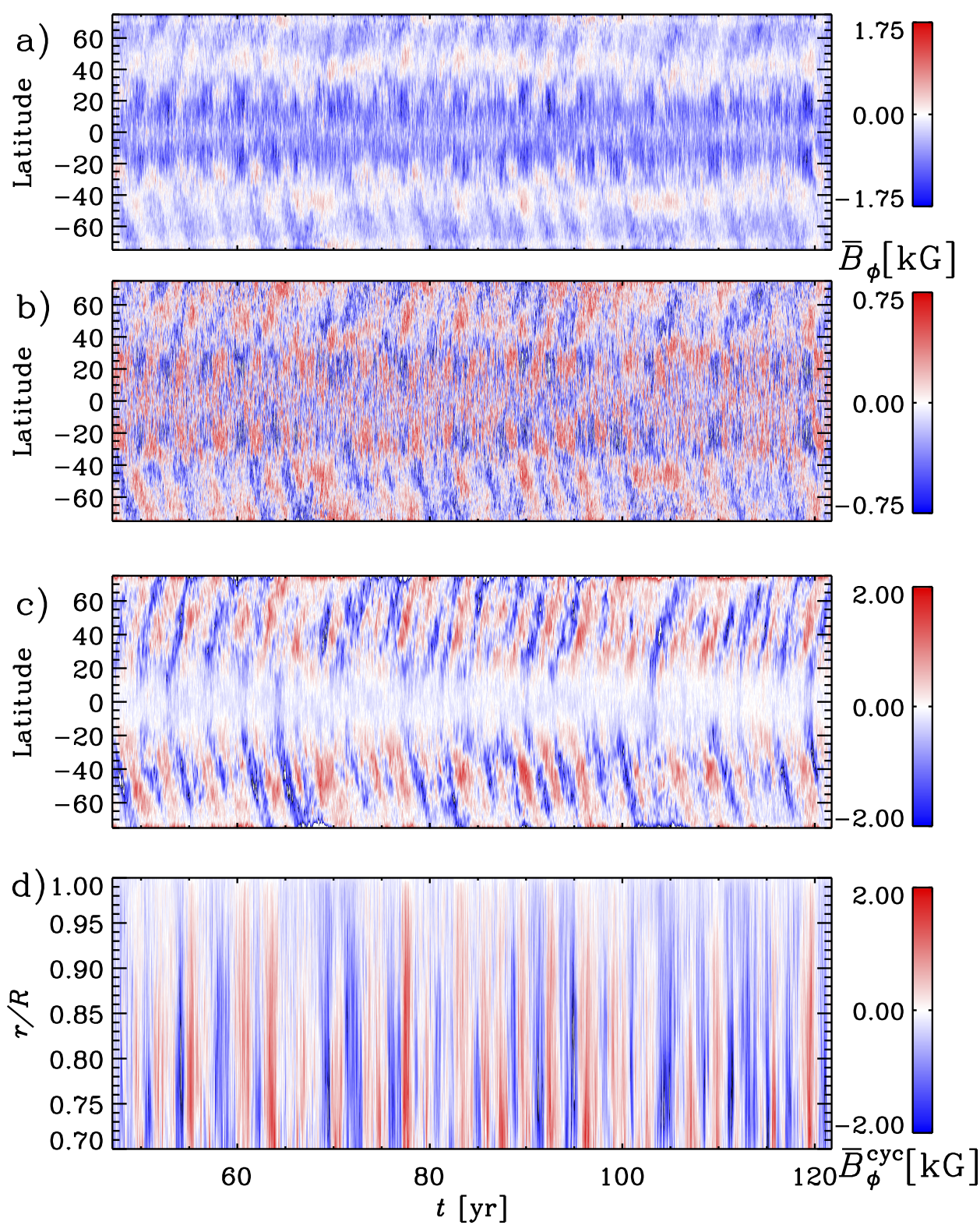
Figure 1: (a): time-latitude diagram for $\overline{B}_{\phi}$ near the surface ($r=0.98~{}R$). (b): analogously for $\overline{B}_{\phi}^{\,\rm cyc}=\overline{B}_{\phi}-\langle\overline{B}_{\phi}\rangle_{t}$. (c): same as in (b), but at $r=0.8~{}R$. (d): time-radius diagram for $\overline{B}_{\phi}^{\,\rm cyc}$ at latitude $50^{\circ}$.

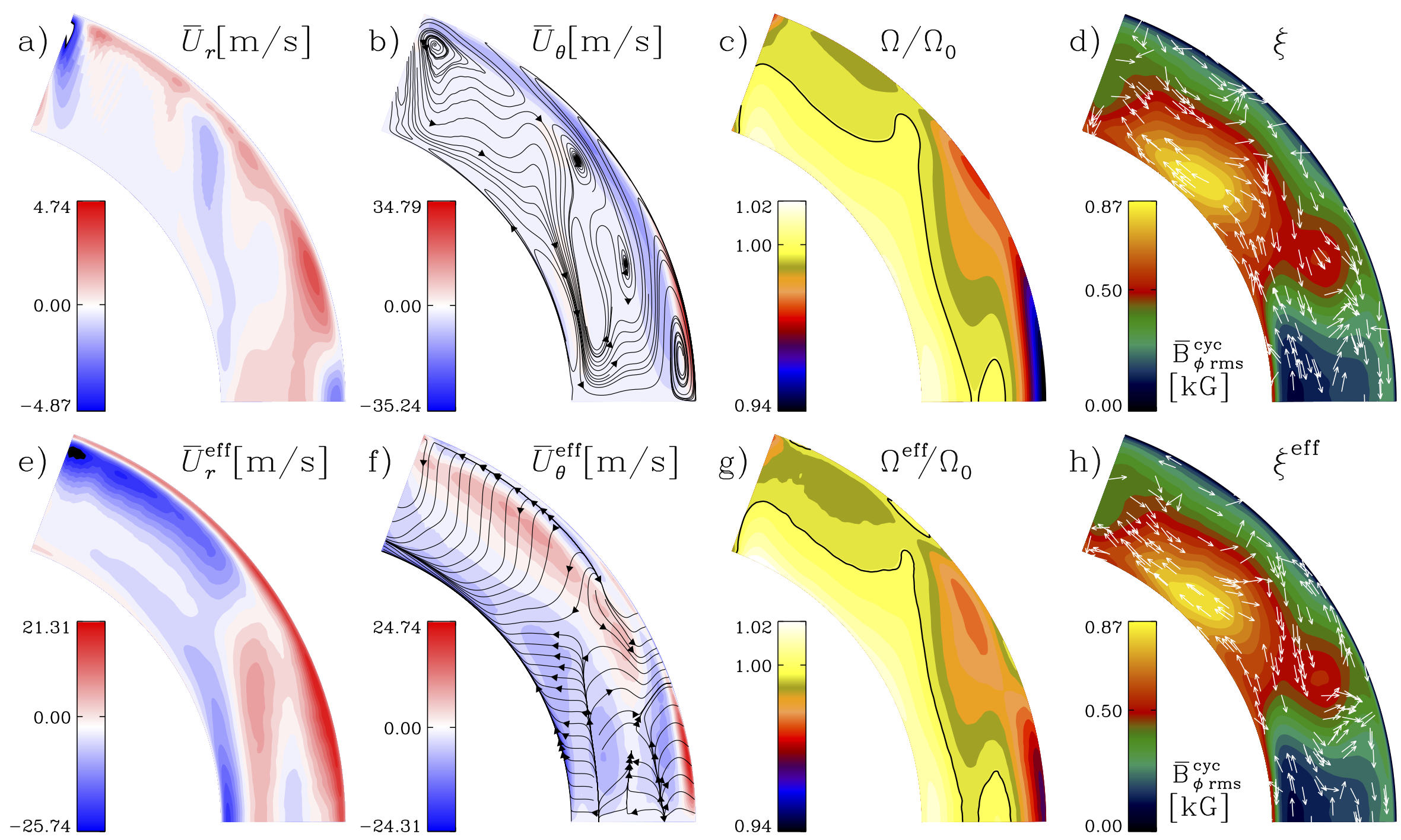
Figure 2: Time-averaged radial (a) and latitudinal (b) components of the meridional circulation ($\overline{U}_{r},\overline{U}_{\theta}$, 0), (c) mean angular velocity $\Omega=\overline{U}_{\phi}/r\sin\theta+\Omega_{0}$ and (d) temporal rms value of the azimuthal component of the cyclic magnetic field $\overline{B}_{\phi}^{\,\rm cyc}$. (e)-(h): same as (a)-(d), but using the effective mean velocity. Flow lines in (b), (f): meridional and effective meridional circulation, respectively. Black lines in (c) and (g): $\Omega/\Omega_{0}=1$ and $\Omega^{\rm eff}/\Omega_{0}=1$, respectively. Arrows in d), h): direction of the Parker-Yoshimura dynamo wave propagation, see Eq. (10).

3.2 Mean flows

We start our analysis by investigating meridional circulation and DR as shown in Figure 2(a)-(c). The former has a dominant, large, anticlockwise cell, producing a relatively strong (20 m s^-1) poleward flow near the surface at almost all latitudes. There is a slow equatorward return flow widely distributed in the bulk of the convection zone at mid to high latitudes. In the slow rotation regime, anti-solar DR is often accompanied by a single cell anti-clockwise meridional circulation. In contrast, in the regime of fast rotation, solar-like DR drives multicellular meridional circulation aligned with the rotation axis. The cell pattern in this run represents a transitional state between these two regimes (e.g., Käpylä et al., 2014; Karak et al., 2015; Featherstone & Miesch, 2015).

The DR profile shows a decelerated equator and accelerated polar regions at the surface; hence it is broadly speaking anti-solar, despite some regions of weakly solar-like DR at the bottom of the CZ. The pole-equator difference at the surface is comparable to runs with similar rotational influence (e.g. Karak et al., 2015; Warnecke, 2018). However, the energy in the DR compared to the total kinetic energy, neglecting the rigid rotation, is smaller than in runs with slightly slower and faster rotation (Viviani et al., 2018). This is most likely because our run is very close to the actual AS-S transition. In the DR profile, we find two distinct features: at mid-latitudes there is a local minimum of $\Omega$, which has also been found in simulations with about three times faster rotation. In these, the resulting shear drives a dynamo wave obeying the Parker-Yoshimura rule (e.g. Warnecke et al., 2014). Furthermore, we find strong negative shear in a layer near the surface at low latitudes.

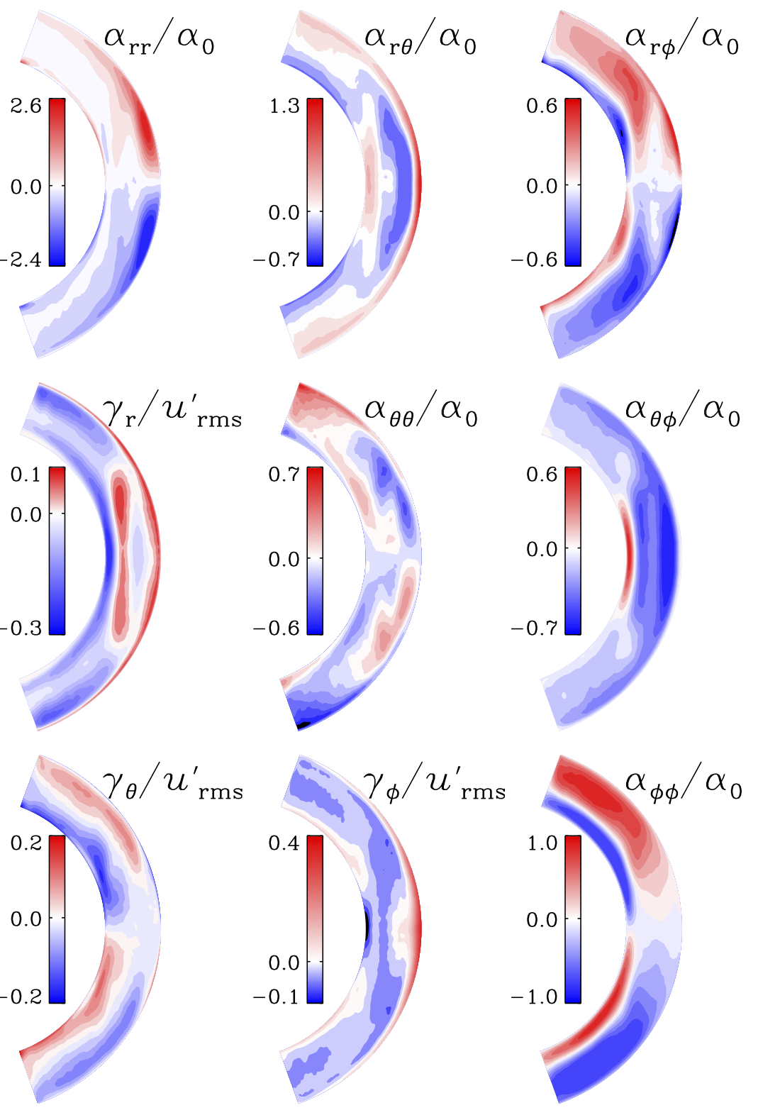
Figure 3: Independent components of time-averaged $\boldsymbol{\alpha}$, normalized by $\alpha_{0}=u^{\prime}_{{\rm rms}}/3$, and $\boldsymbol{\gamma}$, normalized by $u^{\prime}_{{\rm rms}}$.

3.3 Turbulent transport coefficients

Next, we look at the turbulent transport coefficients, for which we have used a slightly different definition than in previous work (Schrinner et al., 2007; Warnecke et al., 2018), see Appendix A for motivation and details. We begin by discussing $\boldsymbol{\alpha}$ and $\boldsymbol{\gamma}$, and compare them with their counterparts from a more rapidly rotating dynamo run with solar-like DR of Warnecke et al. (2018) in terms of the ratio of their extremal values. Regarding $\boldsymbol{\alpha}$ (see Figure 3), both $\alpha_{rr}$ and $\alpha_{\phi\phi}$ are 20 % smaller than in Warnecke et al. (2018), while the meridional profiles are similar. Furthermore, $\alpha_{\theta\theta}$ is nearly 30% larger and shows an opposite sign near the surface close to the equator. The corresponding ratios for the off-diagonal components $\alpha_{r\theta}$, $\alpha_{\theta\phi}$, and $\alpha_{r\phi}$ are 1.9, 1.1, and 0.7, respectively. Moreover, $\alpha_{r\theta}$ and $\alpha_{r\phi}$ show opposite signs at the equator near the surface. We associate these differences from Warnecke et al. (2018) with the milder rotational influence on convection, characterized by the Coriolis number, being roughly three times smaller in our run. The usage of the new definition of the turbulent transport coefficients could also have caused some of these differences, but this influence was checked to be very small by re-computing the coefficients for Warnecke et al. (2018) using the new convention. A detailed comparison is shown in Table 1 of Appendix A.

Concerning the turbulent pumping (see Figure 3), $\gamma_{r}$ has a similar magnitude, $\gamma_{\theta}$ is 40% weaker and $\gamma_{\phi}$ is 40% stronger than in Warnecke et al. (2018). Here, too, the new definition has no significant effect. Note also the different normalization we used for $\boldsymbol{\gamma}$. $\gamma_{r}$ is upward everywhere except in the bulk of the convection zone at mid and high latitudes. $\gamma_{\theta}$ is equatorward (poleward) in the upper (lower) half of the convection zone. $\gamma_{\phi}$ is prograde near the surface and at mid-latitudes near the bottom, and negative everywhere else. The magnitudes of all three components are around 0.3 $u^{\prime}_{{\rm rms}}$, where $u^{\prime}_{{\rm rms}}(r,\theta)=\langle{\boldsymbol{u}^{\prime}}^{2}\rangle^{1/2}_{\phi t}$ is the local turbulent rms velocity in the meridional plane. The effective mean velocity resulting from $\boldsymbol{\gamma}$ is shown by its time average in Figure 2(e)-(g). The radial component, $\overline{U}_{r}^{\rm eff}$, is completely dominated by $\gamma_{r}$, leaving nearly no trace of the actual flow. $\gamma_{\theta}$ changes the sign of $\overline{U}_{\theta}$ only slightly below the surface and reduces its magnitude by around 30%. However, the meridional flows cells are completely destroyed, as shown by the flow lines in Figure 2f. $\gamma_{\phi}$ is accelerating the equator and decelerating the polar region. The larger change in $\Omega^{\rm eff}$ compared to Warnecke et al. (2018) is because $\gamma_{\phi}$ increases with decreasing $\Omega_{0}$.

The reconstruction of the turbulent EMF $\overline{\boldsymbol{\cal E}}$ based on Eq. (4) shows reasonable agreement with $\overline{{\boldsymbol{u}}^{\prime}\times{\boldsymbol{b}}^{\prime}}$, see Appendix C. Therefore, we can confidently use the set of turbulent transport coefficients to describe the dynamo processes in this run.

3.4 Dynamo cycles and migration

As a first step in determining the possible dynamo mechanism, we compare the period of the magnetic field cycle with theoretical expectations. We compute the magnetic cycle period by Fourier transforming $\overline{B}_{\phi}$ at $r=0.98R$ and then averaging the spectra over latitude. As a result, we get $P_{\rm cyc}=(3.2\pm 0.3)~{}{\rm yrs}$, where the error is obtained from the width at half maximum.

The two main dynamo scenarios both make predictions for the dynamo cycle length $P_{\rm cyc}$. The Parker-Yoshimura dynamo period is locally defined as (Parker, 1955; Yoshimura, 1975)

$$P_{\rm PY}=2\pi\left|\frac{\alpha_{\phi\phi}k_{\theta}}{2}r\operatorname{cos}\theta\,\partial_{r}\Omega\right|^{-1/2},$$ (7)

where $k_{\theta}=2\pi/(r\Delta\theta)$ is the latitudinal wavenumber of the dynamo wave with $\Delta\theta=\pi/2-\theta_{0}$. The justification of using only $\alpha_{\phi\phi}$ in Eq. (7) is that the other contributions to the poloidal field generation are smaller.

The cycle period of an advection-dominated dynamo is related to the travel time of the meridional circulation from the equator to the pole, $\tau_{\rm MC}$, such that $P_{\rm MC}\approx 2\,\tau_{\rm MC}$ (Küker et al., 2001, 2019). Hence, in our notations, the expected cycle period can be written as

$$P_{\rm MC}=\frac{2r\Delta\theta}{\overline{U}_{\rm MC}(r,\theta)}$$ (8)

where $\overline{U}_{\rm MC}$ is the temporal rms of the meridional flow at the location of the dynamo wave. Traditionally, advection-dominated dynamo models assume the meridional flow and the resulting migration to be significant near the bottom of the convection zone, which would correspond to setting $r=0.7~{}R$, but in the present case it is not so straightforward to determine the location of the dynamo wave.

We start by using the measured radial DR in Eq. (7), and meridional flow in Eq. (8), and obtain for the averages over the convection zone $\langle P_{\rm PY}\rangle_{r\theta}=2.2~{}{\rm yr}$ and $\langle P_{\rm MC}\rangle_{r\theta}=8.2~{}{\rm yr}$. Using the meridional circulation in the lower quarter of the convection zone only, we obtain, instead, $\left<P_{\rm MC}\right>_{\delta r\theta}=63.8~{}{\rm yr}$, where $\delta r$ goes from $0.7R$ to $R/4$. Considering the relevant role of the turbulent pumping, especially in $\overline{U}_{r}$, we also calculated the periods using the effective velocity, that is adding the contributions of turbulent pumping to the measured large-scale flows, obtaining $\langle P_{\rm PY}^{\rm eff}\rangle_{r\theta}=2.0~{}{\rm yr}$, $\langle P_{\rm MC}^{\rm eff}\rangle_{r\theta}=5.6~{}{\rm yr}$ and $\left<P^{\rm eff}_{\rm MC}\right>_{\delta r\theta}=22.0~{}{\rm yr}$. The Parker-Yoshimura periods are less affected than those from meridional circulation, as the $\boldsymbol{\gamma}$ contribution is more significant for the meridional circulation than for the DR. In conclusion, the Parker-Yoshimura periods are consistent with the measured magnetic cycle, while advection by meridional flow cannot explain it.

If the mean magnetic field was advected by the meridional flow or its effective counterpart, one would not be able to explain poleward migration virtually everywhere within the convection zone. This becomes evident from Figure 2(b) and (f), where equatorward flows are present. Whether the meridional circulation is able to overcome diffusion, can be assessed by help of the corresponding dynamo number (or turbulent magnetic Reynolds number)

$$C_{U}=\Delta r\,\langle\overline{U}_{\rm MC}\rangle_{r\theta}/\langle{\rm Tr\!\left\{\boldsymbol{\beta}\right\}}\rangle_{r\theta},$$ (9)

where $\operatorname{Tr}\!\,\{\cdot\}$ indicates the trace. The time-averaged values for the measured mean and the effective mean flow are 0.2 and 0.6, respectively. Values below unity imply that the (effective) flow cannot overcome diffusion, not even with $\boldsymbol{\gamma}$ included; therefore, the advection-dominated dynamo scenario is not applicable here. However, the obtained values indicate that the meridional circulation may not be completely negligible in the magnetic evolution.

The prediction for the Parker-Yoshimura wave propagation direction given by (Yoshimura, 1975)

$$\boldsymbol{\xi}(r,\theta)=-\alpha_{\phi\phi}\hat{{\boldsymbol{e}}}_{\phi}\times\mbox{\boldmath$\nabla$}{}{\Omega},$$ (10)

is depicted in Figure 2d) and h) for the shear from $\Omega$ and $\Omega^{\rm eff}$, respectively. Near the bottom of the convection zone, where also the cyclic field is strongest, $\boldsymbol{\xi}$ is poleward at almost all latitudes, which would agree with the actual field propagation. In the bulk of the convection zone, however, the predicted direction is equatorward, failing to explain the actual migration. Hence, neither the Parker-Yoshimura-rule-obeying dynamo wave nor the advection dominated dynamo alone can be responsible for the oscillating magnetic field, poleward migrating throughout the convection zone.

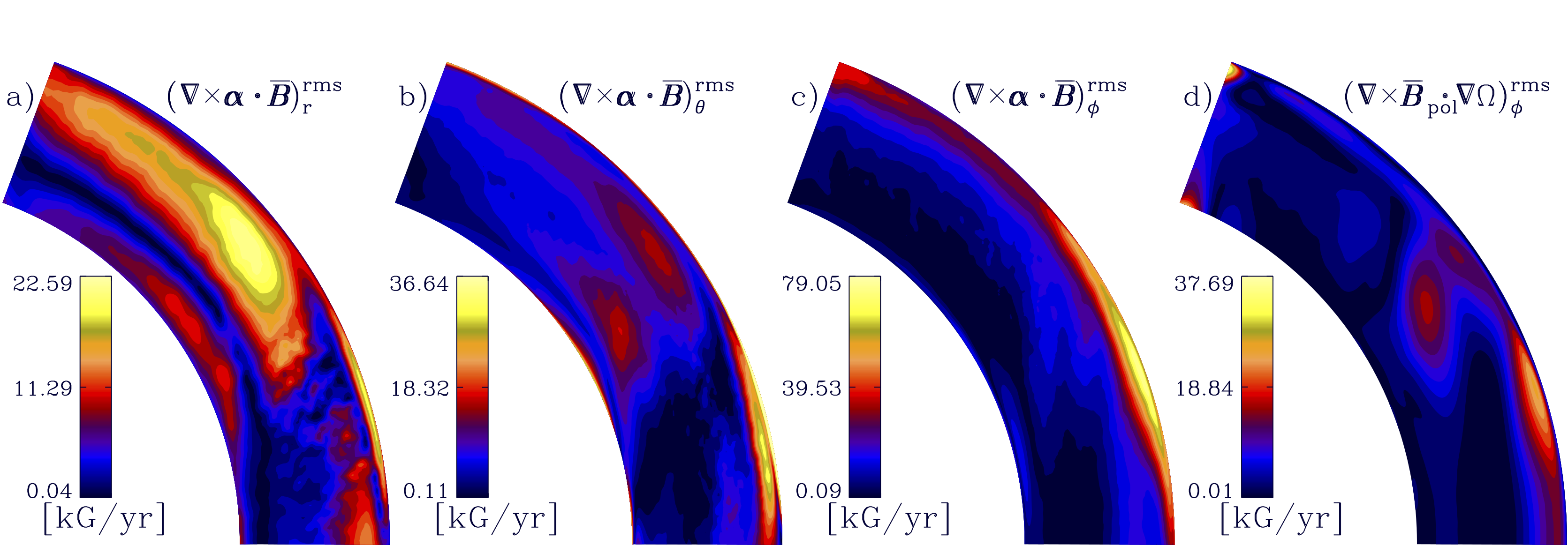
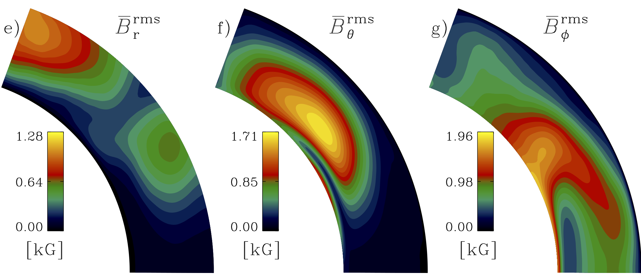
Figure 4: (a)-(d): temporal rms of the components of the $\alpha$ and $\Omega$ effect terms. (a),(b): poloidal field generators; (c),(d): toroidal field generators. (e)-(g): temporal rms values of the components of $\overline{\boldsymbol{B}}$.

3.5 Dynamo drivers

To understand the failure of the simple dynamo scenarios in explaining cycles and migration of the field, we finally turn to computing the terms contributing to the magnetic field generation in detail. We present the contributions of the $\Omega$ and $\alpha$ effects, that is, of $\overline{\boldsymbol{B}}\cdot\mbox{\boldmath$\nabla$}{}\Omega$ and $\mbox{\boldmath$\nabla$}{}\times(\boldsymbol{\alpha}\cdot\overline{\boldsymbol{B}})$, in terms of their temporal rms values in Figure 4 employing the total magnetic field (upper row), and show the corresponding temporal rms magnetic fields in the lower row. The two leftmost (rightmost) columns show the generators for the poloidal (toroidal) magnetic field. From the magnitudes of the toroidal generators, it is evident that the $\alpha$ effect is equally important, or even dominant over the $\Omega$ effect. Hence, the generation of the toroidal field by the $\alpha$ effect is more efficient than by the $\Omega$ effect, suggesting an $\alpha^{2}\Omega$ or even an $\alpha^{2}$ dynamo mechanism for the observed dynamo.

The $\Omega$ effect generates toroidal field efficiently at low latitudes near the surface and at mid-latitudes in the bulk of the convection zone, coinciding with the surroundings of the local minimum of $\Omega$. The $\alpha$ effect is strongest near the surface, but shows also toroidal field generation around the local minimum of $\Omega$. The patches of strong rms toroidal field, however, overlap only partially with its generators, and its profile is clearly offset deeper into the convection zone. One reason might be the radial-field boundary condition, which suppresses any toroidal field near the surface. The $\alpha$ effect generates poloidal field mostly at high latitudes at all depths of the convection zone, although there are also regions of strong field generation close to the surface near the equator. The high-latitude field generator profiles match qualitatively better to the rms poloidal field distribution than to that of the toroidal field, but still the match is very incomplete.

The mismatch between the generators and the actual field distribution indicates that our conclusion of the generating mechanism being a simple $\alpha^{2}\Omega$ or $\alpha^{2}$ dynamo is not a very solid one, and that other dynamo effects might be at play. For example, we find that the $\delta$ (Rädler) effect may also redound to the driving of the dynamo. Its contribution, shown in Figure 6 in Appendix A, is significant near the surface, at mid-latitudes for the poloidal field (panels a-b) and at all latitudes for the toroidal field (panel c). Particularly in the latter case, the contribution of $\boldsymbol{\delta}$ is strong in the same regions as the $\alpha$ and $\Omega$ effects and with roughly the same magnitude. However, this effect, in its simplest form in a shear flow, is known to lead to stationary solutions (Brandenburg & Subramanian, 2005). Hence, its role for the oscillatory dynamo mode is likely to be negligible. How the $\delta$ effect contributes to the magnetic field generation needs to be analyzed in detail using mean-field simulations.

The study of Warnecke (2018) covers parameter regimes very close to the one explored here, but all of these solutions appear to exhibit only stationary or temporally irregular modes. This draws attention to the role of the wedge assumption used in that study. There, the computational domain covers only $\pi/2$ in azimuth, instead of the full $2\pi$ interval here, being virtually the only difference between these two studies. Our interpretation is that there are various dynamo modes excited with very similar critical dynamo numbers. In terms of dynamo theory, the coexistence of a steady and an oscillating field constituent can be understood as follows: sufficiently overcritical flows enable the growth of more than one dynamo mode. Under the assumption of steady mean flows and statistically stationary turbulence, the time dependence of these eigenmodes is exponential with an, in general, complex increment. It is well conceivable that a non-oscillating and an oscillating mode are both excited and even continue to coexist in their nonlinear stage, although their kinematic growth rates were different.

4 Conclusions

We presented and analyzed a spherical convective dynamo simulation located in the transitional regime between S and AS rotation profiles. Unlike the oscillatory or stationary/irregular dynamos, of the S and AS regimes, the dynamo consists of coexisting cyclic and stationary modes. Metcalfe et al. (2016) suggested that the drop in the variability level of stars slightly less active than the Sun could be the result of a shutdown of the dynamo. Motivated by our finding of coexisting cyclic and stationary modes, we rather interpret this drop to be due to a change in the dynamo type. We tried to explain the oscillating magnetic field as a Parker-Yoshimura-rule-obeying dynamo wave or within the advection-dominated framework. Neither of the two approaches alone can explain the results in terms of cycle period and migration direction, even if we take the turbulent contributions to the effective mean flow into account. One reason might be that the $\alpha$ effect plays here a more dominant role than in a simple $\alpha\Omega$ dynamo. Our claim is validated by the analysis of the field generators shown in Figure 4: the mean field is generated by cyclonic convection and DR together, suggestive of an $\alpha^{2}\Omega$ or $\alpha^{2}$ dynamo. However, the spatial distributions of the generators do not match very well with those of the mean fields. This likely indicates that other dynamo effects may also play important roles, and we find evidence of a significant contribution from the $\delta$ effect. However, mean-field models that take into account all turbulent effects are needed to address this issue.

Appendix A Redefinition of the turbulent transport coefficients

A.1 Motivation

As mentioned in Schrinner et al. (2007) and Warnecke et al. (2018), there is some arbitrariness in deriving the transport coefficients (see Eq. (4)) from the (non-covariant) tensors $\tilde{\boldsymbol{a}}$ and $\tilde{\boldsymbol{b}}$ defined by

$$\overline{\cal E}_{\kappa}=\tilde{a}_{\kappa\lambda}\overline{B}_{\lambda}+\tilde{b}_{\kappa\lambda r}\partial_{r}\overline{B}_{\lambda}+\tilde{b}_{\kappa\lambda\theta}\partial_{\theta}\overline{B}_{\lambda},\quad\kappa,\lambda=r,\theta,\phi$$ (A1)

which form the immediate outcome of the test-field method. Here, we specify a choice, different from the one employed earlier (see Schrinner et al., 2007; Warnecke et al., 2018; Warnecke, 2018), and characterized by a maximum of vanishing components in $\boldsymbol{\kappa}$. As a consequence, the role of $\boldsymbol{\kappa}$ in the turbulent EMF $\overline{\boldsymbol{\cal E}}$ is reduced, while mainly that of $\boldsymbol{\beta}$ is enhanced. This is motivated by the difficulty to interpret $\boldsymbol{\kappa}$ physically, whereas $\boldsymbol{\beta}$ clearly stands for turbulent dissipation. As a meaningful side effect, the diagonal elements of the latter become equal for isotropic turbulence. Furthermore, localized appearances of negative definite $\boldsymbol{\beta}$, which are destructive to mean-field modeling, become more visible as less of the diffusive contributions (ideally none) are “hidden” in $\boldsymbol{\kappa}$. Thus, removing the negative definiteness in the redefined $\boldsymbol{\beta}$ has better prospects to render the mean-field model feasible.

A.2 Decomposition

In Eq. (A1), the components $\tilde{b}_{\kappa\lambda\phi}$ do not appear as all $\phi$ derivatives vanish. They show up in the definitions of $\boldsymbol{\alpha}$, $\boldsymbol{\beta}$, etc. though, but setting them arbitrarily cannot change $\overline{\boldsymbol{\cal E}}$. Here, we choose $\tilde{b}_{\kappa\lambda\phi}=-\tilde{b}_{\kappa\phi\lambda}$, in contrast to Schrinner et al. (2007) who set $\tilde{b}_{\kappa\lambda\phi}=0$. Then we arrive at the following expressions for the transport coefficients, where underlines indicate new or altered terms in comparison to Schrinner et al. (2007):

$$\alpha_{rr} = \tilde{a}_{rr}-\tilde{b}_{r\theta\theta}/r$$ (A2)

$$\alpha_{r\theta}=\alpha_{\theta r} = \frac{1}{2}\big{(}\tilde{a}_{r\theta}+\tilde{a}_{\theta r}+(\tilde{b}_{rr\theta}-\tilde{b}_{\theta\theta\theta})/r\big{)}$$ (A3)

$$\alpha_{r\phi}=\alpha_{\phi r} = \frac{1}{2}\big{(}\tilde{a}_{r\phi}+\tilde{a}_{\phi r}-(\underline{\tilde{b}_{r\phi r}+\cot\theta\,\tilde{b}_{r\phi\theta}}+\tilde{b}_{\phi\theta\theta})/r\big{)}$$ (A4)

$$\alpha_{\theta\theta} = \tilde{a}_{\theta\theta}+\tilde{b}_{\theta r\theta}/r$$ (A5)

$$\alpha_{\theta\phi}=\alpha_{\phi\theta} = \frac{1}{2}\big{(}\tilde{a}_{\theta\phi}+\tilde{a}_{\phi\theta}-(\underline{\tilde{b}_{\theta\phi r}+\cot\theta\,\tilde{b}_{\theta\phi\theta}}-\tilde{b}_{\phi r\theta})/r\big{)}$$ (A6)

$$\alpha_{\phi\phi} = \tilde{a}_{\phi\phi}-(\underline{\tilde{b}_{\phi\phi r}+\cot\theta\,\tilde{b}_{\phi\phi\theta}})/r$$ (A7)

$$\gamma_{r} = \frac{1}{2}\big{(}\tilde{a}_{\phi\theta}-\tilde{a}_{\theta\phi}+(\underline{\tilde{b}_{\theta\phi r}+\cot\theta\,\tilde{b}_{\theta\phi\theta}}+\tilde{b}_{\phi r\theta})/r\big{)}$$ (A8)

$$\gamma_{\theta} = \frac{1}{2}\big{(}\tilde{a}_{r\phi}-\tilde{a}_{\phi r}+(\tilde{b}_{\phi\theta\theta}-\underline{\tilde{b}_{r\phi r}-\cot\theta\,\tilde{b}_{r\phi\theta}})/r\big{)}$$ (A9)

$$\gamma_{\phi} = \frac{1}{2}\big{(}\tilde{a}_{\theta r}-\tilde{a}_{r\theta}-(\tilde{b}_{rr\theta}+\tilde{b}_{\theta\theta\theta})/r\big{)}$$ (A10)

$$\beta_{rr} = -\underline{1}\cdot\tilde{b}_{r\phi\theta}$$ (A11)

$$\beta_{r\theta}=\beta_{\theta r} = \underline{\frac{1}{2}}(\tilde{b}_{r\phi r}-\tilde{b}_{\theta\phi\theta})$$ (A12)

$$\beta_{r\phi}=\beta_{\phi r} = \frac{1}{4}(-\underline{2}\tilde{b}_{\phi\phi\theta}+\tilde{b}_{rr\theta}-\tilde{b}_{r\theta r})$$ (A13)

$$\beta_{\theta\theta} = \underline{1}\cdot\tilde{b}_{\theta\phi r}$$ (A14)

$$\beta_{\theta\phi}=\beta_{\phi\theta} = \frac{1}{4}(\underline{2}\tilde{b}_{\phi\phi r}+\tilde{b}_{\theta r\theta}-\tilde{b}_{\theta\theta r})$$ (A15)

$$\beta_{\phi\phi} = \frac{1}{2}(\tilde{b}_{\phi r\theta}-\tilde{b}_{\phi\theta r})$$ (A16)

$$\delta_{r} = \frac{1}{4}(\tilde{b}_{\theta\theta r}-\tilde{b}_{\theta r\theta}+\underline{2}\tilde{b}_{\phi\phi r})$$ (A17)

$$\delta_{\theta} = \frac{1}{4}(\tilde{b}_{rr\theta}-\tilde{b}_{r\theta r}+\underline{2}\tilde{b}_{\phi\phi\theta})$$ (A18)

$$\delta_{\phi} = \underline{-\frac{1}{2}}(\tilde{b}_{r\phi r}+\tilde{b}_{\theta\phi\theta})$$ (A19)

$$\kappa_{irr} = -\tilde{b}_{irr}$$ (A20)

$$\kappa_{ir\theta}=\kappa_{i\theta r} = -\frac{1}{2}(\tilde{b}_{ir\theta}+\tilde{b}_{i\theta r})$$ (A21)

$$\kappa_{ir\phi}=\kappa_{i\phi r} = \underline{0}$$ (A22)

$$\kappa_{i\theta\theta} = -\tilde{b}_{i\theta\theta}$$ (A23)

$$\kappa_{i\theta\phi}=\kappa_{i\phi\theta} = \underline{0}$$ (A24)

$$\kappa_{i\phi\phi} = 0$$ (A25)

The results from the new definition are shown in Figure 3 for $\boldsymbol{\alpha}$ and $\boldsymbol{\gamma}$ and in Figure 5 for the six independent components of $\boldsymbol{\beta}$, the vector $\boldsymbol{\delta}$ (first three columns), and for the nine independent nonzero components of $\boldsymbol{\kappa}$ (last three columns). $\boldsymbol{\beta}$, $\boldsymbol{\delta}$, and $\boldsymbol{\kappa}$ are normalized by $\eta_{t0}=u^{\prime}_{{\rm rms}}\alpha_{\rm MLT}H_{p}/3$, where $\alpha_{\rm MLT}=5/3$ is the mixing-length parameter and $H_{p}=-1/\partial_{r}{\rm ln}\,p$ is the pressure scale height. The terms contributing to the magnetic field evolution from the $\delta$ (Rädler) effect, using the new definition, are shown in Figure 6.

Appendix B Comparison of the turbulent transport coefficients to Warnecke et al. (2018)

Table 1: Comparison with Warnecke et al. (2018). $q$ is the ratio of the respective extremal value from the present study to that of Warnecke et al. (2018).

$$\begin{array}[]{p{0.05\linewidth}c@{\hspace{3mm}}l|cc@{\hspace{3mm}}l|cc@{\hspace{3mm}}l}\hline\cr\hline\cr\vskip 3.0pt plus 1.0pt minus 1.0pt\cr{\rm Coeff}&{q}\hfil\hskip 8.53581pt&{\rm Comments}&{\rm Coeff}&{q}\hfil\hskip 8.53581pt&{\rm Comments}&{\rm Coeff}&{q}\hfil\hskip 8.53581pt&{\rm Comments}\\[2.84526pt] \hline\cr$\alpha_{rr}$&0.8\hfil\hskip 8.53581pt&&\beta_{rr}&2.4\hfil\hskip 8.53581pt&&\kappa_{rrr}&2.9\hfil\hskip 8.53581pt&\\ $\alpha_{r\theta}$&1.9\hfil\hskip 8.53581pt&\rm opposite~{}sign&\beta_{r\theta}&2.5\hfil\hskip 8.53581pt&\rm opposite~{}sign&\kappa_{rr\theta}&2.3\hfil\hskip 8.53581pt&\\[-2.84526pt] &\hfil\hskip 8.53581pt&\rm below~{}surface&&\hfil\hskip 8.53581pt&\rm in~{}deep~{}CZ&&\hfil\hskip 8.53581pt&\\ $\alpha_{r\phi}$&0.7\hfil\hskip 8.53581pt&\rm opposite~{}sign~{}near&\beta_{r\phi}&2.9\hfil\hskip 8.53581pt&&\kappa_{r\theta\theta}&3.5\hfil\hskip 8.53581pt&\rm negative~{}near\\[-2.84526pt] &\hfil\hskip 8.53581pt&\rm equator~{}in~{}upper~{}CZ&&\hfil\hskip 8.53581pt&&&\hfil\hskip 8.53581pt&\rm surface\\ $\alpha_{\theta\theta}$&1.2\hfil\hskip 8.53581pt&\rm opposite~{}sign&\beta_{\theta\theta}&4.5\hfil\hskip 8.53581pt&\rm weakly~{}negative~{}layer&\kappa_{\theta rr}&7.0\hfil\hskip 8.53581pt&\\[-2.84526pt] &\hfil\hskip 8.53581pt&&&\hfil\hskip 8.53581pt&\rm at~{}surface&&\hfil\hskip 8.53581pt&\\ $\alpha_{\theta\phi}$&1.1\hfil\hskip 8.53581pt&&\beta_{\theta\phi}&5.0\hfil\hskip 8.53581pt&\rm opposite~{}sign&\kappa_{\theta r\theta}&3.7\hfil\hskip 8.53581pt&\rm opposite~{}sign\\[-2.84526pt] &\hfil\hskip 8.53581pt&&&\hfil\hskip 8.53581pt&\rm near~{}surface&&\hfil\hskip 8.53581pt&\rm near~{}surface\\ $\alpha_{\phi\phi}$&0.8\hfil\hskip 8.53581pt&&\beta_{\phi\phi}&1.1\hfil\hskip 8.53581pt&&\kappa_{\theta\theta\theta}&6.5\hfil\hskip 8.53581pt&\\ $\gamma_{r}$&1.0\hfil\hskip 8.53581pt&&\delta_{r}&4\hfil\hskip 8.53581pt&\rm opposite~{}sign&\kappa_{\phi rr}&1.1\hfil\hskip 8.53581pt&\rm opposite~{}sign\\[-2.84526pt] &\hfil\hskip 8.53581pt&&&\hfil\hskip 8.53581pt&\rm at~{}surface&&\hfil\hskip 8.53581pt&\\ $\gamma_{\theta}$&0.6\hfil\hskip 8.53581pt&&\delta_{\theta}&2.4\hfil\hskip 8.53581pt&&\kappa_{\phi r\theta}&1.0\hfil\hskip 8.53581pt&\rm negative~{}layer\\[-2.84526pt] &\hfil\hskip 8.53581pt&&&\hfil\hskip 8.53581pt&&&\hfil\hskip 8.53581pt&\rm at~{}surface\\ $\gamma_{\phi}$&1.4\hfil\hskip 8.53581pt&&\delta_{\phi}&3.3\hfil\hskip 8.53581pt&&\kappa_{\phi\theta\theta}&1.4\hfil\hskip 8.53581pt&\\[2.84526pt] \hline\cr\end{array}$$

We summarize the ratios of the turbulent transport coefficients from this study and their corresponding values from Warnecke et al. (2018) in Table 1. Note that all coefficients except $\beta_{\phi\phi}$ and the nonvanishing components of $\boldsymbol{\kappa}$ are affected by the redefinition explained in Appendix A, and $\beta_{rr}$ and $\beta_{\theta\theta}$ are now twice as large as with the old definition. The extrema of the $\beta_{ij}$ are between 2.4 and 5 times larger than the ones in Warnecke et al. (2018), with only $\beta_{\phi\phi}$ having the same order of magnitude, while all the components of $\boldsymbol{\delta}$ are between 2.4 and 4 times larger. The diagonal components of $\boldsymbol{\beta}$ all show positive values throughout the domain, except for a thin layer near the surface for $\beta_{\theta\theta}$. $\beta_{r\theta}$ is positive at high latitudes and shows a sign reversal at the bottom of the convection zone at low latitudes. $\beta_{\theta\phi}$ is symmetric about the equator and changes sign in depth. $\beta_{r\phi}$ has a positive layer outside the tangent cylinder and is near zero everywhere else.

$\delta_{r}$ changes sign at high latitudes and, with respect to $\delta_{r}$ in Warnecke et al. (2018), has the opposite sign at low latitudes near the surface. Like $\beta_{r\phi}$, $\delta_{\theta}$ has also a positive layer outside the tangent cylinder and two negative patches are present, roughly at the same location as the minimum in $\Omega$. $\delta_{\phi}$ is 1.5 times larger than by the old definition.

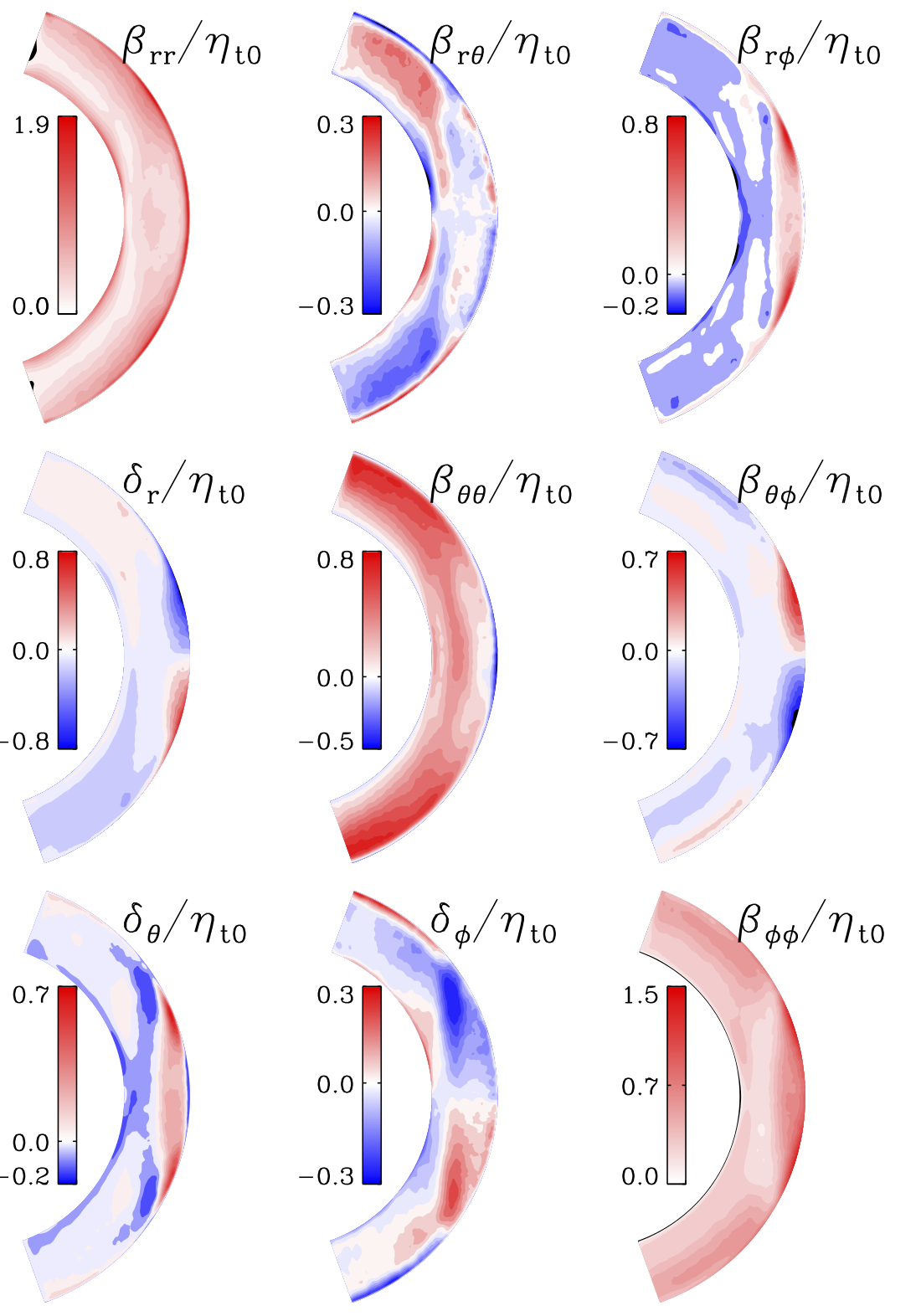
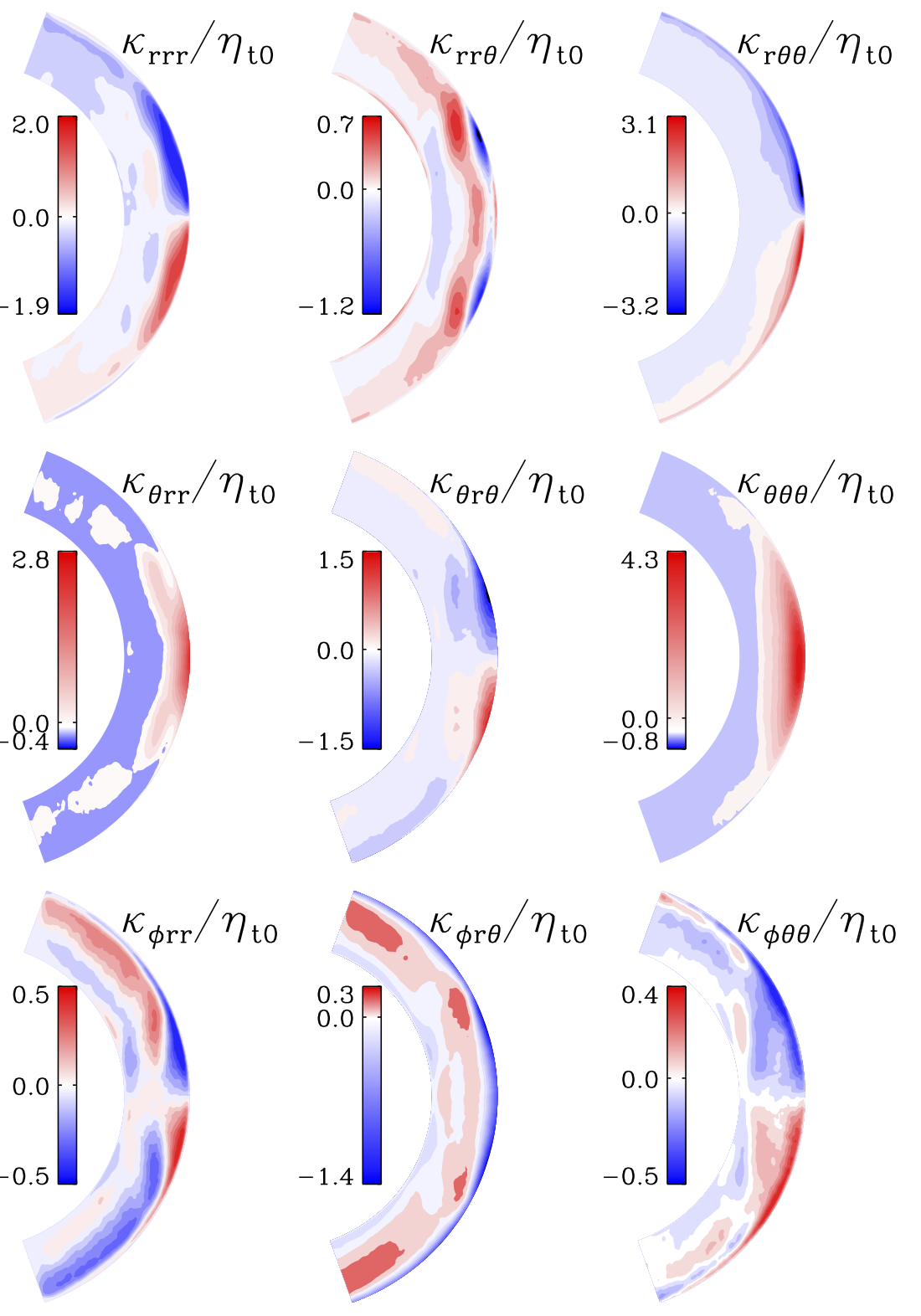
Figure 5: Independent components of time-averaged $\boldsymbol{\beta}$ and $\boldsymbol{\delta}$ (first three columns), and the nine independent components of time-averaged $\boldsymbol{\kappa}$ (last three columns), normalized by $\eta_{t0}=u^{\prime}_{{\rm rms}}\alpha_{\rm MLT}H_{p}/3$,

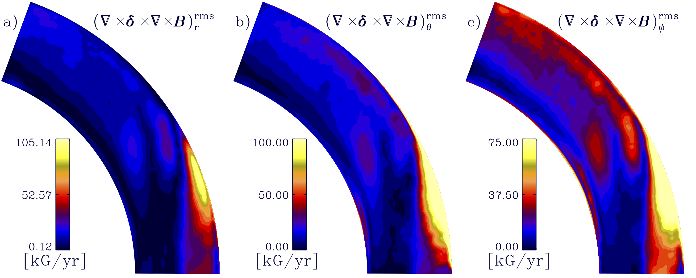
Figure 6: Temporal rms of the components of the $\delta$ (Rädler) effect, $\mbox{\boldmath$\nabla$}{}\times\boldsymbol{\delta}\times\mbox{\boldmath$\nabla$}{}\times\overline{\boldsymbol{B}}$, see Eq. (4).

The $\boldsymbol{\kappa}$ components look, in general, smoother than in Warnecke et al. (2018). Most of the $\kappa_{ijk}$ are now zero, leaving just nine independent nonzero components. $\kappa_{rrr}$, $\kappa_{rr\theta}$, $\kappa_{\theta r\theta}$ and $\kappa_{r\theta\theta}$ are roughly three times larger, $\kappa_{\phi\theta\theta}$ and $\kappa_{\phi r\theta}$ have similar magnitudes, while $\kappa_{\theta rr}$ and $\kappa_{\theta\theta\theta}$ are 7 and 6.5 times larger in the current study, respectively. $\kappa_{rr\theta}$ shows sign reversal near the surface, and $\kappa_{r\theta\theta}$ does not show any particular structure in the bulk of the convection zone, as was the case in Warnecke et al. (2018), too. $\kappa_{\theta rr}$ has strong positive values near the equator in the upper part of the convection zone, extending to mid-latitudes, while $\kappa_{\theta r\theta}$ is anti-symmetric with respect to the equator, and has the opposite sign near the surface with respect to Warnecke et al. (2018). Two sign reversals in depth are visible in $\kappa_{\phi rr}$, and also $\kappa_{\phi r\theta}$ shows three layers in depth: two narrow negative ones at the top and bottom of the convection zone and a weakly positive one in the bulk.

While $\boldsymbol{\alpha}$ and $\boldsymbol{\gamma}$ do not differ markedly between the compared runs, the other tensors show variations by up to a factor of seven compared to Warnecke et al. (2018). Given that the roughly three-times higher Coriolis number of their run is virtually the only relevant difference to our present run, we have to assign these changes to the effect of rotational quenching (see, e.g. Kitchatinov et al., 1994). This is supported by the findings of Brandenburg et al. (2012) for rotating homogeneous turbulence who report on a reduction of $\boldsymbol{\beta}$ and $\boldsymbol{\delta}$ by a factor of approximately three when ${\rm Co}$ is increased from two to eight, with an even stronger reduction in $\boldsymbol{\kappa}$.

Appendix C Reconstruction of the turbulent electromotive force

We show in Figure 7 the turbulent EMF, computed directly via $\overline{{\boldsymbol{u}}^{\prime}\times{\boldsymbol{b}}^{\prime}}$ and its reconstruction using Eq. (4) with the time-averaged transport coefficients and the full $\overline{\boldsymbol{B}}$ during roughly five typical dynamo cycles. In the reconstructed and directly computed EMFs, we have filtered out the time average and all time-scales shorter than one year to highlight the oscillating pattern. The spatial and temporal structures of all components of the reconstructed EMF match the measured ones reasonably well. In Warnecke et al. (2018), a good match was found in the mid and high latitudes, while the near-equator behaviour was captured less accurately. However, the time average was not removed there. Now we find good correspondence also at the equatorial regions. As in Warnecke et al. (2018), the magnitudes of the reconstructed EMF components tend to be overestimated. Here, this effect is most pronounced for the azimuthal component of the EMF, which is by a factor of 2.5 larger than the measured one. This can be interpreted as a consequence of non-localities in turbulent convection, and calls for the application of scale dependent test fields to the problem.

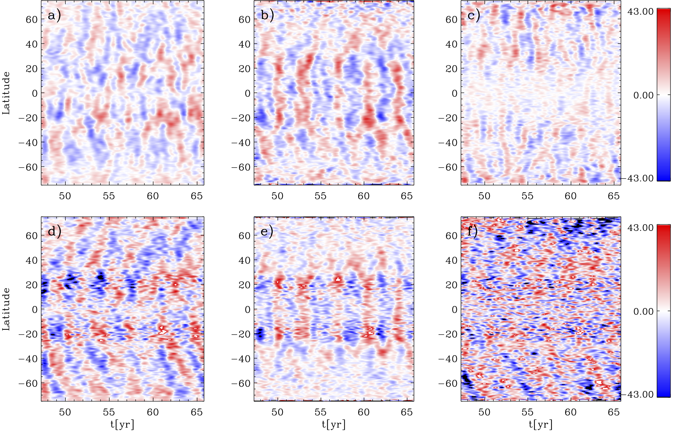
Figure 7: Radial, latitudinal, and longitudinal components of the turbulent electromotive force computed directly using $\overline{{\boldsymbol{u}}^{\prime}\times{\boldsymbol{b}}^{\prime}}$ (panels a-c) and of its reconstruction using Eq. (4) (panels d-f) near the surface ($r=0.98\,R$). Time averages and time-scales shorter than one year have been filtered out. The longitudinal components (panels c) and f)) have been multiplied by a factor 2.5.

References

- Augustson et al. (2015) Augustson, K., Brun, A. S., Miesch, M., & Toomre, J. 2015, ApJ, 809, 149
- Baryshnikova & Shukurov (1987) Baryshnikova, I., & Shukurov, A. 1987, AN, 308, 89
- Brandenburg (2017) Brandenburg, A. 2017, A&A, 598, A117
- Brandenburg & Giampapa (2018) Brandenburg, A., & Giampapa, M. S. 2018, ApJ, 855, L22
- Brandenburg et al. (2012) Brandenburg, A., Rädler, K.-H., & Kemel, K. 2012, A&A, 539, A35
- Brandenburg & Subramanian (2005) Brandenburg, A., & Subramanian, K. 2005, Phys. Rep., 417, 1
- Choudhuri et al. (1995) Choudhuri, A. R., Schüssler, M., & Dikpati, M. 1995, A&A, 303, L29
- Dikpati & Charbonneau (1999) Dikpati, M., & Charbonneau, P. 1999, ApJ, 518, 508
- Featherstone & Miesch (2015) Featherstone, N. A., & Miesch, M. S. 2015, ApJ, 804, 67
- Gastine et al. (2014) Gastine, T., Yadav, R. K., Morin, J., Reiners, A., & Wicht, J. 2014, MNRAS, 438, L76
- Gent et al. (2017) Gent, F. A., Käpylä, M. J., & Warnecke, J. 2017, Astronomische Nachrichten, 338, 885
- Käpylä et al. (2016) Käpylä, M. J., Käpylä, P. J., Olspert, N., et al. 2016, A&A, 589, A56
- Käpylä et al. (2019) Käpylä, P. J., Gent, F. A., Olspert, N., Käpylä, M. J., & Brandenburg, A. 2019, Geophys. Astrophys. Fluid Dyn., in press, arXiv:1807.09309
- Käpylä et al. (2014) Käpylä, P. J., Käpylä, M. J., & Brandenburg, A. 2014, A&A, 570, A43
- Käpylä et al. (2017) Käpylä, P. J., Käpylä, M. J., Olspert, N., Warnecke, J., & Brandenburg, A. 2017, A&A, 599, A5
- Käpylä et al. (2006) Käpylä, P. J., Korpi, M. J., & Tuominen, I. 2006, Astron. Nachr., 327, 884
- Käpylä et al. (2012) Käpylä, P. J., Mantere, M. J., & Brandenburg, A. 2012, ApJ, 755, L22
- Käpylä et al. (2013) Käpylä, P. J., Mantere, M. J., Cole, E., Warnecke, J., & Brandenburg, A. 2013, ApJ, 778, 41
- Karak et al. (2015) Karak, B. B., Käpylä, P. J., Käpylä, M. J., et al. 2015, A&A, 576, A26
- Kichatinov (1991) Kichatinov, L. L. 1991, A&A, 243, 483
- Kitchatinov et al. (1994) Kitchatinov, L. L., Pipin, V. V., & Rüdiger, G. 1994, Astron. Nachr., 315, 157
- Krause & Rädler (1980) Krause, F., & Rädler, K.-H. 1980, Mean-field Magnetohydrodynamics and Dynamo Theory (Oxford: Pergamon Press)
- Küker et al. (2019) Küker, M., Rüdiger, G., Olah, K., & Strassmeier, K. G. 2019, A&A, 622, A40
- Küker et al. (2001) Küker, M., Rüdiger, G., & Schultz, M. 2001, A&A, 374, 301
- Mabuchi et al. (2015) Mabuchi, J., Masada, Y., & Kageyama, A. 2015, ApJ, 806, 10
- Masada & Sano (2014) Masada, Y., & Sano, T. 2014, ApJ, 794, L6
- Metcalfe et al. (2016) Metcalfe, T. S., Egeland, R., & van Saders, J. 2016, ApJ, 826, L2
- Mitra et al. (2010) Mitra, D., Tavakol, R., Käpylä, P. J., & Brandenburg, A. 2010, ApJ, 719, L1
- Olspert et al. (2018) Olspert, N., Lehtinen, J. J., Käpylä, M. J., Pelt, J., & Grigorievskiy, A. 2018, A&A, 619, A6
- Ossendrijver et al. (2002) Ossendrijver, M., Stix, M., Brandenburg, A., & Rüdiger, G. 2002, A&A, 394, 735
- Parker (1955) Parker, E. N. 1955, ApJ, 121, 491
- Rädler & Bräuer (1987) Rädler, K.-H., & Bräuer, H.-J. 1987, Astron. Nachr., 308, 101
- Schrinner (2011) Schrinner, M. 2011, A&A, 533, A108
- Schrinner et al. (2011) Schrinner, M., Petitdemange, L., & Dormy, E. 2011, A&A, 530, A140
- Schrinner et al. (2012) —. 2012, ApJ, 752, 121
- Schrinner et al. (2005) Schrinner, M., Rädler, K.-H., Schmitt, D., Rheinhardt, M., & Christensen, U. 2005, Astron. Nachr., 326, 245
- Schrinner et al. (2007) Schrinner, M., Rädler, K.-H., Schmitt, D., Rheinhardt, M., & Christensen, U. R. 2007, Geophys. Astrophys. Fluid Dynam., 101, 81
- Strugarek et al. (2017) Strugarek, A., Beaudoin, P., Charbonneau, P., Brun, A. S., & do Nascimento, J.-D. 2017, Science, 357, 185
- Viviani et al. (2018) Viviani, M., Warnecke, J., Käpylä, M. J., et al. 2018, A&A, 616, A160
- Warnecke (2018) Warnecke, J. 2018, A&A, 616, A72
- Warnecke et al. (2014) Warnecke, J., Käpylä, P. J., Käpylä, M. J., & Brandenburg, A. 2014, ApJ, 796, L12
- Warnecke et al. (2016) —. 2016, A&A, 596, A115
- Warnecke et al. (2018) Warnecke, J., Rheinhardt, M., Tuomisto, S., et al. 2018, A&A, 609, A151
- Yoshimura (1975) Yoshimura, H. 1975, ApJ, 201, 740