Enhanced stellar activity for slow antisolar differential rotation?

Abstract

High precision photometry of solar-like members of the open cluster M67 with Kepler/K2 data has recently revealed enhanced activity for stars with a large Rossby number, which is the ratio of rotation period to the convective turnover time. Contrary to the well established behavior for shorter rotation periods and smaller Rossby numbers, the chromospheric activity of the more slowly rotating stars of M67 was found to increase with increasing Rossby number. Such behavior has never been reported before, although it was theoretically predicted to emerge as a consequence of antisolar differential rotation (DR) for stars with Rossby numbers larger than that of the Sun, because in those models the absolute value of the DR was found to exceed that for solar-like DR. Using gyrochronological relations and an approximate age of $4\,{\rm Gyr}$ for the members of M67, we compare with computed rotation rates using just the $B-V$ color. The resulting rotation–activity relation is found to be compatible with that obtained by employing the measured rotation rate. This provides additional support for the unconventional enhancement of activity at comparatively low rotation rates and the possible presence of antisolar differential rotation.

1. Introduction

Main sequence stars with outer convection zones have long displayed a remarkable universality regarding their dependence of normalized chromospheric activity on their normalized rotation rate. This dependence is evident over a broad range of activity indicators including X-ray, H$\alpha$, and, in particular, the normalized chromospheric Ca ii H+K line emission, $R^{\prime}_{\rm HK}$ (e.g., Vilhu, 1984; Noyes et al., 1984). To compare late-type stars of different spectral type, these and other investigators since then normalized the rotation period $P_{\rm rot}$ by the star’s convective turnover time $\tau$, as determined from conventional mixing length theory. This step is obviously model-dependent, but different prescriptions for $\tau$ as a function of $B-V$ all have in common that $\tau$ increases monotonically with $B-V$. With this normalization, the rotation–activity relations of stars of different spectral type collapse onto a universal curve. Empirically, the most useful prescription for the function $\tau(B-V)$ is one that minimizes the scatter of $R^{\prime}_{\rm HK}$ as a function of $\tau/P_{\rm rot}$, i.e., the inverse Rossby number.

For $\tau/P_{\rm rot}\ll 1$ (slow rotation), the activity indicator $R^{\prime}_{\rm HK}$ increases approximately linearly with $\tau/P_{\rm rot}$, but saturates for $\tau/P_{\rm rot}\gg 1$. In this Letter, we focus on a new behavior for values of $\tau/P_{\rm rot}$ that are smaller than what was usually considered in earlier investigations. In this regime, Giampapa et al. (2017) found that $R^{\prime}_{\rm HK}$ increases with decreasing values of $\tau/P_{\rm rot}$. The same trend is reproduced when using the earlier $R^{\prime}_{\rm HK}$ values of Giampapa et al. (2006) at somewhat higher spectral resolution where the effects of color-dependent contamination from the line wings is smaller. Also calibration uncertainties were shown to be small.

The unconventional scaling of $R^{\prime}_{\rm HK}$ with $\tau/P_{\rm rot}$ can be associated with a theoretically predicted increase in differential rotation (DR) at Rossby numbers somewhat above the solar value, i.e., for slower rotation in the normalized sense. This is the regime of antisolar DR (slow equator, fast poles). The associated increase of magnetic energy with decreasing rotation rate was first noticed by Karak et al. (2015); see their Figure 12(b). The sign reversal of DR, however, has a much longer history and goes back to early work by Gilman (1977). More recently, with the advent of realistic high-resolution simulations of solar/stellar dynamos, it became evident that dynamo cycles could only be obtained at rotation rates that are about three times faster than that of the Sun (Brown et al., 2011). Later, Gastine et al. (2014) found hysteresis behavior in the transition from solar-like to antisolar-like DR as a function of stellar rotation rate. Solar-like DR could then be obtained for initial conditions with rapid rotation. This led Käpylä et al. (2014) to speculate that the Sun might have inherited its solar-like DR with equatorward acceleration and slow poles from its youth when it was rotating more rapidly. However, subsequent models with dynamo-generated magnetic fields by Fan & Fang (2014) did not confirm the existence of hysteresis behavior. Thus, at the solar rotation rate, simulations do indeed produce antisolar DR. This is a problem of all solar dynamo simulations to date, but it may be hoped that the qualitative trends found by Karak et al. (2015) would still hold for the Sun, but at slightly rescaled rotation rates.

The present work supports the prediction by Karak et al. (2015) of a reversed trend in the rotation–activity diagram at very low values of $\tau/P_{\rm rot}$. The purpose of this Letter is to compare the new data of Giampapa et al. (2017) with those of other stars, notably those of the Mount Wilson HK project (Baliunas et al., 1995). We focus here particularly on the main sequence stars of Brandenburg et al. (2017) (hereafter BMM) and Saar & Brandenburg (1999) (hereafter SB), for which cyclic dynamo properties have been analyzed in detail. Many of those stars have two cycle periods, which fall into one of two classes in diagrams showing the rotation-to-cycle-period-ratio versus $R^{\prime}_{\rm HK}$ or age. These properties give us a perspective on the stars’ evolutionary state in a broader context. For the stars of the Kepler sample of Giampapa et al. (2017), the time series are still too short, so no information about cyclic activity exists as yet. However, based on earlier simulations, we suggest that those stars can exhibit chaotic variability in $R^{\prime}_{\rm HK}$ by up to 0.35 dex that might be detectable over longer time spans.

Table 1 Sample of solar-like Kepler stars of Giampapa et al. (2017).

# S $B$–$V$ $T_{\rm eff}$ $\tau\;$ $P_{\rm rot}$ $P_{\rm rot}^{\ast}$ $\!\!\!\!\!\log\langle R^{\prime}_{\rm HK}\rangle\!\!\!$ age A 603 0.55 6091 6.4 $16.6$ 17.3 $-4.74$ 3.7 B 785 0.66 5757 12.6 $25.4$ 24.8 $-4.82$ 4.2 C 801 0.68 5692 13.7 $20.8$ 25.7 $-4.95$ 2.8 D 945 0.63 5856 10.8 $24.3$ 23.2 $-4.80$ 4.3 E 958 0.62 5890 10.2 $23.8$ 22.6 $-4.89$ 4.4 F 965 0.72 5564 15.9 $26.3$ 27.4 $-4.86$ 3.7 G 969 0.63 5856 10.8 $25.7$ 23.2 $-5.06$ 4.8 H 991 0.64 5823 11.4 $21.6$ 23.7 $-4.84$ 3.4 I 1089 0.63 5856 10.8 $24.5$ 23.2 $-4.97$ 4.4 J 1095 0.61 5923 9.7 $22.6$ 22.0 $-4.73$ 4.2 K 1096 0.62 5890 10.2 $19.5$ 22.6 $-4.86$ 3.1 L 1106 0.65 5790 12.0 $28.4$ 24.3 $-4.93$ 5.3 M 1212 0.73 5530 16.4 $24.7$ 27.8 $-4.86$ 3.3 N 1218 0.64 5823 11.4 $19.4$ 23.7 $-4.78$ 2.8 O 1252 0.59 5988 8.5 $20.3$ 20.7 $-4.72$ 3.9 P 1255 0.63 5856 10.8 $24.2$ 23.2 $-4.82$ 4.3 Q 1289 0.72 5564 15.9 $23.8$ 27.4 $-4.88$ 3.1 R 1307 0.77 5408 18.2 $22.4$ 29.2 $-4.95$ 2.5 S 1420 0.59 5988 8.5 $24.8$ 20.7 $-4.79$ 5.5 $\alpha$ 724 0.63 5856 10.8 — 23.2 $-4.79$ $4^{\ast}$ $\beta$ 746 0.67 5725 13.1 — 25.2 $-4.89$ $4^{\ast}$ $\gamma$ 770 0.64 5823 11.4 — 23.7 $-4.80$ $4^{\ast}$ $\delta$ 777 0.63 5856 10.8 — 23.2 $-4.90$ $4^{\ast}$ $\epsilon$ 802 0.68 5692 13.7 — 25.7 $-4.95$ $4^{\ast}$ $\zeta$ 829 0.59 5988 8.5 — 20.7 $-4.95$ $4^{\ast}$ $\eta$ 1004 0.72 5564 15.9 — 27.4 $-5.02$ $4^{\ast}$ $\theta$ 1033 0.57 6091 7.4 — 19.2 $-4.74$ $4^{\ast}$ $\iota$ 1048 0.65 5790 12.0 — 24.3 $-5.17$ $4^{\ast}$ $\kappa$ 1078 0.62 5890 10.2 — 22.6 $-4.95$ $4^{\ast}$ $\lambda$ 1087 0.60 5957 9.1 — 21.4 $-4.90$ $4^{\ast}$ $\mu$ 1248 0.58 6025 8.0 — 20.0 $-4.65$ $4^{\ast}$ $\nu$ 1258 0.63 5856 10.8 — 23.2 $-4.90$ $4^{\ast}$ $\xi$ 1260 0.58 6025 8.0 — 20.0 $-4.78$ $4^{\ast}$ $\pi$ 1269 0.72 5564 15.9 — 27.4 $-5.02$ $4^{\ast}$ $\rho$ 1318 0.58 6022 8.0 — 20.0 $-4.73$ $4^{\ast}$ $\sigma$ 1449 0.62 5890 10.2 — 22.6 $-5.13$ $4^{\ast}$ $\tau$ 1477 0.68 5692 13.7 — 25.7 $-4.94$ $4^{\ast}$

Table 2 F and G dwarfs (italics) and K dwarfs (roman) of BMM.

# HD/KIC $B$–$V$ $T_{\rm eff}$ $\tau\;$ $P_{\rm rot}$ $\!\!\!\log\langle R^{\prime}_{\rm HK}\rangle\!\!\!$ age a Sun 0.66 5778 12.6 $25.40$ $-4.90$ 4.6 b 1835 0.66 5688 12.6 $7.78$ $-4.43$ 0.5 c 17051 0.57 6053 7.5 $8.50$ $-4.60$ 0.6 d 20630 0.66 5701 12.6 $9.24$ $-4.42$ 0.7 e 30495 0.63 5780 10.9 $11.36$ $-4.49$ 1.1 f 76151 0.67 5675 13.2 $15.00$ $-4.66$ 1.6 g 78366 0.63 5915 10.9 $9.67$ $-4.61$ 0.8 h 100180 0.57 5942 7.5 $14.00$ $-4.92$ 2.3 i 103095 0.75 5035 17.4 $31.00$ $-4.90$ 4.6 j 114710 0.58 5970 8.0 $12.35$ $-4.75$ 1.7 k 128620 0.71 5809 15.4 $22.50$ $-5.00$ 5.4 l 146233 0.65 5767 12.0 $22.70$ $-4.93$ 4.1 m 152391 0.76 5420 17.8 $11.43$ $-4.45$ 0.8 n 190406 0.61 5847 9.7 $13.94$ $-4.80$ 1.8 o 8006161 0.84 5488 20.6 $29.79$ $-5.00$ 4.6 p 10644253 0.59 6045 8.6 $10.91$ $-4.69$ 0.9 q 186408 0.64 5741 11.5 $23.80$ $-5.10$ 7.0 r 186427 0.66 5701 12.6 $23.20$ $-5.08$ 7.0 a 3651 0.84 5128 20.6 $44.00$ $-4.99$ 7.2 b 4628 0.89 5035 21.7 $38.50$ $-4.85$ 5.3 c 10476 0.84 5188 20.6 $35.20$ $-4.91$ 4.9 d 16160 0.98 4819 22.8 $48.00$ $-4.96$ 6.9 e 22049 0.88 5152 21.5 $11.10$ $-4.46$ 0.6 f 26965 0.82 5284 20.1 $43.00$ $-4.87$ 7.2 g 32147 1.06 4745 23.5 $48.00$ $-4.95$ 6.4 h 81809 0.80 5623 19.4 $40.20$ $-4.92$ 6.6 i 115404 0.93 5081 22.3 $18.47$ $-4.48$ 1.4 j 128621 0.88 5230 21.5 $36.20$ $-4.93$ 4.8 k 149661 0.80 5199 19.4 $21.07$ $-4.58$ 2.1 l 156026 1.16 4600 24.2 $21.00$ $-4.66$ 1.3 m 160346 0.96 4797 22.7 $36.40$ $-4.79$ 4.4 n 1653411 0.78 5023 18.6 $19.90$ $-4.55$ 2.0 o 166620 0.90 5000 21.9 $42.40$ $-4.96$ 6.2 p 201091 1.18 4400 24.4 $35.37$ $-4.76$ 3.3 q 201092 1.37 4040 25.9 $37.84$ $-4.89$ 3.2 r 2198341 0.80 5461 19.4 $42.00$ $-5.07$ 7.1 s 2198342 0.91 5136 22.1 $43.00$ $-4.94$ 6.2 1 141004 0.60 5870 9.1 25.80 $-5.00$ 5.6 2 161239 0.65 5640 12.0 29.20 $-5.16$ 5.5 3 187013 0.47 6455 3.1 8.00 $-4.79$ — 4 224930 0.67 5470 13.1 33.00 $-4.88$ 6.4

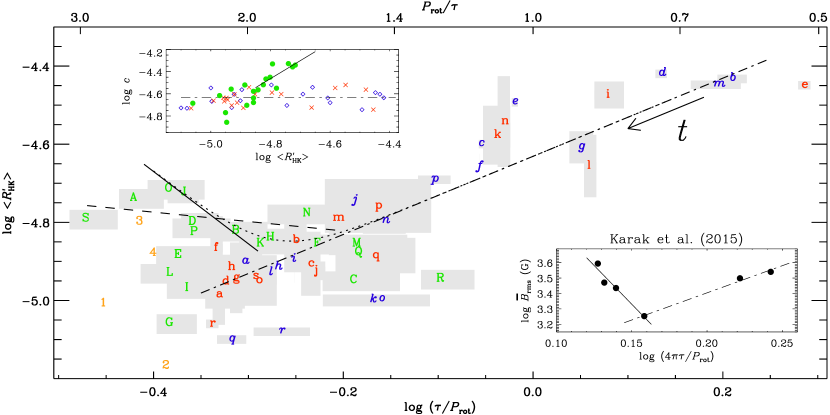
Figure 1.— $\log\langle R^{\prime}_{\rm HK}\rangle$ versus $\log(\tau/P_{\rm rot})$ for the stars of M67 with known rotation periods as green uppercase letters, the F and G dwarfs of BMM as blue italics characters, the K dwarfs of BMM as red roman characters, and the four stars of SB with $P_{\rm rot}/\tau\geq 2.4$ as orange numbers 1–4. On the upper abscissa, the Rossby number $P_{\rm rot}/\tau$ is given. The dashed-dotted line shows the fit of BMM, whereas the solid line represents a fit to the residuals in Equation (5) for the nine stars with $\log\langle R^{\prime}_{\rm HK}\rangle\geq-4.85$. The dashed line is a direct fit to the same nine stars and the dotted line shows the fit given by Equation (6). The arrow indicates the anticipated evolution with increasing age $t$. Some of the symbols have been shifted slightly to avoid overlap. The Sun corresponds to the blue italics $a$. The upper inset shows the residual $\log c$ versus $\log\langle R^{\prime}_{\rm HK}\rangle$ for the stars of M67 as green filled circles, the F and G dwarfs of BMM as blue diamonds, and the K dwarfs of BMM as red crosses. The lower inset shows the increasing magnetic field strength for small values of $4\pi\tau/P_{\rm rot}$ from Figure 12(b) of Karak et al. (2015).

2. Representation of the data

To be able to discuss individual stars in their rotation–activity diagrams, we denote the stars of M67 by uppercase roman and lowercase Greek characters and identify them by their Sanders number S in Table LABEL:TSum1. The F and G dwarfs of BMM, represented by lowercase italics characters, their K dwarfs, indicated by lowercase roman characters, and the four stars of SB with $P_{\rm rot}/\tau\geq 2.4$, indicated by the numbers 1–4, are identified by their HD or KIC numbers in Table LABEL:TSum2. In addition to $B-V$, $P_{\rm rot}$, and $R^{\prime}_{\rm HK}$, we also give in both tables the effective temperature $T_{\rm eff}$ and, for $B-V>0.495$, the gyrochronological age $t$ from the relations of Mamajek & Hillenbrand (2008),

$$t=\left\{P_{\rm rot}/[0.407\,(B-V-0.495)^{0.325}]\right\}^{1.767};$$ (1)

see also Equation (9) of BMM. Equation (1) can be inverted to compute instead $P_{\rm rot}$ under the reasonable assumption that $t=4\,{\rm Gyr}$ is valid for all stars of M67; evidence comes from isochrones (Sarajedini et al., 2009; Önehag et al., 2011), gyrochronology (Barnes et al., 2016), and chromospheric activity combined with gyrochronology (Giampapa et al., 2017). This yields

$$P_{\rm rot}^{\ast}=0.407\,(B-V-0.495)^{0.325}\;t^{0.565},$$ (2)

where the asterisk is used to distinguish the computed value from the measured one. Next, using the semi-empirical relationship for $\tau(B-V)$ of Noyes et al. (1984) in the form

$$\log\tau=1.362-0.166x+0.03x^{2}-5.3x^{3},$$ (3)

with $x=1-(B-V)$ and for $B-V<1$, we obtain $\tau/P_{\rm rot}^{\ast}$ as a monotonically increasing function of $B-V$ in the range from $0.55$ to $0.8$.

Given these relations, we first show in Figure 1 all stars with measured rotation periods in the rotation–activity diagram. Error bars in $\langle R^{\prime}_{\rm HK}\rangle$ and $P_{\rm rot}$ are marked by gray boxes. The stars of BMM follow an approximately linear increase that can be described by the fit $\log\langle R^{\prime}_{\rm HK}\rangle\approx\log(\tau/P_{\rm rot})+\log c$, where $\log c\approx-4.63$. However, in spite of significant scatter, there is a clear increase in activity for most of the stars of the sample of M67 as $\tau/P_{\rm rot}$ decreases. HD 187013 and 224930 (orange symbols 3 and 4 with $P_{\rm rot}/\tau=2.6$ and $2.5$, respectively) of the Mount Wilson stars are found to be compatible with this trend. We show two separate fits in Figure 1, a direct one and one that has been computed from a fit to the residual between $\log\langle R^{\prime}_{\rm HK}\rangle$ and $\log(\tau/P_{\rm rot})$, i.e.,

$$\log\langle R^{\prime}_{\rm HK}\rangle-\log(\tau/P_{\rm rot})=\log c_{1}+\rho\log\langle R^{\prime}_{\rm HK}\rangle.$$ (4)

In the upper inset of Figure 1 we denote this residual by $\log c$, where $c$ is a function of $\langle R^{\prime}_{\rm HK}\rangle$. Equation (4) is then written in terms of an expression for $\log\langle R^{\prime}_{\rm HK}\rangle$ versus $\log(\tau/P_{\rm rot})$. The parameters in Equation (4) have been computed from the nine out of 19 stars for which $\log\langle R^{\prime}_{\rm HK}\rangle\geq-4.85$. This yields $\log c_{1}\approx 2.92$ and $\rho\approx 1.54$, which is shown in the upper inset of Figure 1 as a solid line. Solving for $\log\langle R^{\prime}_{\rm HK}\rangle$ gives

$$\log\langle R^{\prime}_{\rm HK}\rangle=\log c_{2}+\mu_{2}\log(\tau/P_{\rm rot}),$$ (5)

where $\log c_{2}=\mu_{2}\log c_{1}\approx-5.41$ with $\mu_{2}=(1-\rho)^{-1}\approx-1.85$. It is shown in the main part of Figure 1 as a solid line. By comparison, the direct fit for the same nine stars gives $\log c_{2}^{\ast}\approx-4.87$ and $\mu_{2}^{\ast}=-0.24$ and is shown in Figure 1 as a dashed line. In addition, we combine the fit of BMM with that of Equation (5) as

$$\langle R^{\prime}_{\rm HK}\rangle=\left\{\left[c_{0}\,(\tau/P_{\rm rot})\right]^{q}+\left[c_{2}\,(\tau/P_{\rm rot})^{\mu_{2}}\right]^{q}\right\}^{1/q},$$ (6)

where $c_{0}=10^{-4.631}$ is the residual of BMM and $q=5$ is chosen large enough to make the transition between the two fits sufficiently sharp. This special representation now applies to the whole range of $\tau/P_{\rm rot}$ and we return to it in Section 3. To remind the reader of Figure 12(b) of Karak et al. (2015), we show in the lower inset of Figure 1 the magnetic field strength versus $4\pi\tau/P_{\rm rot}$. The $4\pi$ factor emerges because in those models, rotation is controlled by the Coriolis force, which is proportional to $2\Omega$, where $\Omega=2\pi/P_{\rm rot}$ is the angular velocity.

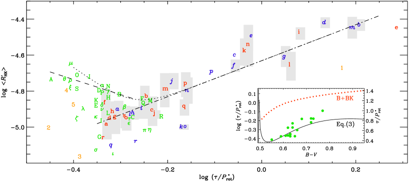
Figure 2.— Similar to Figure 1, but now with rotation periods computed from $B-V$ using Equation (2) and the assumption that M67 is $4\,{\rm Gyr}$ old. (The green symbols would end up further to the left if we assumed instead an age of $5\,{\rm Gyr}$.) Here all stars are included—not just those for which $P_{\rm rot}$ would also be available; see Table LABEL:TSum1. The inset shows $\tau/P_{\rm rot}^{\ast}$ as a function of $B-V$ using Equation (3). The data points for the stars of M67 are overplotted to illustrate the scatter and the range in $B-V$ covered by the data. The red dotted line without surrounding data points shows the result using the gyrochronology relation of Barnes (2010) and Barnes & Kim (2010) for $\tau(B-V)$, denoted by B+BK.

Next, we compare with the diagram where $\tau/P_{\rm rot}^{\ast}$ is estimated just from $B-V$ using gyrochronology; see Equation (2) and Figure 2. Now, the direct fit for the 15 stars with $\log\langle R^{\prime}_{\rm HK}\rangle\geq-4.85$ gives $\log c_{2}^{\rm dir}\approx-5.12$ and $\mu_{2}^{\rm dir}=-0.87$ and is shown as a dashed line. The inset reveals that $\tau/P_{\rm rot}^{\ast}$ is indeed a monotonically increasing function of $B-V$ in the range from $0.55$ to $0.8$, as asserted earlier in this section. The data points for the stars of M67 scatter around this line. The corresponding relation obtained using the gyrochronology relation of Barnes (2010) is also given. The difference of about $0.3$ dex results from the fact that the $\tau(B-V)$ of Barnes & Kim (2010) is nearly twice as large as that of Noyes et al. (1984).

As a function of $\tau/P_{\rm rot}^{\ast}$, the reversed trend of $\log\langle R^{\prime}_{\rm HK}\rangle$ is even more pronounced. S1420 (green S) appears now more rapidly rotating: $P_{\rm rot}^{\ast}=20.7\,{\rm d}$ whereas $P_{\rm rot}=24.8\,{\rm d}$; see Table LABEL:TSum1. Another example is S1106 (green L) where $P_{\rm rot}^{\ast}=24.3\,{\rm d}$ whereas $P_{\rm rot}=28.4\,{\rm d}$. On the other hand, S801 (green C), S1218 (green N), and S1307 (green R) are now predicted to rotate slower than what is measured. To understand these departures, we need to remind ourselves of the possibility of measurement errors, notably in $P_{\rm rot}$, variability of $\langle R^{\prime}_{\rm HK}\rangle$ associated with cyclic changes in their magnetic field, and of the intrinsically chaotic nature of stellar activity. Also, of course, the gyrochronology relation itself is only an approximation to empirical findings and not a physical law of nature.

3. Evolution and relation to reduced braking

Following van Saders et al. (2016) and Metcalfe & van Saders (2017), we would expect that evolved stars lose their large-scale magnetic field and thereby undergo reduced magnetic braking. Their angular velocity should then stay approximately constant until accelerated expansion occurs at the end of their main-sequence life. For those stars, it might be difficult or even impossible to ever enter the regime of antisolar DR. This could be the case for $\alpha$ Cen A (HD 128620, blue $k$), KIC 8006161 (blue $o$), and 16 Cyg A and B (HD 186408 and 186427, i.e., blue $q$ and $r$ symbols, respectively). These are stars that rotate faster than expected based on their extremely low chromospheric activity. Given the intrinsic variability of stellar magnetic fields, it is conceivable that the idea of reduced braking may not apply to all stars. Others would brake sufficiently to enter the regime of antisolar rotation and then exhibit enhanced activity, as discussed above. With increasing age, those stars would continue to slow down further and increase their chromospheric activity, as seen in Figure 2.

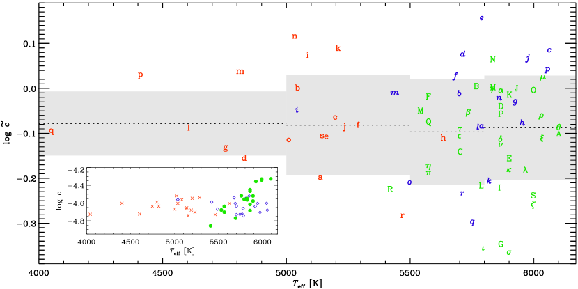
Figure 3.— Dependence of the residual $\log\tilde{c}$ on $T_{\rm eff}$, which corresponds to the dotted lines in Figures 1 and 2. Again, some of the symbols have been shifted to avoid overlapping. Average and standard deviation are computed for smaller $T_{\rm eff}$ intervals, as indicated by horizontal dotted lines and gray boxes, respectively. The inset shows the residual $\log c$ versus $T_{\rm eff}$.

It is in principle possible that stars with different $T_{\rm eff}$ show a systematic dependence of the residual

$$\log\tilde{c}=\log\langle R^{\prime}_{\rm HK}\rangle-\log\left[\;\mbox{``rhs of Equation~{}(\ref{representation})''}\;\right];$$ (7)

see the dotted lines in Figures 1 and 2. This is examined in Figure 3. It turns out that this residual is essentially flat, i.e., there is no systematic dependence on $T_{\rm eff}$, and it is consistent with random departures which do, however, becomes stronger toward larger $T_{\rm eff}$, as indicated by the gray boxes in Figure 3.

The work of Karak et al. (2015) has demonstrated that in the antisolar regime, the magnetic activity can indeed be chaotic and intermittent. Thus, depending on chance, a star in this regime may appear particularly active (e.g., S1252, green O symbol with $\log\langle R^{\prime}_{\rm HK}\rangle=-4.72$), while others could be particularly inactive (e.g., S969, green G symbol, with $\log\langle R^{\prime}_{\rm HK}\rangle=-5.06$). Other examples are S1449 (green $\sigma$ with $\log\langle R^{\prime}_{\rm HK}\rangle=-5.13$) and S1048 (green $\iota$ with $\log\langle R^{\prime}_{\rm HK}\rangle=-5.17$). We must therefore expect that the magnetic activity of some of these stars could still change significantly later in time, perhaps on decadal or multi-decadal timescales. In fact, we note from a comparison of the Ca ii measurements in Giampapa et al. (2017) with those from the initial chromospheric activity survey of over a decade ago (Giampapa et al., 2006) that the $R^{\prime}_{\rm HK}$ values for the specific stars mentioned above, S969 and S1048, are now each lower by about 20% while that for S1449 is lower by 23%.

Given that the more massive stars of M67 are on their way to becoming subgiants (e.g. Motta et al., 2016), we now discuss whether this could explain their enhanced activity. Properties important for convection such as luminosity and radius may increase substantially above the main sequence values before reaching the turnoff. To compare with observations, it is convenient to look at the usual residual $\log c=\log\langle R^{\prime}_{\rm HK}\rangle-\log(\tau/P_{\rm rot})$, which was given in the inset of Figure 1 as a function of $R^{\prime}_{\rm HK}$ and is now presented in the inset of Figure 3 as a function of $T_{\rm eff}$. We see that the four hottest stars of the sample, S603 (green A), S1095 (green J), S1252 (green O), and S1420 (green S) have a slight, but systematic excess. Assuming that their values of $R^{\prime}_{\rm HK}$ and $P_{\rm rot}$ are accurate, this could mean that the estimated values of $\tau$ are too small. Gilliland (1985) found that for a certain regime of evolution, stars of the solar mass and above may have $\tau$ significantly larger (up to $0.4\,{\rm dex}$) than those of main-sequence stars at the same effective temperature (see their Figure 10). However, the regime for this behavior occurred only when these stars cooled to below the solar main-sequence effective temperature. As can be seen in the color-magnitude diagram in Giampapa et al. (2006), our sample does not include stars which have cooled to this degree; on the contrary, our sample is still very near the main-sequence, and therefore we expect Equation (3) should still apply. This would therefore not alter our suggestion that most of the members of M67 have antisolar DR.

4. Conclusions

The phenomenon of antisolar DR is well known from theoretical models of solar/stellar convective dynamos in spherical shells. So far, antisolar DR has only been observed in some K giants (Strassmeier et al., 2003; Weber et al., 2005; Kővári et al., 2015, 2017) and subgiants (Harutyunyan et al., 2016), but not yet in dwarfs. Our work is compatible with the interpretation that the enhanced activity at large Rossby numbers (slow rotation) is a manifestation of antisolar DR. Our results are suggestive of a bifurcation into two groups of stars: those which undergo reduced braking and become inactive at $P_{\rm rot}/\tau\approx 2$ (van Saders et al., 2016), and those that enter the regime of antisolar rotation and continue to brake at enhanced activity, although with chaotic time variability. Interestingly, Katsova et al. (2018) have suggested that stars with antisolar DR may be prone to exhibiting superflares (Maehara et al., 2012; Candelaresi et al., 2014). This would indeed be consistent with the anticipated chaotic time variability of such stars.

The available time series are too short to detect antisolar DR through changes in the apparent rotation rate that would be associated with spots at different latitudes; see Reinhold & Arlt (2015) for details of a new technique. It is therefore important to use future opportunities, possibly still with Kepler, to repeat those measurements at later times when the magnetic activity belts might have changed in position.

References

- Baliunas et al. (1995) Baliunas, S. L., Donahue, R. A., Soon, W. H., Horne, J. H., Frazer, J., Woodard-Eklund, L., Bradford, M., Rao, L. M., Wilson, O. C., Zhang, Q., Bennett, W., Briggs, J., Carroll, S. M., Duncan, D. K., Figueroa, D., Lanning, H. H., Misch, T., Mueller, J., Noyes, R. W., Poppe, D., Porter, A. C., Robinson, C. R., Russell, J., Shelton, J. C., Soyumer, T., Vaughan, A. H., & Whitney, J. H. 1995, ApJ, 438, 269
- Barnes (2010) Barnes, S. A. 2010, ApJ, 722, 222
- Barnes & Kim (2010) Barnes, S. A., & Kim, Y.-C. 2010, ApJ, 721, 675
- Barnes et al. (2016) Barnes, S. A., Weingrill, J., Fritzewski, D., Strassmeier, K. G., & Platais, I. 2016, ApJ, 823, 16
- Brandenburg et al. (2017) Brandenburg, A., Mathur, S., & Metcalfe, T. S. 2017, ApJ, 845, 79 (BMM)
- Brown et al. (2011) Brown, B. P., Miesch, M. S., Browning, M. K., Brun, A. S., & Toomre, J. 2011, ApJ, 731, 69
- Candelaresi et al. (2014) Candelaresi, S., Hillier, A., Maehara, H., Brandenburg, A., & Shibata, K. 2014, ApJ, 792, 67
- Fan & Fang (2014) Fan, Y., & Fang, F. 2014, ApJ, 789, 35
- Gastine et al. (2014) Gastine, T., Yadav, R. K., Morin, J., Reiners, A., & Wicht, J. 2014, MNRAS, 438, L76
- Giampapa et al. (2017) Giampapa, M. S., Brandenburg, A., Cody, A. M., Skiff, B. A., & Hall, J. C. 2017, ApJ, submitted, http://www.nordita.org/preprints, no. 2017-121
- Giampapa et al. (2006) Giampapa, M. S., Hall, J. C., Radick, R. R., & Baliunas, S. L. 2006, ApJ, 651, 444
- Gilliland (1985) Gilliland, R. L. 1985, ApJ, 299, 286
- Gilman (1977) Gilman, P. A. 1977, Geophys. Astrophys. Fluid Dyn., 8, 93
- Harutyunyan et al. (2016) Harutyunyan, G., Strassmeier, K. G., Künstler, A., Carroll, T. A., & Weber, M. 2016, A&A, 592, A117
- Käpylä et al. (2014) Käpylä, P. J., Käpylä, M. J., & Brandenburg, A. 2014, A&A, 570, A43
- Karak et al. (2015) Karak, B. B., Käpylä, M. J., Käpylä, P. J., Brandenburg, A., Olspert, N., & Pelt, J. 2015, A&A, 576, A26
- Katsova et al. (2018) Katsova, M. M., Kitchatinov, L. L., Livshits, M. A., Moss, D. L., Sokoloff, D. D., & Usoskin, I. G. 2018, Astron. Rep., 95, 78
- Kővári et al. (2015) Kővári, Z., Kriskovics, L., Künstler, A., Carroll, T. A., Strassmeier, K. G., Vida, K., Oláh, K., Bartus, J., Weber, M. 2015, A&A, 573, A98
- Kővári et al. (2017) Kővári, Z., Strassmeier, K. G., Carroll, T. A., Oláh, K., Kriskovics, L., Kővári, E., Kovács, O., Vida, K., Granzer, T., & Weber, M. 2017, A&A, 606, A42
- Maehara et al. (2012) Maehara, H., Shibayama, T., Notsu, S., Notsu, Y., Nagao, T., Kusaba, S., Honda, S., Nogami, D., & Shibata, K. 2012, Nature, 485, 478
- Mamajek & Hillenbrand (2008) Mamajek, E. E., & Hillenbrand, L. A. 2008, ApJ, 687, 1264
- Metcalfe & van Saders (2017) Metcalfe, T. S., & van Saders, J. 2017, Solar Phys., 292, 126
- Motta et al. (2016) Motta, C. B., Salaris, M., Pasquali, A., & Grebel, E. K. 2016, MNRAS, 466, 2161
- Noyes et al. (1984) Noyes, R. W., Hartmann, L., Baliunas, S. L., Duncan, D. K., & Vaughan, A. H. 1984, ApJ, 279, 763
- Önehag et al. (2011) Önehag, A., Korn, A., Gustafsson, B., Stempels, E., & Vandenberg, D. A. 2011, A&A, 528, A85
- Reinhold & Arlt (2015) Reinhold, T., & Arlt, R. 2015, A&A, 576, A15
- Saar & Brandenburg (1999) Saar, S. H., & Brandenburg, A. 1999, ApJ, 524, 295 (SB)
- Sarajedini et al. (2009) Sarajedini, A., Dotter, A., & Kirkpatrick, A. 2009, ApJ, 698, 1872
- Strassmeier et al. (2003) Strassmeier, K. G., Kratzwald, L., & Weber, M. 2003, A&A, 408, 1103
- van Saders et al. (2016) van Saders, J. L., Ceillier, T., Metcalfe, T. S., Silva Aguirre, V., Pinsonneault, M. H., García, R. A., Mathur, S., & Davies, G. R. 2016, Nature, 529, 181
- Vilhu (1984) Vilhu, O. 1984, A&A, 133, 117
- Weber et al. (2005) Weber, M., Strassmeier, K. G., & Washuettl, A. 2005, Astron. Nachr., 326, 287