The Mount Wilson Observatory $S$-index of the Sun

Abstract

The most commonly used index of stellar magnetic activity is the instrumental flux scale of singly-ionized calcium H & K line core emission, $S$, developed by the Mount Wilson Observatory (MWO) HK Project, or the derivative index $R^{\prime}_{\rm HK}$. Accurately placing the Sun on the $S$ scale is important for comparing solar activity to that of the Sun-like stars. We present previously unpublished measurements of the reflected sunlight from the Moon using the second-generation MWO HK photometer during solar cycle 23 and determine cycle minimum $S_{\rm 23,min}=0.1634\pm 0.0008$, amplitude $\Delta S_{23}=0.0143\pm 0.0012$, and mean $\langle S_{23}\rangle=0.1701\pm 0.0005$. By establishing a proxy relationship with the closely related National Solar Observatory Sacramento Peak calcium K emission index, itself well-correlated with the Kodaikanal Observatory plage index, we extend the MWO $S$ time series to cover cycles 15–24 and find on average $\langle S_{\rm min}\rangle=0.1621\pm 0.0008$, $\langle\Delta S_{\rm cyc}\rangle=0.0145\pm 0.0012$, $\langle S_{\rm cyc}\rangle=0.1694\pm 0.0005$. Our measurements represent an improvement over previous estimates which relied on stellar measurements or solar proxies with non-overlapping time series. We find good agreement from these results with measurements by the Solar-Stellar Spectrograph at Lowell Observatory, an independently calibrated instrument, which gives us additional confidence that we have accurately placed the Sun on the $S$-index flux scale.

1. Introduction

Solar magnetic activity rises and falls in a roughly 11-year cycle that has been diligently measured with sunspot counts for over 400 years. Mechanical (i.e. magnetic) heating in chromospheric plage regions on the Sun leads to emission in the cores of the absorption lines Ca ii H & K (Linsky & Avrett, 1970; Athay, 1970). The correlation between HK emission and magnetic flux on the Sun (Skumanich et al., 1975; Harvey & White, 1999; Pevtsov et al., 2016), allows the study of magnetic variability on other stars, placing the Sun and its solar cycle in context. Olin Wilson’s HK Project at the Mount Wilson Observatory (MWO) regularly observed the Ca ii H & K emission for a sample of over 100 bright dwarf stars from early F to early M type beginning in 1966, for the first time characterizing long-term magnetic variability of stars other than the Sun (Wilson, 1978). A large body of work is derived from these observations which forms the basis of our understanding on the relationship between magnetic activity and variability on fundamental stellar properties (Hall, 2008). For example, Noyes et al. (1984) established that activity decreases with rotation rate and is influenced by stellar convection, with deeper convective zones resulting in higher activity. Sensitive differential photometry revealed the relationship between variation at visible wavelengths and magnetic activity, with the amplitude of photometric variability increasing with activity, as well as the separation of stars into high-activity spot-dominated and low-activity faculae-dominated photometric variability classes according to the sense of the correlation between visible photometry and activity (Lockwood et al., 1997; Radick et al., 1998; Lockwood et al., 2007). Using 25 years of MWO data, Baliunas et al. (1995) revealed the patterns of long-term magnetic variability in the Olin Wilson sample, finding cycling, flat, and irregularly variable stars. These results have been used to constrain and inform theoretical studies of solar and stellar dynamos, giving crucial information on the sensitivity of the dynamo to fundamental properties such as mass and rotation (Soon et al., 1993a; Baliunas et al., 1996; Saar & Brandenburg, 1999; Böhm-Vitense, 2007; Metcalfe et al., 2016).

Each of the above results places the Sun – the only star in which spatially resolved observations in a variety of bandpasses are available – in a stellar context. However, the usefulness of the solar-stellar comparison is only as good as the accuracy of the Sun’s placement on the stellar activity scale. The magnetic activity proxy established by the MWO HK project is the $S$-index:

$$S=\alpha\frac{N_{H}+N_{K}}{N_{R}+N_{V}}$$ (1)

where $N_{H}$ and $N_{K}$ are the counts in 1.09 Å triangular bands centered on Ca ii H & K in the HKP-2 spectrophotometer, and $N_{R}$ and $N_{V}$ are 20 Å reference bandpasses in the nearby continuum region, and $\alpha$ is a calibration constant (Vaughan et al., 1978).

The HKP-2 instrument is distinct from the coudé scanner used by Olin Wilson at the 100-inch telescope at MWO, later designated HKP-1 in Vaughan et al. (1978). HKP-1 was a two-channel photometer, with one 1 Å channel centered on either the H- or K-line and the other channel measuring two 25 Å bands separated by about 250 Å from the HK region (Wilson, 1968). HKP-1 measurements were therefore:

$$\begin{split}F_{H}&=\frac{N_{H}}{N_{\mathcal{R}}+N_{\mathcal{V}}}\\ F_{K}&=\frac{N_{K}}{N_{\mathcal{R}}+N_{\mathcal{V}}}\\ F&=\tfrac{1}{2}(F_{H}+F_{K})\end{split}$$ (2)

where we use $\mathcal{R}$ and $\mathcal{V}$ to distinguish the difference between the reference channels in the two instruments, with HKP-1 $\mathcal{R}$ and $\mathcal{V}$ being 5 Å wider than HKP-2 $R$ and $V$. The $\alpha$ parameter of equation (1) was determined nightly with the standard lamp and standard stars such that on average $S=F$ (Vaughan et al., 1978; Duncan et al., 1991). However, differences are expected given that the two instruments are not identical, and Vaughan et al. (1978) derived the following relation with coincident measurements on 13 nights in 1977:

$$F=0.033+0.9978\,S-0.2019\,S^{2}$$ (3)

It is important to stress that $S$ is an instrumental flux scale of the HKP-2 spectrophotometer that cannot be independently measured without cross-calibration using overlapping Mount Wilson targets. The consequence of this is that there are only two methods of placing the solar activity cycle on the $S$-index scale: directly measuring solar light with the HKP-2 instrument, or calibrating another measurement to the $S$-index scale using some proxy. Previously, only the latter method has been possible. In this work we analyze hitherto unpublished observations of the Moon with the HKP-2 instrument and determine the placement of the Sun on the $S$-index scale. We review past calibrations of solar $S$ in section 2. In section 3 we describe the observations used in the determination of solar $S$, and the analysis procedure in section 4. In section 5 we empirically explore the assertion that $S$ is linear with Ca K-line emission. We conclude in section 6 with a discussion on the implications of our results, and future directions for establishing the solar-stellar connection.

2. Previous Solar $S$ Proxies

Sun-as-a-star Ca ii H & K measurements have been made at Kitt Peak National Observatory (NSO/KP) on four consecutive days each month from 1974–2013 (White & Livingston, 1978), and at Sacramento Peak (NSO/SP) daily, albeit with with gaps, from 1976–2016. (Keil & Worden, 1984; Keil et al., 1998). Results from these observations for three solar cycles are given in Livingston et al. (2007). From the NSO/KP and NSO/SP spectrographs, the K emission index (hereafter $K$) is computed as the integrated flux in a 1 Å band centered on the Ca ii K-line normalized by a band in the line wing. The principal difference of $K$ with respect to $S$ is (1) $K$ includes flux only in the K line, while $S$ measures flux in both H and K, (2) the reference bandpass is in the line wing for $K$, as opposed to two 20 Å bands in the nearby pseudo-continuum region for $S$. These differences could be cause for concern relating $S$ to $K$, however (1) H and K are are a doublet of singly ionized calcium and thus are formed by the same population of excited ions, therefore the ratio $K/H$ cannot vary except by changes in the optical depth of the emitting plasma (Linsky & Avrett, 1970), which is unlikely to vary by a large amount (2) the far wing of the K line does vary somewhat over the solar cycle, however only to a level of 1% (White & Livingston, 1981). Therefore we can expect a priori that there should be a simple linear relationship between the $K$ and and $S$ indices. We investigate this assumption in detail in Section 5.

Table 1 $S(K)$ Transformations

Reference	$S(K)$	$S_{\rm 23,min}$	$S_{\rm 23,max}$	$\Delta S_{23}$	$\langle S_{23}\rangle$
Duncan et al. (1991)	$(1.58\pm 0.33)\,K+(0.040\pm 0.002)$ a	0.179	0.194	0.0151	0.187
White et al. (1992), original	$1.69\,K+0.016$ b	0.165	0.181	0.0162	0.173
White et al. (1992), mean	$(1.64\pm 0.07)\,K+(0.028\pm 0.007)$ b	0.172	0.188	0.0156	0.180
Baliunas et al. (1995)	$2.63\,K-0.066$ c	0.166	0.191	0.0251	0.178
Radick et al. (1998)	$(1.475\pm 0.070)\,K+(0.041\pm 0.013)$	0.171	0.185	0.0141	0.178
Hall & Lockwood (2004)	$1.359\,K+0.0423$ d	0.162	0.175	0.0130	0.168
This Work	$(1.50\pm 0.13)\,K+(0.031\pm 0.013)$	0.163	0.178	0.0143	0.170

Note. — ^a: Duncan’s $r_{\rm HK}$ replaced by $r_{\rm K}\equiv K$ using $r_{\rm HK}/r_{\rm K}=0.089/0.087$ from their paper. Uncertainties are from a formal linear regression done in White et al. (1992), who noted the slope uncertainty is unrealistically large. ^b: Original calibration used the NSO/KP measurements; this version is transformed to use the NSO/SP measurements using Equation 4 ^c: Calculated using the published intervals and $\langle S\rangle$ in Donahue & Keil (1995), along with the NSO/SP $K$ data. ^d: Calculated from the published yearly mean values of $S$ at cycle 23 minimum and maximum.

Several authors have developed transformations from the $K$ to MWO $S$-index, and the results are summarized in Table 1. The earliest attempt was from Duncan et al. (1991), who used spectrograms of 16 MWO stars taken between 1964 and 1966 at the coudé focus of the Lick 120 inch telescope to estimate a stellar $K$, and thereby establish a relationship with an average of $S$ for those stars from MWO. The Sun was also a data point used in determining the relationship, with its $K$ determined by NSO/KP and $S$ from Wilson (1978)’s observations of the Moon at cycle 20 maximum and cycle 20-21 minimum. Radick et al. (1998) revisited the Duncan et al. (1991) calibration using longer time averages of $S$ for the stars and $K$ for the Sun with updated observations, and adjusting the zero-point of the regression to force the Sun’s residual to zero. These approaches neglect the potential difference in scaling among the NSO/SP or NSO/KP $K$-indices and the $K$-index derived from the Lick Spectrograph, but such a cross correlation is not feasible in any case, due to the lack of common targets for the different spectrographs. Furthermore, this method only uses a single measurement of the $K$-index for the stellar sample, while the $S$-index is a decades-long average from Mount Wilson data. This poor sampling of $K$ will result in large scatter due to rotational and cycle-scale activity for the active stars in the sample, increasing the uncertainty in the determination of the $S(K)$ scaling relation.

White et al. (1992) took another approach, leveraging Olin Wilson’s observations of the Moon with the original HKP-1 instrument during cycle 20 (Wilson, 1978, Table 3). However, because the HKP-1 Moon observations did not overlap with the NSO $K$-index programs, those time series had to be projected back in time using an intermediary solar activity proxy, the 10.7 cm radio flux measurements (hereafter abbreviated $F_{10.7}$). White et al. (1992) was discouraged that the result from this method was discrepant with the Duncan et al. (1991) calibration, and citing the validity of both approaches, they chose to average the two results.

The White et al. (1992) $S(K)$ relationship was based on the NSO/KP data, which is on a slightly different flux scale than the NSO/SP data we use in this work. White et al. (1998) determined a linear relationship between the two instruments to be $K_{\rm KP}=1.1\,K_{\rm SP}-0.01$. Using a cycle shape model fit (see section 4.2), we determined the cycle minima preceding cycles 22, 23, and 24, and the maxima of cycles 21, 22, and 23 in both data sets. Then, using a ordinary least squares regression on these data, we obtained:

$$K_{\rm KP}=1.143\,K_{\rm SP}-0.0148$$ (4)

which is in agreement with the White et al. (1998) relationship to the precision provided. We substitute (4) in the White et al. (1992) original and mean transformations and the results are shown in Table 1. Note that in the mean with Duncan et al. (1991) transformation we do not use equation (4) in the latter, as it was determined from stellar observations using the Lick spectrograph, and therefore not specific to NSO/KP data.

Baliunas et al. (1995) observed that the White et al. (1992) result failed to cover the cycle 20-21 minima values of (Wilson, 1978, Table 3). Furthermore, they noted that their calibration resulted in maxima for cycles 21 and 22 that were approximately equal to the amplitude of cycle 20 measured by Wilson with HKP-1, while other activity proxies (the sunspot record and $F_{10.7}$) show cycle 20 to be significantly weaker than cycles 21 and 22. With these problems in mind, Baliunas et al. (1995) derived a new transformation $S(K)$ which smoothed the cycle 20 to 21 minima transition from the Wilson measurements to the $S(K)$ proxy and preserved the relative amplitudes found in $F_{10.7}$ and sunspot records. This transformation was not published, however it was used again in Donahue & Keil (1995) who published mean $S$ values from this transformation for several intervals. Using these intervals and mean values along with the NSO/SP record we computed the Baliunas et al. (1995) $S(K)$ relationship, which is shown in Table 1.

The Solar-Stellar Spectrograph (SSS) at Lowell Observatory synoptically observes the Ca H & K lines for $\sim$100 FGK stars, as well as the Sun (Hall & Lockwood, 1995; Hall et al., 2007). The spectra are placed on an absolute flux scale, and the MWO $S$-index is determined using an empirically calibrated relationship (Hall & Lockwood, 1995). The calibration is shown to be consistent with actual MWO observations to a level of 7% rms for low-activity stars (see Figure 4 Hall et al., 2007). In Hall & Lockwood (2004), mean values of $S$ for cycle 23 minimum and maximum were published, which we used with the NSO/SP data to derive an $S(K)$ transformation, shown in Table 1. Hall & Lockwood (2004) remarked that their cycle 23 $S$ amplitude was “noticeably less” than the Baliunas et al. (1995) amplitude for the stronger cycle 22 (as evidenced from other proxies, such as the sunspot record). Subsequent re-reductions of the SSS solar time series in Hall et al. (2007) and Hall et al. (2009) reported mean values of 0.170 and 0.171 for cycle 23 observations, $\sim 5$% lower than the mean value of 0.179 reported in Baliunas et al. (1995) for cycles 20–22.

We used the cycle shape model fit (see section 4) to determine the values of the cycle 22-23 minima and cycle 23 maxima in the NSO/SP $K$ timeseries. We also computed the mean value $\langle K\rangle$ of cycle 23 from this data set. The conversion of these $K$ values to $S$ using the previously published relationships is shown in Table 1. Each relationship arrives at different conclusions about the placement of solar minimum, maximum, and mean value for this cycle. The relative range (max - min)/mean of minima positions is $\approx$ 10%, amplitudes $\approx$ 81%, and cycle means $\approx$ 11%. These discrepancies are significantly larger than the uncertainty of the determination of these values from $K$, which we estimate has an daily measurement uncertainty of $\sim$ 1% (see Section 4) and a cycle amplitude of 6% above minimum. The largest discrepancy, as Hall & Lockwood (2004) noted, is in the cycle amplitude, with the Baliunas et al. (1995) $S(K)$ proxy estimate being more than double their measurement. Considering the variety and magnitude of these discrepancies, we conclude that the solar $S$-index has so far not been well understood.

3. Observations

3.1. Mount Wilson Observatory HKP-1 and HKP-2

The Mount Wilson HK Program observed the Moon with both the HKP-1 and HKP-2 instruments. After removing 11 obvious outliers there are 162 HKP-1 observations taken from 2 Sep 1966 to 4 Jun 1977 with the Mount Wilson 100-inch reflector, covering the maximum of cycle 20 and the cycle 20-21 minimum. Wilson (1968) and Duncan et al. (1991) published mean values from these data, with the latter shifted upward by about 0.003 in $S$. Our HKP-1 data is under the same calibration as in Duncan et al. (1991) and Baliunas et al. (1995).

As mentioned in Baliunas et al. (1995), observations of the Moon resumed in 1993 with the HKP-2 instrument. After removing 10 obvious outliers there are 75 HKP-2 observations taken from 27 Mar 1994 to 23 Nov 2002 with the Mount Wilson 60-inch reflector, covering the end of cycle 22 and the cycle 23 minimum, extending just past the cycle 23 maximum. The end of observations coincides with the unfortunate termination of the HK Project in 2003. These observations were calibrated in the same way as the stellar HKP-2 observations as described in Baliunas et al. (1995), using the standard lamp and measurements from the standard stars. Long-term precision of the HKP-2 instrument was shown to be 1.2% using 25 years of observations in a sample of 13 stable standard stars.

The 75 HKP-2 lunar observations are the only observations of solar light with the HKP-2 instrument, and thus are the only means of directly placing the Sun on the instrumental $S$-index scale of equation (1). We assume that these observations measure $S$ for the Sun to within the 1.2% precision determined for the HKP-2 instrument. Most HKP-1 and HKP-2 observations were taken within 5 days of full Moon, and all observations were taken within an hour of local midnight. We do not expect a significant alteration of the nearby spectral bands constituting $S$ by reflection from the Moon, which is to first order a gray diffuse reflector.

3.2. NSO Sacramento Peak K-line Program

We seek to extend our time series of solar variability beyond cycle 23 by establishing a proxy to the NSO Sacramento Peak (NSO/SP) observations taken from 1976–2016, covering cycles 21 to 24. The NSO/SP K-line apparatus is described in Keil & Worden (1984). Briefly, it consists of a $R\sim 150,000$ Littrow spectrograph installed at the John W. Evans Solar Facility (ESF) at Sacramento Peak Observatory, fed by a cylindrical objective lens which blurs the Sun into a 50 $\mu$m by 10 mm line image at the spectrograph slit. The spectral intensity scale is set by a integrating a 0.53 Å band centered at 3934.869 Å in the K-line wing and setting it to the fixed value of 0.162. The $K$ emission index is then defined as the integrated flux of a 1 Å band centered at the K-line core (3935.662 Å) (White & Livingston, 1978). We estimated the measurement uncertainty to be 1.0% by calculating the standard deviation during the period 2008.30–2009.95, which is exceptionally flat in the sunspot record and 10.7 cm radio flux time series.

3.3. Kodaikanal Observatory Ca K Spectroheliograms

We extend the $S$-index record back to cycle 20 using the composite $K$ time series of Bertello et al. (2016), which is available online (Pevtsov, 2016). This composite calibrates the NSO/SP data to K-line observations by the successor program at NSO, the Synoptic Optical Long-term Investigations of the Sun (SOLIS) Integrated Sunlight Spectrometer (ISS) (Bertello et al., 2011). The calibration used in Bertello et al. (2016) is:

$$K_{\rm ISS}=0.8781\,K_{\rm SP}+0.0062$$ (5)

Bertello et al. (2016) calibrated the synoptic Ca ii K plage index from spectroheliograms from the Kodaikanal (KKL) Observatory in India to the ISS flux scale using the overlapping portion NSO/SP data, resulting in a time series of Ca ii K emission from 1907 to the present. We transform this composite timeseries from the ISS flux scale to the NSO/SP flux scale by applying the inverse of equation (5):

$$K_{\rm KKL(SP)}=1.1388\,K_{\rm KKL(ISS)}-0.0071$$ (6)

We prefer this homogeneous chromospheric K-line proxy (hereafter denoted simply $K_{\rm KKL}$) over proxies based on photospheric phenomena such as $F_{10.7}$ or the sunspot number. In particular, Pevtsov et al. (2014) found that the correlation between $K$ and $F_{10.7}$ is non-linear and varies with the phase of the solar cycle, with strong correlation during the rising and declining phases, and poor correlation at maximum and minimum, precisely the sections of the solar cycle of most interest in this work.

3.4. Lowell Observatory Solar Stellar Spectrograph: Updated Data Reduction

We compare our results to a new reduction of observations from the Lowell Observatory Solar-Stellar Spectrograph (SSS), which is running a long-term stellar activity survey complementary to the MWO HK Project. The SSS observes solar and stellar light with the same spectrograph, with the solar telescope consisting of an exposed optical fiber that observes the Sun as an unresolved source (Hall & Lockwood, 1995; Hall et al., 2007). The basic measurement of SSS is the integrated flux in 1 Å bandpasses centered on the Ca ii H & K cores from continuum-normalized spectra, $\phi_{\rm HK}$, which can then be transformed to the $S$-index using a combination of empirical relationships derived from stellar observations:

$$S_{\rm SSS}=\frac{10^{14}\mathcal{F}_{\rm c,\lambda 3950}}{K_{\mathcal{F}}C_{\rm cf}T_{\rm eff}^{4}}\phi_{\rm HK}$$ (7)

where $\mathcal{F}_{\rm c,\lambda 3950}$ is the continuum flux scale for the Ca ii H & K wavelength region, which converts $\phi_{\rm HK}$ to physical flux (erg cm^-2 s^-1). $\mathcal{F}_{\rm c,\lambda 3950}$ is a function of Strömgren $(b-y)$ and is taken from Hall (1996). $K_{\mathcal{F}}$ (simply $K$ in other works) is the conversion factor between the MWO HKP-2 H & K flux (numerator of equation (1)) to physical flux (Rutten, 1984). $C_{\rm cf}$ a factor that removes the color term from $S$, and is a function of Johnson $(B-V)$ (Rutten, 1984). Finally, $T_{\rm eff}$ is the effective temperature. See Hall et al. (2007) and Hall & Lockwood (1995) for a details on the extensive work leading to this formulation. What is important to realize about this method of obtaining $S$ is that it requires three measurements of solar properties, $(b-y)_{\sun}$, $(B-V)_{\sun}$, and $T_{\rm eff,\sun}$, along with the determination of one constant, $K_{\mathcal{F}}$. The solar properties are taken from best estimates in the literature, which vary widely depending on the source used, and can dramatically affect the resulting $S_{\rm SSS}$ for the Sun. Hall et al. (2007) used $(b-y)_{\sun}=0.409$, $(B-V)_{\sun}=0.642$, and $T_{\rm eff,\sun}=5780$ K. The constant $K_{\mathcal{F}}$ was empirically determined to be $0.97\pm 0.11$ erg cm^-2 s^-1 in Hall et al. (2007) as the value which provides the best agreement between $S_{\rm SSS}$ and $S_{\rm MWO}$ from Baliunas et al. (1995) for an ensemble of stars and the Sun. This combination of parameters resulted in a mean $S_{\rm SSS}$ of 0.170 for the Sun using observations covering cycle 23. A slightly different calibration of SSS data in Hall & Lockwood (2004) used a flux scale $\mathcal{F}_{\rm c,\lambda 3950}$ based on Johnson $(B-V)$, set to 0.65 for the Sun, and $T_{\rm eff,\sun}=5780$ K. In Table 1 we estimated that this calibration resulted in a mean $S=0.168$ for cycle 23. Hall et al. (2009), which included a revised reduction procedure and one year of data with the upgraded camera (see below), found $\langle S\rangle=0.171$.

As mentioned previously, the three solar properties $(b-y)_{\sun}$, $(B-V)_{\sun}$, and $T_{\rm eff,\sun}$ used in the SSS flux-to-$S$ conversion are not accurately known. The fundamental problem is that instruments designed to observe stars typically cannot observe the Sun. Cayrel de Strobel (1996) studied this problem, and collected $(B-V)_{\sun}$ from the literature ranging from 0.62 to 0.69. Meléndez et al. (2010) compiled literature values $(b-y)_{\sun}$ ranging from 0.394 to 0.425. $T_{\rm eff,\sun}$ is more accurately known, which is fortunate given that it appears in equation (7) to the fourth power. However, a 0.01 change in $(B-V)_{\sun}$ or $(b-y)_{\sun}$ results in an approximately 2% or 10% change in $S_{\rm SSS}$, respectively. The sensitivity of $S_{\rm SSS}$ to these properties makes it especially important to use the best known values.

More recent photometric surveys of solar analogs have resulted in improved determinations of the solar properties by way of color-temperature relations. We are therefore motivated to update $S_{\rm SSS}$ for the Sun using these measurements: $(B-V)_{\sun}=0.653\pm 0.003$ (Ramírez et al., 2012), $(b-y)_{\sun}=0.4105\pm 0.0015$ (Meléndez et al., 2010), and $T_{\rm eff,\sun}=5772.0\pm 0.8$ (IAU General Assembly 2015 Resolution B3). The latter lower value for the effective temperature follows from the recent lower estimate of total solar irradiance in Kopp & Lean (2011). The constant $K_{\mathcal{F}}$ is kept at 0.97 as determined in Hall et al. (2007). The SSS data analyzed here now include data taken after upgrading the instrument CCD to an Andor iDus in early 2008 (Hall et al., 2009). This new CCD has higher sensitivity in the blue and reduced read noise. The reduction procedure remains the same as described in Hall et al. (2007) and on the SSS web site, albeit with updated software and two additional steps: (1) high S/N spectra from the new camera are used as reference spectra for the old camera data, which improves stability of the older data and avoids discontinuity at the camera upgrade boundary (2) an additional scaling correction is applied to the continuum-normalized spectra so that the line wings are shifted to match the normalized intensity of the Kurucz et al. (1984) solar spectrum. Despite these efforts, a non-negligible discontinuity was apparent across the CCD upgrade boundary. We suspect this may be due to minute differences in CCD pixel size, and the slightly different wavelength sampling at the continuum normalization reference points. The discontinuity is corrected post facto by multiplying the CCD-1 $S$ data by 0.9710, determined by the ratio of the medians for the last year of CCD-1 data to the first year of CCD-2 data. Finally, due to tape degradation, raw CCD data from 1998-2000 were lost, preventing reduction using the updated routines. Continuum normalized spectra from that period still exist, though introducing them into the updated pipeline results in significant discontinuities in $S$ which had to be corrected. The correction consisted of applying an additional scaling factor to the lost data region such that the region median falls on a linear interpolation of the cycle across the region. Keeping or removing the “corrected” data in this region does not affect our conclusions. Finally, we estimated the measurement uncertainty to be 1.6% for CCD-1, and 1.3% for CCD-2, by computing the standard deviation of observations from each device in the long minimum from 2007–2010.

4. Analysis

Our goal in this work is to use the 75 HKP-2 observations to determine the $S$-index for the Sun. Specifically, we seek to measure the minimum, maximum, and mean value of $S$ over several solar cycles. We proceed first by directly measuring these quantities using our cycle 23 HKP-2 data, and then establish a proxy with the NSO/SP measurements to extend our measurements to other cycles.

4.1. Cycle 23 Direct Measurements

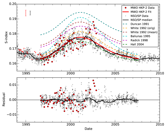
Figure 1.— Cycle 23 data and cycle shape model fits. The MWO HKP-2 Moon observations are shown in red, with the larger points used in the cycle shape model fit, which is shown as a thick red curve. NSO/SP $K$-index data are transformed to the $S$ scale using equation (12). A 1-yr wide median filter applied to the NSO/SP data is shown in the solid black line. $S(K)$ transformations of found in the literature (see Table 1) of a cycle shape model fit to the NSO/SP $K$ data are shown as colored curves for comparison. The bottom panel shows the residual difference of the cycle shape model curve and the data. Error bars in the top left show the estimated measurement uncertainty for MWO HKP-2 (red) and NSO/SP (black).

The HKP-2 data can be used to measure the minimum, maximum and mean of cycle 23 directly, but first the time of minimum and maximum must be established by some other means. We choose to use the NSO/SP $K$ record for this purpose. Applying a 1-yr boxcar median filter to the NSO/SP time series, we find the absolute minimum between cycles 22-23 at decimal year 1996.646, and absolute maximum at 2001.708. In this interval defining cycle 23, there are 56 HKP-2 measurements, with the remaining 19 points belonging to cycle 22. Next, using the HKP-2 time series, we take the median of a 2-yr wide window centered at the minima and maxima times to find $S_{\rm 23,min}=0.1643$ ($N=17$) and $S_{\rm 23,max}=0.1755$ ($N=12$), for a cycle 23 amplitude $\Delta S_{23}=0.0112$. The mean value for the cycle $\langle S_{23}\rangle=0.172$ (N = 56). We choose the median over the mean when measuring fractions of a cycle because we do not expect Gaussian distributions in that case. We choose a 2-yr wide window to be about as wide as we can reasonably go without picking up another phase of the solar cycle. Still, the number of points in each window is low, which does not give much confidence that the cycle can be precisely measured in this way. We shall investigate the uncertainty of this method in the next section. For the cycle mean, besides the problem of low sampling, we would expect this to be an overestimate since no data exists for the longer declining phase of the cycle.

Nonetheless, even with these simple estimates we find discrepancies with the previous work shown in Table 1. The measured minimum is appreciably lower than the Duncan et al. (1991), White et al. (1992) mean, and Radick et al. (1998) values, and the amplitude is lower than all other estimates. Our cycle mean is also lower than all but the Hall & Lockwood (2004) estimate, indicating that the previous work has overestimated the $S$-index of the Sun. In the next section we will attempt to improve our precision using a method in which more of the data are used.

4.2. Cycle Shape Model Fit for Cycle 23

Due to the limited data we have from HKP-2 for cycle 23, the results of the previous section are susceptible to appreciable uncertainties from unsampled short-timescale variability due to rotation and active region growth and decay. By fitting a cycle model to our data, we can reduce the uncertainty in our minimum and maximum point determinations. We use the skewed Gaussian cycle shape model of Du (2011) for this purpose:

$$f(t)=A\exp\left(-\frac{(t-t_{m})^{2}}{2B^{2}\left[1+\alpha(t-t_{m})\right]^{2}}\right)+f_{\rm min}$$ (8)

where $t$ is the time, $A$ is the cycle amplitude, $t_{m}$ is approximately the time of maximum, $B$ is roughly the width of the cycle rising phase, and $\alpha$ is an asymmetry parameter. $f_{\rm min}$, which was not present in the Du model, is an offset which sets the value of cycle minimum. We also tried the quasi-Planck function of Hathaway et al. (1994) for this purpose and obtained similar results, however we prefer the above function due to the simplicity of interpreting its parameters and developing heuristics to guide the fit. We fit the model to the data using the Python scipy library curve_fit routine with bounds. This function uses a Trusted Region Reflective (TRR) method with the Levenberg-Marquardt (LM) algorithm applied to trusted-region subproblems (Branch et al., 1999; Moré, 1978). The fitting algorithm searches for the optimum parameters from a bounded space within $\pm 50$% of heuristic values obtained using a 1-yr median filter of the data, with the exception of $f_{\rm min}$ which has a lower bound set at the lowest data point in order to prevent the fitting procedure from underestimating the minimum.

The 56 HKP-2 data points contained in cycle 23 only cover the rising phase and are not enough to constrain a least-squares fitting procedure. To circumvent this problem, we first fit the NSO/SP data and assume that the parameters which determine the cycle shape $t_{m}$, $B$, and $\alpha$ are the same in the two chromospheric time series. The only way this assumption could fail is if the Ca ii H band, or the 20 Å continuum bands of $S$ (equation 1) varied in such a way as to distort the cycle shape with respect to $K$. Soon et al. (1993b) explored the long-term variability of the $C_{\rm RV}$ index based on the 20 Å reference bands, finding it to be generally quite small. We therefore assume for the moment that the H, R, and V bands are linear with $K$ or constant, and later confirm these assumptions in Section 5. Fitting equation (8) to the NSO/SP $K$ for cycle 23, we find $t_{m}=2001.122$, $B=2.154$, and $\alpha=0.0343$. We then hold these parameters fixed and fit equation (8) to the 56 HKP-2 observations for cycle 23, finding the remaining free parameters $A=0.0150,f_{\rm min}=0.163$.

The cycle model fit and the HKP-2 data are shown as the red curve in Figure 1. The reduced $\chi^{2}$ of the fit is 6.45, which we find acceptable given the model does not seek to explain all the variation in the data (e.g. rotation, active region growth and decay), only the mean cycle. We find an RMS residual of the fit of $\sigma_{\rm res}=0.0047$, which is a bit more than double the estimated individual measurement uncertainty $\sigma=0.0020$.

Using the cycle model fit, we find the minimum $S_{\rm 23,min}=0.1634\pm 0.0008$, maximum $S_{\rm 23,max}=0.1777\pm 0.0010$, and amplitude $\Delta S_{23}=0.0143\pm 0.0012$. The mean of the cycle model curve is $\langle S_{23}\rangle=0.1701\pm 0.0005$. The uncertainties are determined from a Monte Carlo experiment in which we build a distribution of cycle model fits from only 56 points of NSO/SP $K$ data during the rising phase of cycle 23, and comparing that to the “true” cycle model fit using all 1087 observations throughout the cycle (see Appendix A for details). The Monte Carlo experiment shows that the cycle model fit method with only 56 randomly selected points finds true minima and maxima with a $1\sigma$ standard deviation of $\approx$0.5%, while the method of direct means finds minima equally well, but maxima with about double the uncertainty due to the increased variability at that phase of the cycle.

Our results for cycle 23 are shown in the final row of Table 1, and are discrepant with most of the previous literature values. Hall & Lockwood (2004) comes closest to our result, though their amplitude is 9% lower. The Radick et al. (1998) amplitude is only 0.002 $S$-units (1.4%) lower than ours, but the mean is 4.7% higher due to the higher value for solar minimum. The Baliunas et al. (1995) relation finds a minimum only 1.8% higher than ours, but the amplitude is substantially larger (75%), leading to a 4.7% higher estimate of the solar cycle mean.

The cycle shape model fit to the NSO/SP $K$ data is transformed using the literature relations in Table 1 and are shown as colored curves in Figure 1. Here we see that no transformation matches the MWO HKP-2 observations in a satisfactory way, though the Hall & Lockwood (2004) curve comes close. In the next section we will construct a new $S(K)$ transformation that exactly matches our cycle shape model curve in Figure 1.

4.3. $S(K)$ Proxy Using NSO/SP $K$ Emission Index

We now seek a transformation between the NSO/SP $K$ emission index and the Mount Wilson $S$-index. We assume a linear relationship:

$$S(K)=a+b\,K$$ (9)

Now we write $K$ as a function of time using the cycle shape model (equation 8), obtaining:

$$S(t)=(a+bf_{{\rm min},K})+bA_{K}\,E(t;t_{m},B,\alpha)$$ (10)

where $E(t;t_{m},B,\alpha)$ is the exponential function from (8). This is precisely the same form as (8), which is made more clear by defining $f_{{\rm min},S}=(a+bf_{{\rm min},K})$ and $A_{S}=bA_{K}$. These definitions may be used as the solutions for $\{a,b\}$ when cycle shape model fits have been done for both $K(t)$ and $S(t)$, as was done in the previous section, giving

$$\begin{split}a&=f_{{\rm min},S}-(A_{S}/A_{K})\,f_{{\rm min},K}\\ b&=A_{S}/A_{K}.\end{split}$$ (11)

Note that the cycle shape parameters $\{t_{m},B,\alpha\}$ are not explicitly related to $\{a,b\}$. Using the cycle 23 fit parameters described in the previous section, we arrive at the following linear transformation:

$$S(K)=(1.50\pm 0.13)K+(0.031\pm 0.013)$$ (12)

The uncertainty in the slope and intercept are calculated using standard error propagation methods on equation (11).

$$\begin{split}\sigma_{b}^{2}&=b^{2}\,((\sigma_{A_{S}}/A_{S})^{2}+(\sigma_{A_{K}}/A_{K})^{2})\\ \sigma_{f_{K}\cdot b}^{2}&=(f_{K}\cdot b)^{2}\cdot[(\sigma_{b}/b)^{2}\\ &+(\sigma_{f_{K}}/f_{K})^{2}+2\,(\sigma_{b}/b)\,(\sigma_{f_{K}}/f_{K})\,\rho(f_{K},b)]\\ \sigma_{a}^{2}&=\sigma_{f_{S}}^{2}+\sigma_{f_{K}\cdot b}^{2}-2\,\sigma_{f_{S}}\,\sigma_{f_{K}\cdot b}\,\rho(f_{S},f_{K}\cdot b)\end{split}$$ (13)

where we have simplified the notation with $f_{K}\equiv f_{{\rm min},K}$ and $f_{S}\equiv f_{{\rm min},S}$. Correlation coefficients $\rho(x,y)$ for quantities $x$ and $y$ are defined as $\rho(x,y)={\rm cov}(x,y)/(\sigma_{x}\cdot\sigma_{y})$. We approximate $\rho(f_{K},b)\sim\rho(f_{K},A_{K})$ and $\rho(f_{S},f_{K\cdot b})\sim\rho(f_{S},A_{S})$, which likely overestimates the correlation between these quantities. The uncertainties of each of the curve fit parameters are obtained from Monte Carlo experiments described in Appendix A. Correlation between $A_{S}$ and $A_{K}$ through the cycle shape parameters $\{t_{m},B,\alpha\}$ is included in our estimate of $\sigma_{A_{S}}$ due to the setup of the Monte Carlo experiment (see Appendix A). The error budget is dominated by $(\sigma_{A_{S}}/A_{S})^{2}$, $(\sigma_{b}/b)^{2}$, and $\sigma_{f_{S}}^{2}$, with all other terms accounting for less than 5% of the total in their respective equations.

The estimated uncertainty of the cycle shape model cross-calibration method described above is significantly less than was achieved by linear regression of coincident measurements. The latter method had formal uncertainties in the scale factor in excess of 100%. Linear regression failed because we have few coincident measurements and the individual measurement uncertainty of $\approx$ 1% in both $K$ and $S$ is roughly 10% the amplitude of the variability over the cycle.

We transformed the NSO/SP $K$-index time series using equation (12) and plotted it with the MWO HKP-2 data and cycle shape model fits in Figure 1. A 1-yr boxcar median filter of the data is also plotted as a black line, which is in good agreement with the cycle shape model curve.

4.4. Comparison with SSS Solar Data

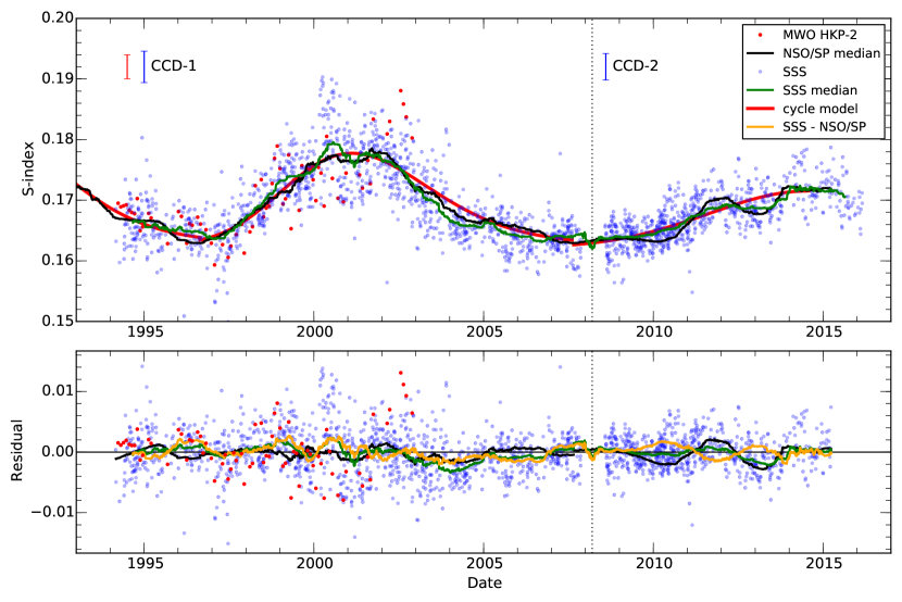
Figure 2.— SSS solar observations (blue) compared to the MWO HKP-2 measurements (red) and the NSO/SP $S(K)$ proxy, shown here as a running 1-yr median (black). Cycle shape model curves fit to the NSO/SP data are shown in red. The vertical dotted line denotes the upgrade of the SSS CCD. The bottom panel shows the residual difference of the data with the cycle shape model, while the orange line is the difference between the SSS (green) and NSO/SP (black) running medians. Error bars in the top panel show the estimated measurement uncertainty for SSS CCD-1 and CCD-2 observations (blue), and MWO HKP-2(red).

As an additional check of our transformation of the NSO/SP data to the $S$-index scale, we compare our result to the independently calibrated Solar-Stellar Spectrograph (SSS) observations described in section 3.4.

In Figure 2 we overplot the Lowell Observatory SSS solar $S$-index data on our NSO/SP $S(K)$ proxy for cycles 22, 23 and 24. A 1-yr median filter line is plotted for both time series, as well as the cycle shape model curves fit to the NSO/SP $S(K)$ data using the TRR+LM algorithm described in section 4.2. In general, we find excellent agreement between all three curves. We use the cycle shape model curves as a reference to compare the NSO/SP $S(K)$ proxy with SSS. For cycle 23, which is covered by the SSS CCD-1 data, the mean of the residual is -0.00031 $S$-units with a standard deviation of 0.0040 $S$. This may be compared to the NSO/SP data for the same period used to constrain the model fit, with an essentially zero mean and a standard deviation of 0.0032 $S$. Similarly for cycle 24, SSS CCD-2 data have a residual mean of -0.000097 $S$ and standard deviation of 0.0026, compared to the NSO/SP residual mean of -0.000047 $S$ and standard deviation 0.0028 $S$. In the case of cycle 24, SSS observations have a lower residual with the cycle model than the NSO/SP data used to define it! The difference of the SSS and NSO/SP running medians is shown as an orange line in Figure 2, and rarely exceeds $\pm 0.002$ $S$.

We now consider whether the remarkable agreement is confirmation of the true solar $S$-index, or mere coincidence. As discussed in section 3.4, the computation of $S$ from SSS spectra is sensitive to the measurement of solar color indices and the effective temperature. We have recalibrated the data with the best available measurements of these quantities. The resulting calibration results in a 3% scaling difference between CCD-1 and CCD-2 data, which we choose to remove by rescaling CCD-1 data to the CCD-2 scale, which resulted in the excellent agreement with NSO/SP $S(K)$. There is good reason for this choice, since CCD-2 is a higher quality detector. However, if there were a significant offset between the NSO/SP $S(K)$ and SSS, we would be justified in applying a small scaling factor to reconcile differences, citing uncertainties in the solar properties or the conversion factor $K_{\mathcal{F}}$. The fact that this was not necessary might be considered coincidence. However, the fact that only a scaling factor would be required, and not an absolute offset, can not be coincidence. From our determination of the $S(K)$ scaling relation (12) using equation (11), we see that using a different amplitude $A_{S}$ would change the scale of the conversion, $b$, and the offset, $a$, which could not be confirmed by these SSS data using a scaling factor alone. Therefore, the agreement between SSS and the NSO/SP $S(K)$ proxy can be taken as confirmation of the latter. The agreement between SSS and the MWO HKP-2 data points (red points in Figure 2) is confirmation that $S_{\rm SSS}$ is properly calibrated for the Sun.

4.5. Calibrating HKP-1 Measurements

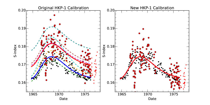
Figure 3.— Cycle 20 data and cycle shape model fits. Left: The original HKP-1 data are plotted as red circles, with a cycle shape model fit to those data as a red line. Monthly averaged $K_{\rm KKL}$ data transformed to the $S$-index scale using equation (12) are shown as black points, and a cycle shape model fit to those data as a blue line. Transformations of the $K_{\rm KKL}$ curve to $S$ using relationships found in the literature (see Table 1) are shown as colored curves for comparison, using the same color scheme as in Figure 1. Right: HKP-1 data calibrated to the HKP-2 scale using equation (14)

A simple inspection of the HKP-1 data alongside the HKP-2 data reveals that the calibration of HKP-1 data to the HKP-2 $S$-index scale could be improved. Notably, the HKP-1 data appear higher than the HKP-2 data. Here we perform a simple analysis analogous to that of section 4.1 to illustrate the problem. Using the cycle boundaries and times of maxima of Hathaway et al. (1999) based on the sunspot record, we take the cycle 20 maximum to be 1969/03 and the cycle 20-21 minimum to be 1976/03. We compute the median of a 2-yr window of the MWO HKP-1 data at these points giving $S_{\rm 20,max}=0.182$ (N=35), and $S_{\rm 21,min}=0.168$ (N=54). Taking the difference we find $\Delta S_{20}=0.014$.

The amplitude $\Delta S_{20}$ is slightly less than that of cycle 23, which agrees with the relative amplitudes of other activity proxies such as sunspot number and $F_{10.7}$ (Hathaway, 2015). However, the directly measured minima is 0.005 $S$-units higher than the cycle 23 value computed in the same way (Section 4.1) or with the cycle shape model fit (Section 4.2). This discrepancy, while small in an absolute sense, is over 1/3 of the cycle amplitude.

The discrepancy in the minima is not unexpected when one considers the uncertainties involved in calibrating the HKP-1 and HKP-2 instruments. They were calibrated using near-coincident observations for a sample of stars resulting in equation (3), but with individual stellar ($F$, $S$) means scattered about the calibration curve. Figure 5 of Vaughan et al. (1978) shows the calibration data and regression curve for HKP-1 $F$ and HKP-2 $S$. Near the solar mean $S$ of $\sim$0.170, scatter about the calibration curve of $\sim$5% is apparent. As a result, for any given star (or the Moon), an additional correction that in a shift of the mean of about $\sim$5% may be required to achieve continuity in the time series.

We apply such a correction to the HKP-1 Moon data to place it on the same scale as HKP-2. We use the $K_{\rm KKL}$ data as a proxy to tie the two datasets together, following a similar procedure described in Section 4.2.

First, we define the boundaries of cycle 20 as 1964/10 to 1976/03 as in Hathaway et al. (1999). We then fit a cycle shape model curve to the $K_{\rm KKL}$ data in this interval, obtaining the parameters $\{A_{\rm KKL},t_{m},B,\alpha,f_{{\rm min},{\rm KKL}}\}$. Holding the shape parameters $\{t_{m},B,\alpha\}$ fixed, we fit another curve to the HKP-1 data to find $\{A_{1},f_{{\rm min},1}\}$. Transforming the $K_{\rm KKL}$ curve amplitude and offset parameters $\{A_{\rm KKL},f_{{\rm min},{\rm KKL}}\}$ to the HKP-2 scale with equation (12), we obtain the HKP-2 parameters $\{A_{2},f_{{\rm min},2}\}$. Finally, using the analog of equation (11) for the HKP-1 and HKP-2 amplitude and offset parameters, we then obtain the transformation:

$$S_{\rm HKP-2}=0.9738\,S_{\rm HKP-1}-0.0025$$ (14)

Figure 3 shows the results of this new calibration. The left panel shows the HKP-1 data with the original calibration. Comparing the red curve (cycle shape model fit to the HKP-1 data) and the blue curve (fit to the $S(K_{\rm KKL})$ data with equation (12)), we see clearly the $\sim$$0.007\,S$ offset with the HKP-2 scale determined above. Literature relationships from Table 1 are also shown, as applied to a $K_{\rm KKL}$ cycle shape model curve. Agreement here is generally better than to the HKP-2 data, especially in the case of the Radick et al. (1998) calibration. Applying the HKP-1 to HKP-2 transformation of (14) to the MWO data, the blue and red curves coincide, as shown in the right panel.

The $\sim$$0.007$ offset between the original HKP-1 calibration to $S$ and our HKP-2 calibration demonstrates the principal reason for the discrepancy between our results and the generally higher values for $\langle S\rangle$ in previous works summarized in Table 1. Without the advantage of HKP-2 measurements of reflected sunlight from the Moon, previous authors seeking an $S(K)$ relationship using only cycle 20 HKP-1 data for the Sun (Duncan et al., 1991; Baliunas et al., 1995; Radick et al., 1998) were susceptible to this systematic offset of $\sim$$0.007\,S$. White et al. (1992), on the other hand, used the Wilson (1978) published data on the $F$ scale. Coincidentally, those data had a lower value with $\langle F\rangle=0.171$ which puts their original $S(K)$ (actually, an $F(K)$ relationship) estimate closer to ours (see Figure 1). However, the offset error was partially introduced when they chose to average with the Duncan et al. (1991) result. The remaining differences are due to the myriad of problems associated with coupling the NSO/KP or SP $K$ measurements to the HKP-1 measurements, either using proxy time series (White et al., 1992; Baliunas et al., 1995) or stellar observations with the Lick spectrograph (Duncan et al., 1991; Radick et al., 1998), which we discussed in section 2.

The scatter of the HKP-1 measurements is somewhat larger than those from HKP-2. The reader will also notice a cluster of unusually low measurements in 1967. We investigated these points in more detail, but could not find any anomaly with respect to Moon phase at time of measurement, or anything in the MWO database that would suggest a problem with the observations. With no strong basis for removal of these observations we keep them in our analysis.

4.6. Composite MWO and NSO/SP $S(K)$ Time Series

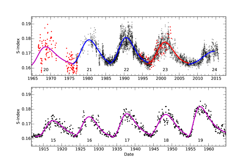
Figure 4.— Top: composite time series of nightly MWO Moon measurements (red) with daily NSO/SP data (black) converted to the MWO HKP-2 scale. Bottom: Monthly averaged $K_{\rm KKL}$ data transformed to the MWO HKP-2 scale. Cycle shape model curves are shown in red when fit using MWO data, blue when fit using only NSO/SP data, and magenta when fit using $K_{\rm KKL}$ data. Cycle numbers are shown below each cycle.

Table 2 Cycle Fit Parameters and Measurements

Cycle	$t_{\rm start}$	$t_{m}$	$B$	$\alpha\times 10^{5}$	$f_{\rm min}$	$A$	$S_{\rm min}$	$S_{\rm max}$	$\Delta S_{\rm cyc}$	$\langle S_{\rm cyc}\rangle$
15	1912.917	1917.617	2.145	7657	0.1615	0.01083	0.1615	0.172	0.0108	0.1671
16	1923.333	1927.465	1.992	5080	0.1610	0.01391	0.1614	0.175	0.0135	0.1678
17	1933.667	1937.731	1.991	9018	0.1610	0.01604	0.1610	0.177	0.0160	0.1690
18	1944.000	1948.359	2.253	4314	0.1611	0.01552	0.1619	0.177	0.0146	0.1696
19	1954.083	1957.705	1.965	12379	0.1610	0.02086	0.1610	0.182	0.0208	0.1716
20	1964.750	1968.639	2.334	7743	0.1614	0.01314	0.1621	0.174	0.0124	0.1684
21	1976.167	1980.447	2.275	3929	0.1615	0.01778	0.1629	0.179	0.0164	0.1717
22	1985.900	1990.548	2.003	4394	0.1629	0.01801	0.1631	0.181	0.0178	0.1713
23	1996.646	2001.122	2.154	3426	0.1627	0.01504	0.1634	0.178	0.0143	0.1701
24	2007.654	2014.577	2.942	1329	0.1621	0.00945	0.1626	0.172	0.0089	0.1670
$\langle 15-24\rangle$							0.1621	0.177	0.0145	0.1694
$\sigma_{\rm measure}$							0.0008	0.001	0.0012	0.0005
$\sigma_{\rm scatter}$							0.0008	0.003	0.003	0.002

We have now calibrated both the NSO/SP data and the MWO HKP-1 data to the HKP-2 scale. The complete composite time series covering cycles 20–24 is shown in top panel of Figure 4. The KKL composite (Bertello et al., 2016) allows us to further extend $S$ back to cycle 15, as shown in the bottom panel the figure. Note that the KKL data are monthly means, while the NSO/SP and MWO series are daily measurements. For each cycle we have determined the cycle duration using the absolute minimum points of a 1-yr median filter on the NSO/SP data (cycles 21–24) or using Hathaway et al. (1999) values (cycles 15–20). We have fit each cycle with a cycle shape model (equation (8)), with the best fit parameters shown in the left portion of Table 2. Cycle 24 is a special case. Because we only have observations for half of the cycle, the optimizer has difficulty obtaining a reasonable fit. This problem was resolved by constraining $\alpha$ to be a function of $t_{m}$ using the relationship found in Du (2011). From these curve fits, we determine the cycle minimum, maximum, max - min amplitude, and mean value. These results are summarized in the right portion of Table 2 and represent our best estimate of chromospheric variability through the MWO $S$-index over ten solar cycles.

The uncertainty in the cycle minima and maxima for cycle 23 were found to be $\approx$ 0.5% for cycle 23 (section 4.2), which are summed in quadrature along with the covariance term give the uncertainty in the amplitude of $\approx$ 10%. These uncertainties are then propagated into equation (12) which determines the uncertainties of the other cycles. The uncertainty in the cycle means is about 0.3%, as determined by the Monte Carlo experiment (see Appendix A). These relative uncertainties are applied to the cycle 15–24 mean in Table 2 to compute $\sigma_{\rm measure}$, the typical uncertainty cycle measurements on the $S$-index scale. The standard deviation of the minima, maxima, amplitudes and means are given as $\sigma_{\rm scatter}$.

4.7. Conversion to $\log(R^{\prime}_{\rm HK})$

The $S$-index reference bands $R$ and $V$ (equation (1)) vary with stellar surface temperature (and metalicity; see (Soon et al., 1993b)), and furthermore temperature-dependent flux from the photosphere is present in the $H$ and $K$ bands. These effects lead to a temperature dependence or “color term” in $S$ which limits its usefulness when comparing stars of varied spectral types. The activity index $R^{\prime}_{\rm HK}$ (Noyes et al. (1984)) seeks to remove the aforementioned color dependence of $S$ and is widely used in the literature. We therefore compute $\log(R^{\prime}_{\rm HK})$ of the Sun for the purpose of inter-comparison with stellar magnetic activity variations of other Sun-like stars from the MWO HK project or elsewhere. In Table 3 we used the procedure of Noyes et al. (1984) to calculate $\log(R^{\prime}_{\rm HK})$ from the $S$ measurements of Table 2. In this calculation, we adopted the solar color index $(B-V)_{\sun}=0.653\pm 0.003$ (Ramírez et al., 2012). The typical uncertainty of the cycle measurements on the $\log(R^{\prime}_{\rm HK})$ scale, $\sigma_{\rm measure}$, and standard deviation for the ten cycles, $\sigma_{\rm scatter}$, are also presented in Table 3. The cycle amplitude expressed as $\log(\Delta R^{\prime}_{\rm HK})$, and the fractional amplitude $\Delta R^{\prime}_{\rm HK}/\langle R^{\prime}_{\rm HK}\rangle$ have been used in stellar amplitude studies in the literature (Soon et al., 1994; Baliunas et al., 1996; Saar & Brandenburg, 2002).

Table 3 Cycle Measurements in $\log(R^{\prime}_{\rm HK})$

Cycle	$\log(R^{\prime}_{\rm HK,min})$	$\log(R^{\prime}_{\rm HK,max})$	$\log(\Delta R^{\prime}_{\rm HK})$	$\log(\langle R^{\prime}_{\rm HK}\rangle)$	$\Delta R^{\prime}_{\rm HK}/\langle R^{\prime}_{\rm HK}\rangle$
15	-4.9882	-4.927	-5.807	-4.9552	0.141
16	-4.9885	-4.913	-5.712	-4.9513	0.174
17	-4.9909	-4.903	-5.638	-4.9443	0.203
18	-4.9856	-4.905	-5.676	-4.9413	0.184
19	-4.9909	-4.879	-5.523	-4.9305	0.256
20	-4.9846	-4.916	-5.748	-4.9481	0.158
21	-4.9797	-4.891	-5.626	-4.9300	0.201
22	-4.9783	-4.884	-5.592	-4.9319	0.219
23	-4.9763	-4.899	-5.686	-4.9385	0.179
24	-4.9811	-4.931	-5.892	-4.9558	0.116
$\langle 15-24\rangle$	-4.9844	-4.905	-5.690	-4.9427	0.183
$\sigma_{\rm measure}$	0.0087	0.008	0.068	0.0072	0.032
$\sigma_{\rm scatter}$	0.0049	0.016	0.101	0.0093	0.038

5. Linearity of $S$ with $K$

In the above analysis we assumed that the ratio of 1 Å emission in the cores of the H & K lines, $H$ and $K$ are linearly related such that $S$ (equation (1)) and $K$ are also linear as in equation (12). It is also assumed that the pseudo-continuum bands $V$ and $R$ are constant. These assumptions were also implicit in the derivation of $S(K)$ relationships in the literature shown in Table 1, but we are not aware of any observational evidence in support of them.

We use emission indices from the SOLIS/ISS instrument ($K$, $H$) and SSS ($K$, $H$, $V$, $R$) to examine the trends with respect to the $K$ band. SOLIS/ISS emission indices are derived from spectra normalized to a single reference line profile obtained with the NSO Fourier Transform Spectrometer as described in Pevtsov et al. (2014). SSS indices are derived from continuum normalized and wavelength calibrated spectra with intensity points at 3909.3770 Å set to 0.83 and 4003.2688 Å at 0.96, and the rest of the spectrum normalized according to the line defined by those points.

Figure 5 (top) shows the relationship between the 1-Å emission index in the H and K line cores from the NSO SOLIS/ISS and Lowell SSS instruments. SOLIS/ISS data (black points) are from the beginning of observations until the middle of 2015, when the instrument moved from Kitt Peak to Tuscon and resulted in a discontinuous shift in the $K/H$ time series which is still under investigation. SSS data (green points) includes only the observations after the camera was upgraded in 2008, which is significantly less noisy than with the previous CCD. Differences in resolution and systematics such as stray light are likely responsible for the offsets in both $K$ and $H$ between the two instruments. However, in both instruments the $H(K)$ relationship is linear with a slope $b<1$ and a zero point $a>0$. The slopes found from each instrument, $\approx$ 0.8, agree to within the uncertainties. Linearity of $H$ with $K$ is compatible with the assumption of linearity of $S$ with $K$. The $H(K)$ linearity further implies that the emission ratio $K/H$ has the form:

$$\frac{K}{H}=\frac{K}{a+bK}$$ (15)

With nonzero $a$ the ratio must vary over the solar cycle. This ratio is a diagnostic of the optical depth of the surface integrated chromosphere (Linsky & Avrett, 1970). The data show that the ratio increases by $\sim 2$% over the rising phase of solar cycle 24.

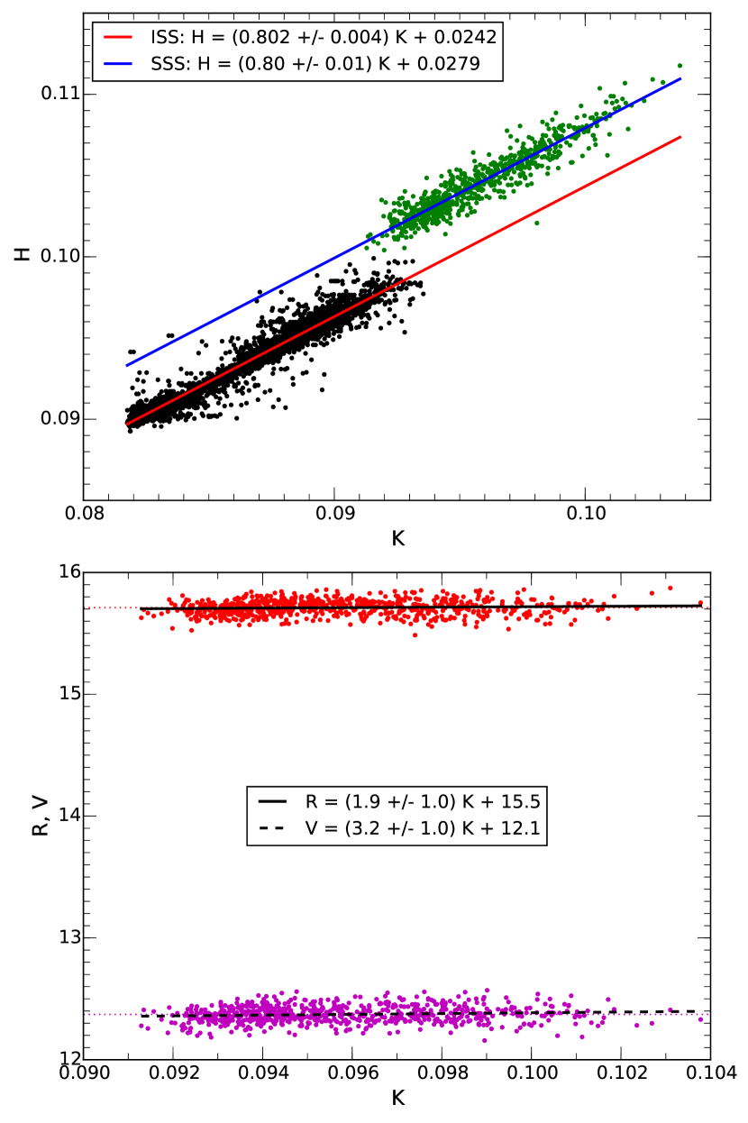
Figure 5.— Top: Relationship between calcium H & K 1-Å emission indices in SOLIS/ISS (black) and SSS (green). Bottom: $V$ and $R$ band emission indices versus $K$ from SSS spectra.

Figure 5 (bottom) shows $V$ (3891.0–3911.0 Å) and $R$ (3991.0–4011.0) Å integrated emission indices versus $K$ from continuum normalized SSS solar spectra. The data show these 20 Å pseudo-continuum bands to be nearly constant with activity, with the $V$ and $R$ bands having RMS variability of 0.6% and 0.4%, respectively. This is in agreement with the small variance in the $C_{\rm RV}$ index based on $V$ and $R$ found by Soon et al. (1993b). Linear regression of the $V(K)$ and $R(K)$ gives uncertainties in the slope (see Figure 5) that place them $3.2\sigma$ and $1.9\sigma$ from zero, respectively, giving them marginal statistical significance. The relative increase in flux indicated by these slopes for $V(K)$ and $R(K)$ over the full range of $K$ are 0.3% and 0.1% respectively.

To conclude, the data show $H$ to be linear with $K$, and $V$ and $R$ to be nearly constant, which is compatible with the model that $S=a+bK$ as assumed in the previous sections.

6. Conclusion

We have used the observations of the Moon with the MWO HKP-2 instrument to accurately place solar cycle 23 on the $S$-index scale. By deriving a proxy with the NSO/SP $K$-index data we extend the solar record to include cycles 21–24. We found that our cross-calibration method using a cycle shape model has lower uncertainty than averaging and regression methods when the number of observations is small. The Kodaikanal Observatory plage index data calibrated to the Ca K 1-Å emission index were used to calibrate the MWO HKP-1 measurements of cycle 20 to the HKP-2 scale, as well as to extend the $S$-index record back to cycle 15. The full composite time series from the KKL, HKP-1, NSO/SP, and HKP-2 instruments forms a record of chromospheric variability of the Sun over 100 years in length which may be compared to the stellar observations of the MWO and SSS programs, as well as other instrumental surveys which have accurately calibrated their data to the HKP-2 $S$ scale.

We find a mean value of $\langle S\rangle=0.1694\pm 0.0005$ for the Sun that is 4%–9% lower than previous estimates in the literature (see Table 1) that used MWO HKP-1 data or stellar observations for their calibration. We believe the discrepancy is due to (1) a systematic $+0.007$ offset in the previous $S$ calibration of the HKP-1 solar data that is within the scatter of the $F$ and $S$ relationship of Vaughan et al. (1978), and (2) uncertainties introduced in coupling those HKP-1 measurements to the non-overlapping NSO/KP and SP $K$ time series using either proxy activity time series or stellar measurements with the Lick spectrograph. This relatively small change in $S$ on the stellar activity scale (where $S$ ranges from 0.13 to 1.4 (Baliunas et al., 1995)) is a rather large fraction of the cycle amplitude, which we estimate to be $0.0145\pm 0.0014$ in $S$, on average. Our results are consistent with previous estimations from the SSS (Hall & Lockwood, 2004; Hall et al., 2007, 2009), as well as our new reduction of that dataset (see section 4.4). Our results are also consistent with parallel work by Freitas et al. (2016), who calibrate HARPS Ca ii H & K observations to the MWO $S$-index scale using an ensemble of solar twins, and found $\langle S\rangle=0.1686$ for the Sun using observations of asteroids during cycles 23 and 24.

We do not expect our change in solar $S$ to have large consequences on previous studies that used the Sun as just another star in stellar ensembles covering a wide range of rotation periods and spectral types. However, studies which used the Sun as an absolutely known anchor point in activity relationships could be significantly affected by this shift (e.g. Mamajek & Hillenbrand, 2008, who compromises and adopts the mean of Baliunas’ and Hall’s solar $S$-index in their activity-age relationship). Detailed comparisons of the Sun to solar twins will also be sensitive to this change. For example, MWO HKP-2 observations of famous solar twin 18 Sco from 1993–2003 gives a mean $S$-index of 0.173, which we find to be $\sim$2% higher than the Sun, but using other estimates from the literature we would conclude that the activity is 2%–3% lower than the Sun. This star has a measured mean rotation period of 22.7 days (Petit et al., 2008), slightly faster than the Sun, which would lead us to expect a higher activity level if in all other respects the star really is a solar twin.

Cycle amplitude is another quantity that can be compared to stellar measurements to put the solar cycle in context. So far as Ca ii H & K emission is proportional to surface magnetic flux, this gives an estimate of how much the surface flux changes over a cycle period. This $dB/dt$ is the surface manifestation of the induction equation at the heart of the dynamo problem. Soon et al. (1994) was the first to study this for the Sun and an ensemble of stars using the fractional amplitude $\Delta R^{\prime}_{\rm HK}/\langle R^{\prime}_{\rm HK}\rangle$. They found an inverse relationship between fractional amplitude and cycle period, which is also seen in the sunspot record. The fractional solar amplitude measured here has a mean value of $0.18\pm 0.03$ and ranges from 0.116 (cycle 24) to 0.255 (cycle 19). Our fractional amplitudes for cycles 21 and 22 are close to the value of 0.22 found in Soon et al. (1994) using NSO/KP data and the White et al. (1992) $S(K)$ transformation, and our range over cycles 15–24 largely overlaps with their range of values 0.06–0.17 found by transforming the sunspot record to $S$. Egeland et al. (2015) recently measured four cycle amplitudes for the active solar analog ($(B-V)=0.632$) HD 30495, with fractional amplitudes $\Delta R^{\prime}_{\rm HK}/\langle R^{\prime}_{\rm HK}\rangle$ ranging from 0.098 to 0.226 comparable to our solar measurements despite the 2.3 times faster rotation of this star. However, when using absolute amplitudes the largest HD 30495 cycle has $\Delta S=0.047$, which is 2.3 times the largest solar amplitude of 0.0211 for cycle 19. This illustrates that the use of fractional amplitudes obscures the fact that the more active, faster rotators in general have a much larger variability than the Sun, which indicates a much more efficient dynamo. Indeed, Saar & Brandenburg (2002) studied cycle amplitudes for a stellar ensemble and found that $\Delta R^{\prime}_{\rm HK}/\langle R^{\prime}_{\rm HK}\rangle\propto\langle R^{\prime}_{\rm HK}\rangle^{-0.23}$, fractional amplitude decreases with increased activity. In an upcoming work we will use the longer timeseries available today to reexamine cycle properties such as amplitude and period for an ensemble of solar analogs.

Our value of $S$ is significantly higher than the basal flux estimate of Livingston et al. (2007) of $0.133\pm 0.006$ using the center disk H + K index values from NSO/KP, transformed to the $S$-index scale using the flux relationships of Hall & Lockwood (2004). The center disk measurements integrate flux from a small, quiet region near disk center where little or no plage occurs, and the derived $S$ estimate purported to be indicative of “especially quiescent stars, or even the Sun during prolonged episodes of relatively reduced activity, as appears to have occurred during the Maunder Minimum period”. If the latter assumption were true, we estimate it would reflect an 18% reduction in $S$ from current solar minima to Maunder Minimum, or about twice the amplitude of the solar cycle. Total solar irradiance varies by $\sim$0.1% over the solar cycle (Yeo et al., 2014), so further assuming a linear relationship between $S$ and total solar irradiance this would translate into a 0.2% reduction in flux at the top of the Earth’s atmosphere. The validity of these assumptions are uncertain. Precise photometric observations of a star transitioning to or from a flat activity phase would greatly aid in determining the relationship between grand minima in magnetic activity and irradiance.

Schröder et al. (2012) measured the $S$-index for the Sun from daytime sky observations using the Hamburg Robotic Telescope (HRT) during the extended solar minimum of cycle 23–24 (2008–2009). Their instrumental $S$-index was calibrated to the MWO scale using 29 common stellar targets and published MWO measurements. They report an average $\langle S\rangle=0.153$ over 79 measurements during the minimum period, and discuss their absolute minimum $S$-index of 0.150 on several plage-free days, comparing this “basal” value to the activity of several flat-activity stars presumed to be in a Maunder Minimum-like state. Our NSO/SP $S(K)$ proxy covers the same minimum period and has an absolute minimum measurement of 0.1596 on 9 Oct 2009, while the lowest Moon measurement from the HKP-2 instrument is 0.1593 on 28 Jan 1997. Inspection of SOHO MDI magnetograms on those dates shows no significant magnetic features on the former date, while one small active region is present in the latter. The uncertainty in the calibration scale parameter from $S_{\rm HRT}$ to $S_{\rm MWO}$ (HKP-2) is about 2% Schröder et al. (2012), making their absolute minimum $S$ $\sim 2\sigma$ below ours. Baliunas et al. (1995) found a systematic error in the value and amplitude of the solar $S$-index measured from daytime sky observations, which they attributed to Rayleigh scattering in the atmosphere, ultimately deciding to omit those observations from their analysis. While Schröder et al. (2012) applied a correction for atmospheric scattering and estimated a small 0.2–1.8% error for it, we suspect that some systematic offset due to scattering remains that explains their lower $S$-index measurements.

Our results compare favorably with the independently calibrated SSS instrument at Lowell Observatory. While the MWO, NSO/SP, and NSO/KP programs have ceased solar observations, SSS continues to take observations of Ca H & K, as does the SOLIS/ISS instrument which began H & K-line observations in Dec 2006 (Bertello et al., 2011). Combining equations (5) and (12), we obtain $S(K_{\rm ISS})=1.71\,K_{\rm ISS}+0.02$, which can be used to transform data on the SOLIS/ISS scale to $S$, including the composite $K$-index dataset from 1907–present (Bertello et al., 2016; Pevtsov, 2016).

This work illustrates once again the complexities of comparing and calibrating data on several different instrumental flux scales. Some of this confusion could be avoided if more effort were put toward calibrating instruments to physical flux (erg cm^-2 s^-1). Should this be done, discussions of discrepancies would be more about the validity of the methods used to achieve the absolute calibration rather than the details of the chain of calibrations used to place measurements on a common scale. We believe the former path is preferable, though not without its own substantial difficulties. Given the encouraging agreement between the SSS and MWO HKP-2 solar and stellar data, the $S$ to flux relationships presented in Hall et al. (2007) are a good starting point for placing the MWO data on an absolute scale. Further work in this area should carefully evaluate the $S$ to flux relationship, so that calibrated Ca ii H & K flux measurements by future instruments may immediately be comparable to the extensive and pioneering Mount Wilson Observatory observations.

Thanks to Phil Judge, Giuliana de Toma, Doug Duncan, Robert Donahue, and Alfred de Wijn for the useful discussions which contributed to this work. Thanks to Steven Keil and Tim Henry for calibrating and providing NSO data products. R.E. is supported by the Newkirk Fellowship at the NCAR High Altitude Observatory. W.S. is supported by SAO grant proposal ID 000000000003010-V101. J.C.H. thanks Len Bright, Wes Lockwood and Brian Skiff for obtaining most of the SSS solar data over the years, and Len Bright for his ongoing curation of the SSS solar and stellar data. A.A.P. acknowledges the financial support by the Academy of Finland to the ReSoLVE Centre of Excellence (project no. 272157).

Appendix A: Monte Carlo Cycle Model Fitting Experiments

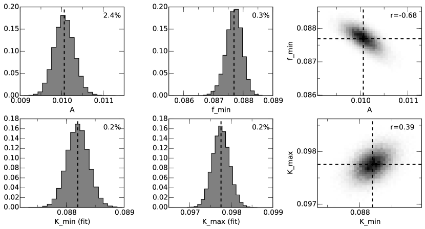
Figure 6.— Monte Carlo experiment to determine the uncertainty in cycle model amplitude and offset parameters, $\{A,f_{\rm min}\}$ (top row) and the cycle minimum and maximum $\{K_{\rm min},K_{\rm max}\}$ (bottom row) using the NSO/SP $K$-index time series for cycle 23. Distributions show results of Monte Carlo trials sampling 80% of the 1087 measurements in cycle 23. The standard deviation of each 1D distribution is shown as a percentage in the top right corner. The correlation coefficient $r=\sigma_{xy}/\sigma_{x}\sigma_{y}$ is shown in the top right corner of the 2D distributions of the right column. Each histogram is normalized by the number of trials. The “true” value from a fit using all measurements is shown with a dashed line.

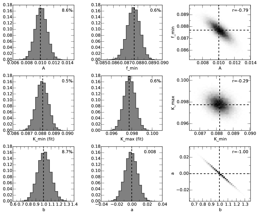
Figure 7.— Monte Carlo experiment to determine the uncertainty in the scale factor of $S(K)$ using only 56 points randomly drawn from the NSO/SP data for cycle 23. Top row: cycle shape model parameters $A$ and $f_{\rm min}$. Middle row: cycle minima and maxima determined by the model fit. Bottom row: linear transformation parameters for $K_{\rm true}=a+bK_{i}$ from the trial measurements $K_{i}$ to the true scale, $K_{\rm true}$. Each histogram is normalized by the number of trials. The “true” value from a fit using all measurements is shown with a dashed line.

In section 4.2 we used fits to the NSO/SP data and 56 MWO HKP-2 data points during the rising phase of cycle 23 to determine the minimum, maximum, amplitude and average value on the HKP-2 $S$-index scale. These fits were again used in section 4.3 to determine the $S(K)$ relationship of equation (12). We determine the uncertainty in these measurements using two Monte Carlo experiments described here.

The first experiment is aimed at understanding the uncertainties in the cycle shape fit parameters when fitting the NSO/SP $K$-index data. First, we determine the limits of cycle 23 using a 1-yr median filter on the data and taking the absolute minimum points before and after the maximum. There are 1087 NSO/SP measurements in this period. In each trial we select with replacement 80% of the measurements (N=869) and fit the cycle shape model (equation 12) parameters $\{A,t_{m},B,\alpha,f_{\rm min}\}$ to those data using the TRR+LM algorithm. In addition to the fit parameters we measure the rise phase minimum (beginning of the cycle model) and maximum value, $\{K_{\rm min},K_{\rm max}\}$.

We ran 50,000 Monte Carlo trials. The distributions for the amplitude and offset parameters, $\{A,f_{\rm min}\}$, and the cycle minima and maxima are shown in Figure 6. We computed the correlation coefficients ${\rm cov}(x,y)/(\sigma_{x}\cdot\sigma_{y})$ for all five model parameters plus the two cycle measurements, obtaining the following symmetric correlation matrix:

$$\blockarray{rrrrrrr}A&t_{m}B\alpha f_{\rm min}K_{\rm min}K_{\rm max}\\ \block{[rrrrrrr]}10.4930.303-0.158-0.684-0.6900.280\\ 10.314-0.122-0.933-0.753-0.645\\ 1-0.846-0.450-0.710-0.234\\ 10.2650.4630.163\\ 10.9140.510\\ 10.389\\ 1\\$$

The amplitude $A$ has a high negative correlation with the minima parameters, $f_{\rm min}$ and $K_{\rm min}$, indicating that high minima are compensated with low amplitudes, such that the maxima point is not too large. Indeed, there is a low correlation between $A$ and $K_{\rm max}$. In general, the minima measurement $K_{\rm min}$ is more highly correlated with the fit parameters than the maxima measurement $K_{\rm max}$ The high correlation between the time of maximum $t_{m}$ and $f_{\rm min}$ indicates that fits with early maxima have a lower minima. We are not interested in the correlations among the shape parameters ${t_{m},B,\alpha}$ as they involve time scales in the cycle which are not studied in this work.

The percent standard deviation of each quantity $x$ is $\mathbf{\sigma_{x}/\langle x\rangle}/100=(2.4,4.2,19,6.7,0.31,0.22,0.21)$, with the same ordering as in the above matrix. For $t_{m}$, we calculated $\sigma$ relative to 1 year instead of the full decimal year of maximum. We find that the standard deviation is quite small for the quantities of most concern: $\{A,f_{\rm min},K_{\rm min},K_{\rm max}\}$.

In our second Monte Carlo experiment we determine the uncertainty in fitting a partial cycle using relatively few data points, as was done for the MWO HKP-2 data for cycle 23. We take the fit to the full NSO/SP $K$-index dataset (N=1087) in cycle 23 to be the “true” cycle defined by the parameters $\{A,t_{m},B,\alpha,f_{\rm min}\}$. We then ran 50,000 Monte Carlo trials in which we randomly selected only 56 data points from the rise phase of the cycle, up to the time of the last MWO HKP-2 measurement. The selections are drawn from bins according to an N=10 equal-density binning of the MWO data points in order to ensure each trial maintained a sampling relatively uniform in time. In each trial, we randomly draw a set of cycle shape parameters $\{t_{m},B,\alpha\}$ from the previous Monte Carlo experiment. This is done in order to incorporate the uncertainty of the shape parameters into our results.

We use the same TRR+LM fitting procedure to find the remaining parameters $\{A,f_{\rm min}\}$. We compute the cycle minimum and maximum $\{K_{\rm min},K_{\rm max}\}$ from each model fit. As a check on our uncertainty derivation in equation (13) we also compute distributions of linear fit parameters $\{a_{i},b_{i}\}$ using equation (9) where the “true” values are $\{0,1\}$.

The results from the second experiment are shown in Figure 7. The percent standard deviation for the parameters $\{A,f_{\rm min},K_{\rm min},K_{\rm max}\}$ are $\{8.6,0.60,0.50,0.58\}$. We find that using only 56 data points during the rise phase increases the uncertainty in $A$ by a factor of 3.6 compared to the previous experiment. The offset parameter $f_{\rm min}$ is more robust, with the uncertainty increasing only by $\sim 65$%. The relative standard deviation for the amplitude $\Delta K=K_{\rm max}-K_{\rm min}$ was 8.4%, and that of the cycle mean $\langle K\rangle$ was 0.29%. In section 4.2, we use the relative standard deviations found in this experiment to estimate the uncertainty of $S_{\rm min}$, $S_{\rm max}$, $\Delta S$, and $\langle S\rangle$ from the 56 HKP-2 measurements of cycle 23.

Appendix B: Observations

Table 4Calibrated Solar $S$-index Time Series

Date	Original	Calibrated	Instrument
(JD $-$ 2,400,000)	$S$ or $K$	$S$
39370.857	0.177315	0.173915	MWO/HKP-1
43103.208	0.088529	0.163954	NSO/SP
49438.828	0.169500	0.169500	MWO/HKP-2
49454.496	0.164500	0.159725	SSS/CCD-1
54679.073	0.163200	0.163200	SSS/CCD-2
⋮	⋮	⋮	⋮

Note. — Table 4 is presented in its entirety in the electronic edition of the Astrophysical Journal. A portion is shown here for guidance regarding its form and content.

We provide the daily observations of solar Ca ii K or HK emissions used in this work. An example of the data are shown in Table 4. Data from five instruments are provided, denoted MWO/HKP-1, MWO/HKP-2, NSO/SP, SSS/CCD-1, SSS/CCD-2. We provide both the original calibration of the data, as an $S$-index or as the $K$-index in the case of NSO/SP, as well as the calibration to the MWO/HKP-2 scale described in this work. These data may be used to recreate Figures 1, 3, 4 (top panel), and 2. The KKL–NSO/SP–ISS composite (Bertello et al., 2016) used in the bottom panel of Figure 4 are not included here, but they are publicly available from the Harvard Dataverse (Pevtsov, 2016). Observation times are given as a modified Julian Date, and are on the UTC time scale.

References

- IAU (2015) International Astronomical Union. 2015, Resolution B3 on recommended nominal conversion constants for selected solar and planetary properties, The XXIXth International Astronomical Union General Assembly (International Astronomical Union)
- Athay (1970) Athay, R. G. 1970, ApJ, 161, 713
- Baliunas et al. (1996) Baliunas, S., Sokoloff, D., & Soon, W. 1996, ApJ, 457, L99
- Baliunas et al. (1995) Baliunas, S. L., Donahue, R. A., Soon, W. H., et al. 1995, ApJ, 438, 269
- Bertello et al. (2016) Bertello, L., Pevtsov, A., Tlatov, A., & Singh, J. 2016, Sol. Phys., arXiv:1606.01092
- Bertello et al. (2011) Bertello, L., Pevtsov, A. A., Harvey, J. W., & Toussaint, R. M. 2011, Sol. Phys., 272, 229
- Böhm-Vitense (2007) Böhm-Vitense, E. 2007, ApJ, 657, 486
- Branch et al. (1999) Branch, M. A., Coleman, T. F., & Li, Y. 1999, SIAM Journal on Scientific Computing, 21, 1
- Cayrel de Strobel (1996) Cayrel de Strobel, G. 1996, A&A Rev., 7, 243
- Donahue & Keil (1995) Donahue, R. A., & Keil, S. L. 1995, Sol. Phys., 159, 53
- Du (2011) Du, Z. 2011, Sol. Phys., 273, 231
- Duncan et al. (1991) Duncan, D. K., Vaughan, A. H., Wilson, O. C., et al. 1991, ApJS, 76, 383
- Egeland et al. (2015) Egeland, R., Metcalfe, T. S., Hall, J. C., & Henry, G. W. 2015, ApJ, 812, 12
- Freitas et al. (2016) Freitas, F. C., Meléndez, J., Bedell, M., et al. 2016, A&A, pending review
- Hall (1996) Hall, J. C. 1996, PASP, 108, 313
- Hall (2008) —. 2008, Living Reviews in Solar Physics, 5, 2
- Hall et al. (2009) Hall, J. C., Henry, G. W., Lockwood, G. W., Skiff, B. A., & Saar, S. H. 2009, AJ, 138, 312
- Hall & Lockwood (1995) Hall, J. C., & Lockwood, G. W. 1995, ApJ, 438, 404
- Hall & Lockwood (2004) —. 2004, ApJ, 614, 942
- Hall et al. (2007) Hall, J. C., Lockwood, G. W., & Skiff, B. A. 2007, AJ, 133, 862
- Harvey & White (1999) Harvey, K. L., & White, O. R. 1999, ApJ, 515, 812
- Hathaway (2015) Hathaway, D. H. 2015, Living Reviews in Solar Physics, 12, arXiv:1502.07020
- Hathaway et al. (1994) Hathaway, D. H., Wilson, R. M., & Reichmann, E. J. 1994, Sol. Phys., 151, 177
- Hathaway et al. (1999) —. 1999, J. Geophys. Res., 104, 22
- Keil et al. (1998) Keil, S. L., Henry, T. W., & Fleck, B. 1998, in Astronomical Society of the Pacific Conference Series, Vol. 140, Synoptic Solar Physics, ed. K. S. Balasubramaniam, J. Harvey, & D. Rabin, 301
- Keil & Worden (1984) Keil, S. L., & Worden, S. P. 1984, ApJ, 276, 766
- Kopp & Lean (2011) Kopp, G., & Lean, J. L. 2011, Geophys. Res. Lett., 38, L01706
- Kurucz et al. (1984) Kurucz, R. L., Furenlid, I., Brault, J., & Testerman, L. 1984, Solar flux atlas from 296 to 1300 nm
- Linsky & Avrett (1970) Linsky, J. L., & Avrett, E. H. 1970, PASP, 82, 169
- Livingston et al. (2007) Livingston, W., Wallace, L., White, O. R., & Giampapa, M. S. 2007, ApJ, 657, 1137
- Lockwood et al. (2007) Lockwood, G. W., Skiff, B. A., Henry, G. W., et al. 2007, ApJS, 171, 260
- Lockwood et al. (1997) Lockwood, G. W., Skiff, B. A., & Radick, R. R. 1997, ApJ, 485, 789
- Mamajek & Hillenbrand (2008) Mamajek, E. E., & Hillenbrand, L. A. 2008, ApJ, 687, 1264
- Meléndez et al. (2010) Meléndez, J., Schuster, W. J., Silva, J. S., et al. 2010, A&A, 522, A98
- Metcalfe et al. (2016) Metcalfe, T. S., Egeland, R., & van Saders, J. 2016, ApJ, 826, L2
- Moré (1978) Moré, J. J. 1978, in Numerical analysis (Springer), 105–116
- Noyes et al. (1984) Noyes, R. W., Hartmann, L. W., Baliunas, S. L., Duncan, D. K., & Vaughan, A. H. 1984, ApJ, 279, 763
- Petit et al. (2008) Petit, P., Dintrans, B., Solanki, S. K., et al. 2008, MNRAS, 388, 80
- Pevtsov (2016) Pevtsov, A. 2016, Composite disk-integrated Ca II K emission (EM) index of the Sun (1907-2016) (Harvard Dataverse), doi:10.7910/DVN/VF5BMO
- Pevtsov et al. (2014) Pevtsov, A. A., Bertello, L., & Marble, A. R. 2014, Astronomische Nachrichten, 335, 21
- Pevtsov et al. (2016) Pevtsov, A. A., Virtanen, I., Mursula, K., Tlatov, A., & Bertello, L. 2016, A&A, 585, A40
- Radick et al. (1998) Radick, R. R., Lockwood, G. W., Skiff, B. A., & Baliunas, S. L. 1998, ApJS, 118, 239
- Ramírez et al. (2012) Ramírez, I., Michel, R., Sefako, R., et al. 2012, ApJ, 752, 5
- Rutten (1984) Rutten, R. G. M. 1984, A&A, 130, 353
- Saar & Brandenburg (1999) Saar, S. H., & Brandenburg, A. 1999, ApJ, 524, 295
- Saar & Brandenburg (2002) —. 2002, Astronomische Nachrichten, 323, 357
- Schröder et al. (2012) Schröder, K.-P., Mittag, M., Pérez Martínez, M. I., Cuntz, M., & Schmitt, J. H. M. M. 2012, A&A, 540, A130
- Skumanich et al. (1975) Skumanich, A., Smythe, C., & Frazier, E. N. 1975, ApJ, 200, 747
- Soon et al. (1993a) Soon, W. H., Baliunas, S. L., & Zhang, Q. 1993a, ApJ, 414, L33
- Soon et al. (1994) —. 1994, Sol. Phys., 154, 385
- Soon et al. (1993b) Soon, W. H., Zhang, Q., Baliunas, S. L., & Kurucz, R. L. 1993b, ApJ, 416, 787
- Vaughan et al. (1978) Vaughan, A. H., Preston, G. W., & Wilson, O. C. 1978, PASP, 90, 267
- White & Livingston (1978) White, O. R., & Livingston, W. 1978, ApJ, 226, 679
- White & Livingston (1981) White, O. R., & Livingston, W. C. 1981, ApJ, 249, 798
- White et al. (1998) White, O. R., Livingston, W. C., Keil, S. L., & Henry, T. W. 1998, in Astronomical Society of the Pacific Conference Series, Vol. 140, Synoptic Solar Physics, ed. K. S. Balasubramaniam, J. Harvey, & D. Rabin, 293
- White et al. (1992) White, O. R., Skumanich, A., Lean, J., Livingston, W. C., & Keil, S. L. 1992, PASP, 104, 1139
- Wilson (1968) Wilson, O. C. 1968, ApJ, 153, 221
- Wilson (1978) —. 1978, ApJ, 226, 379
- Yeo et al. (2014) Yeo, K. L., Krivova, N. A., & Solanki, S. K. 2014, Space Sci. Rev., 186, 137