A dynamo model of magnetic activity in solar-like stars with different rotational velocities

Abstract

We attempt to provide a quantitative theoretical explanation for the observations that Ca II H/K emission and X-ray emission from solar-like stars increase with decreasing Rossby number (i.e., with faster rotation). Assuming that these emissions are caused by magnetic cycles similar to the sunspot cycle, we construct flux transport dynamo models of $1M_{\odot}$ stars rotating with different rotation periods. We first compute the differential rotation and the meridional circulation inside these stars from a mean-field hydrodynamics model. Then these are substituted in our dynamo code to produce periodic solutions. We find that the dimensionless amplitude $f_{m}$ of the toroidal flux through the star increases with decreasing rotation period. The observational data can be matched if we assume the emissions to go as the power 3–4 of $f_{m}$. Assuming that the Babcock–Leighton mechanism saturates with increasing rotation, we can provide an explanation for the observed saturation of emission at low Rossby numbers. The main failure of our model is that it predicts an increase of magnetic cycle period with increasing rotation rate, which is the opposite of what is found observationally. Much of our calculations are based on the assumption that the magnetic buoyancy makes the magnetic flux tubes to rise radially from the bottom of the convection zone. On taking account of the fact that the Coriolis force diverts the magnetic flux tubes to rise parallel to the rotation axis in rapidly rotating stars, the results do not change qualitatively.

bbkarak@nordita.org

1. Introduction

All late-type stars have convection zones in their outer layers and are expected to have magnetic activity due to the dynamo action taking place there. Since the dynamo action crucially depends on rotation (Parker 1955), the more rapidly rotating stars are likely to have more magnetic activity. Amongst the important observational signatures of such stellar magnetic activity are the enhanced Ca II H and K emission (Noyes et al. 1984a; Saar & Brandenburg 1999) as well as the X-ray emission (Pallavicini et al. 1981; Pizzolato et al. 2003; Wright et al. 2011), there being a good correlation between these two kinds of emission (Schrijver et al. 1992). Noyes et al. (1984a) realized that the Rossby number (the ratio of the rotation period to the convective turnover time) is a particularly convenient parameter to classify the late-type stars. In spite of some scatter, Fig. 8 of Noyes et al. (1984a) shows that the Ca II H and K emission has a functional dependence on the Rossby number—first increasing rapidly with faster rotation and then increasing more slowly for stars rotating very fast. Wright et al. (2011) present a similar pattern for the X-ray emission from the late-type stars, as seen in the right panel of their Fig. 2. They conclude that there is a power-law relation between the X-ray emission and the Rossby number for slowly rotating stars (the index being about $-$2.70), whereas the X-ray emission saturates for rapidly rotating stars.

Apart from the suggestion that these observational data can be qualitatively explained by assuming that the dynamo action becomes stronger with rotation and then probably saturates at sufficiently high rotation, detailed calculations so far have not been done. During the last few years, models of the solar dynamo have become increasingly realistic (see, for example, Charbonneau 2010; Choudhuri 2011; and references therein). The aim of the present paper is to extend our knowledge of the solar dynamo to solar-like stars rotating at different rates and explore whether the patterns of Ca II H/K and X-ray emission can be explained quantitatively.

The flux transport dynamo model has emerged in recent years as the most popular theoretical model of the Sun’s magnetic activity cycle. In this model, the toroidal field is produced by the stretching of the poloidal field by differential rotation at the bottom of the convection zone, where helioseismology has discovered a concentrated layer of differential rotation known as the tachocline. The toroidal field produced at the bottom of the convection zone rises to the solar surface due to magnetic buoyancy. The decay of tilted sunspot pairs at the solar surface gives rise to the poloidal field by what is called the Babcock–Leighton mechanism (Babcock 1961; Leighton 1964) which has received strong observational support recently (Dasi-Espuig et al. 2010; Kitchatinov & Olemskoy 2011a). The meridional circulation of the Sun plays a very important role in such dynamo models. It is observed to be poleward at the solar surface and carries the poloidal field poleward with it. To avoid piling up of matter near the sun’s poles, the meridional circulation has to have an equatorward return flow through the deeper layers of the convection zone. It is necessary for theoretical models to have such an equatorward meridional circulation at the bottom of the convection zone to cause the equatorward advection of the toroidal field generated there, in order to explain the appearance of sunspots at lower latitudes with the progress of the solar cycle (Choudhuri et al. 1995).

It is expected that solar-type stars rotating at different rates will have similar flux transport dynamos operating within their convection zones. As indicated in the last paragraph, we need a detailed knowledge of the differential rotation and the meridional circulation to model such a flux transport dynamo. For the Sun, helioseismology has provided a detailed map of the differential rotation (Schou et al. 1998), which is used in solar dynamo models. Although helioseismology provides some information about the nature of the meridional circulation in upper layers of the solar convection zone, we have no direct observational data about the return flow of meridional circulation through the deeper layers of the convection zone (but see Zhao et al. 2013; Schad et al. 2013 for some helioseismic evidence of this). Since the stable stratification in the radiation zone does not permit a considerable meridional circulation, we expect the meridional circulation to remain confined within the convection zone. By requiring $\nabla.(\rho{\bf v})=0$, one is able to come up with a reasonable distribution of the meridional circulation which, when used in solar dynamo models, gives results consistent with observations. Although some observational information about the differential rotation at the surface of stars is now available (see, for example, Berdyugina 2005; Collier Cameron 2007; Strassmeier 2009), we need detailed information about differential rotation throughout the convection zone of a star in order to construct realistic dynamo models. Such information about differential rotation or meridional circulation is not available from observational data for any stars. So, in order to construct detailed stellar dynamo models, we need to calculate the differential rotation and the meridional circulation from theoretical analysis.

Before the flux transport dynamo model of the solar cycle was proposed in 1990s (Wang et al. 1991; Choudhuri et al. 1995; Durney 1995), the importance of meridional circulation in the dynamo process was not generally recognized and there were some early efforts of constructing $\alpha\Omega$ models of stellar dynamos without including the meridional circulation (Belvedere et al. 1980; Brandenburg et al. 1994). Jouve et al. (2010) made the first comprehensive attempt of constructing flux transport models of stellar dynamos by using differential rotation and meridional circulation on the basis of 3-D hydrodynamic simulations. Isik et al. (2011) assume an interface $\alpha\Omega$ dynamo to generate magnetic fields in stars and use the meridional circulation at the stellar surface to advect the magnetic flux that has emerged there.

Global meridional flow and differential rotation in convection zones of solar-type stars can be modelled by solving jointly the mean-field equations of motion and heat transport (Brandenburg et al., 1992; Kitchatinov & Rüdiger, 1995; Küker & Stix, 2001; Rempel, 2006; Hotta & Yokoyama, 2011). Kitchatinov & Olemskoy (2011b; hereafter KO11) calculate differential rotation profiles of main-sequence dwarfs having different masses and different rotation periods. This model automatically gives rise to a meridional circulation which is essential for angular momentum balance. For a solar mass star with solar rotation period, this model gives a differential rotation profile (see Fig. 1 in KO11) remarkably close to what is found in helioseismology. The model also agrees with measurements of the surface differential rotation in rapidly rotating stars by Barnes et al. (2005). The accompanying meridional circulation consists of a single cell in the convection zone with poleward flow near the surface and equatorward flow near the bottom of the convection zone. In the present work, we use this model to compute the differential rotation and the meridional circulation of solar-like stars having different rotation periods. Then we give these as inputs in a dynamo model based on the code Surya developed in Indian Institute of Science (Nandy & Choudhuri 2002; Chatterjee et al. 2004; Karak 2010; Karak & Choudhuri 2011).

In order to avoid too many complications in this initial exploratory paper, we restrict ourselves only to stars of mass $1M_{\odot}$. Since stellar rotation slows down with age (Skumanich 1972), the sequence of solar mass stars with different rotation periods can also be viewed as a sequence of stars having different ages. The differential rotation and the meridional circulation of such stars having different rotation periods are first obtained from the model of KO11. As the star is made to rotate faster, the meridional circulation is found to be confined to the edges of the convection zone (the poleward flow in a narrow layer near the surface and the equatorward flow in a narrow layer near the bottom). However, we found that even such a meridional circulation is able to sustain a flux transport dynamo and we have been able to construct models of the dynamo operating in $1M_{\odot}$ stars having different rotation periods by putting the appropriate differential rotation and the appropriate meridional circulation in the dynamo code. The next challenging question is to connect the results of the dynamo calculation with the observed emission in Ca II H/K and X-ray.

In order to limit the growth of the magnetic field generated by the dynamo, it is necessary to include the nonlinear feedback of the growing magnetic field on the dynamo. The simplest way of doing this is to include a quenching in the $\alpha$ parameter describing the generation of the poloidal field. If the quenching is of such a nature that the dynamo action gets quenched when the toroidal field is stronger than $B_{0}$, then the maximum value of the toroidal field hovers around $B_{0}$ and the total toroidal flux in the convection zone at an instant would be $fB_{0}R_{s}^{2}$, where $f$ is usually much smaller than 1. As the toroidal field changes sign, $f$ is expected to vary in a periodic fashion going through positive and negative values. Let $f_{m}$ be the amplitude of $f$, implying that the maximum toroidal flux in the convection zone is $f_{m}B_{0}R_{s}^{2}$. In our dynamo simulations of $1M_{\odot}$ stars with different rotation periods, we find that $f_{m}$ increases with decreasing rotation periods. In other words, stars rotating faster produce more magnetic flux. The emissions in Ca II H/K or X-ray, which depend on the overall magnetic activities of the stars, are expected to increase with increasing $f_{m}$. Since the emissions (especially the X-ray emission) often arise from magnetic reconnection involving the interaction of one magnetic flux system with another, one may naively expect that the emissions may go as $f_{m}^{2}$. One of the aims of the present study is to check whether the observed dependence of the emissions on the Rossby number can be explained on the basis of such assumptions.

One assumption used in most of the dynamo models developed so far is that magnetic buoyancy makes the toroidal field at the bottom of the convection zone to rise radially through the convection zone to the solar surface. However, in the case of stars rotating sufficiently fast, the Coriolis force makes flux tubes rise parallel to the rotation axis rather than radially (Choudhuri & Gilman 1987; Choudhuri 1989; D’Silva & Choudhuri 1993; Fan et al. 1993; Weber et al. 2011). This happens when the rotation period is shorter than the dynamical time scale of the flux tube rise. If the dynamical time scale of the flux tube rise is comparable to the turnover time of convection (which is the case for the Sun), then we would expect the Coriolis force to be dominant and make flux tubes rise parallel to the rotation axis when the Rossby number is less than 1. It is intriguing that the nature of dependence of the emission on Rossby number changes around such a value, as seen in Fig. 8 of Noyes et al. (1984a) and Fig. 2 of Wright et al. (2011). The usual explanation given for such saturation is that the dynamo saturates when the rotation is fast. One important question is whether a change in the nature of the dynamo due to the change in the nature of magnetic buoyancy could also be behind this. Doppler imaging shows that some fast rotating stars have polar spots (Vogt & Penrod 1983; Strassmeier et al. 1991), which are believed to be caused by the Coriolis force diverting the rising flux tubes to high latitudes (Schüssler & Solanki 1992). But, to the best of our knowledge, no previous calculation has been done to explore how the nature of the dynamo changes when the magnetic flux rises parallel to the rotation axis rather than radially. We present some such calculations and show that the dynamo becomes less efficient and generates less magnetic flux when the toroidal field is assumed to rise parallel to the rotation axis.

One important question connected with the theory of stellar dynamos is to obtain periods of magnetic cycles. Thanks to the program of the Mount Wilson Observatory for monitoring Ca H/K emission from several solar-like stars for many years, the activity cycles of many solar-like stars have been discovered (Wilson 1978; Baliunas et al. 1995). There is evidence that stars with longer rotation periods have longer activity cycle periods. This was first reported by Noyes et al. (1984b), who pointed out that this can be easily explained for a linear $\alpha\Omega$ dynamo on the basis of some scaling arguments (see also Brandenburg et al. 1998). However, in flux transport dynamos, the cycle period is determined essentially by the time scale of the meridional circulation. Ironically, flux transport stellar dynamos have difficulty in explaining the observed increase of cycle period with the increase of rotation period (or with the decrease of rotation rate). This was pointed out by Jouve et al. (2010, see the second panel of their Figure 4), who discussed various ways of getting around this difficulty. We also encounter this difficulty in our calculations. However, in the present paper, we do not discuss possible mechanisms of solving this difficulty.

The mathematical formulation of the flux transport dynamo model is described in the next Section. In §3 we present the results obtained by assuming that the flux tubes rise radially through the convection zone due to magnetic buoyancy. Then we discuss in §4 how our results get modified when we allow the Coriolis force to make the flux tubes rise parallel to the rotation axis. Our conclusions are summarized in §5.

2. Flux transport dynamo model

We assume the magnetic field to be axisymmetric and write it in the following form:

$${\bf B}=\nabla\times[A(r,\theta){\bf e}_{\phi}]+B(r,\theta){\bf e}_{\phi}$$ (1)

where ${\bf B_{p}}=\nabla\times[A(r,\theta){\bf e}_{\phi}]$ is the poloidal component of the magnetic field and $B(r,\theta)$ is the toroidal component. Then, in the flux transport dynamo model, we solve the following equations to study the evolution of the magnetic fields:

$$\frac{\partial A}{\partial t}+\frac{1}{s}({\bf v_{p}}.\nabla)(sA)=\eta\left(\nabla^{2}-\frac{1}{s^{2}}\right)A+S(r,\theta;B),$$ (2)

$$\frac{\partial B}{\partial t}+\frac{1}{r}\left[\frac{\partial}{\partial r}(rv_{r}B)+\frac{\partial}{\partial\theta}(v_{\theta}B)\right]=\eta\left(\nabla^{2}-\frac{1}{s^{2}}\right)B$$

$$+s({\bf B}_{p}.{\bf\nabla})\Omega+\frac{1}{r}\frac{d\eta}{dr}\frac{\partial{(rB)}}{\partial{r}},~{}~{}~{}~{}~{}~{}~{}~{}~{}~{}~{}~{}~{}~{}~{}~{}~{}~{}~{}~{}~{}~{}~{}~{}~{}~{}~{}~{}~{}$$ (3)

where $s=r\sin\theta$.

Here ${\bf v_{p}}=v_{r}{\bf\hat{r}}+v_{\theta}{\bf\hat{\theta}}$ is the meridional circulation velocity, whereas $\Omega$ is the angular velocity, both ${\bf v_{p}}$ and $\Omega$ being functions of $r$ and $\theta$. The coefficient $\eta$ is the turbulent magnetic diffusivity. The Babcock–Leighton mechanism for generating the poloidal field is encaptured through the source term $S(r,\theta;B)$ in Equation (2). We shall discuss below how we specify $\eta$, $S(r,\theta;B)$, $\Omega$ and ${\bf v_{p}}$. Once these parameters are given, we have to solve Equations (2) and (3) within a hemisphere of the convection zone of the star. Since the bottom of the convection zone for solar-like stars is at $0.7R_{s}$, we carry on the numerical integration of Equations (2) and (3) within the range $0.55R_{s}<r<R_{s}$ and $0<\theta<\pi/2$, the bottom of the integration region being a little bit below the bottom of the convection zone. We now come to the boundary conditions which we use. The boundary conditions at the pole are $A=0,B=0$, and at the equator are $\partial A/\partial r=0,B=0$ which force a dipolar symmetry, whereas at the lower boundary we take $A=0,B=0$. Above the upper boundary, we assume the magnetic field to be a potential field. The upper boundary condition we use is $B=0$ and $A$ smoothly matches this potential field across the boundary (see Dikpati & Choudhuri 1995 and Chatterjee et al. 2004 for details). We use the code Surya developed at the Indian Institute of Science to solve Equations (2) and (3) with these boundary conditions (Nandy & Choudhuri 2002; Chatterjee et al. 2004; Karak 2010; Karak & Choudhuri 2011). We have used spatial resolution of $256\times 256$ for all the calculations. The code has been run for a sufficiently long time compared to the diffusion time so that the results are disregarded for the initial conditions.

We now come to the specification of the various parameters. We use the angular velocity profile $\Omega(r,\theta)$ and the meridional circulation ${\bf v_{p}}$ computed from the mean-field hydrodynamics model of KO11. The numerical model solves the steady motion equation

$$\left({\mbox{\boldmath$V$}}\cdot{\mbox{\boldmath$\nabla$}}\right){\mbox{\boldmath$V$}}+\frac{1}{\rho}\mbox{\boldmath$\nabla$}P-\mbox{\boldmath$g$}=\frac{1}{\rho}\mbox{\boldmath$\nabla$}\cdot\mbox{\boldmath$R$},$$ (4)

where the mean velocity $V$ combines the axisymmetric rotational and meridional flows, $\mbox{\boldmath$V$}=\mbox{\boldmath$e$}_{\phi}r\sin\theta\Omega+{\bf v_{p}}$ and $g$ is gravity. Convective velocities $u$ contribute the motion equation (4) via the Reynolds stress

$$R_{ij}=-\rho Q_{ij},\ \ Q_{ij}=\langle u_{i}u_{j}\rangle,$$ (5)

where $Q_{ij}$ is the correlation tensor of fluctuating velocities. Differential rotation results in the model from the angular momentum transport by convection and meridional flow. Convective fluxes of angular momentum are proportional to the correlation, $Q_{\phi r}$ and $Q_{\phi\theta}$, of azimuthal and meridional velocities. Apart from the contribution of the eddy viscosities, $Q^{\nu}_{ij}$, the correlation $Q_{ij}=Q^{\nu}_{ij}+Q^{\Lambda}_{ij}$ contains a non-viscous part, $Q^{\Lambda}_{ij}$, the presence of which in rotating fluids is named the $\Lambda$-effect (Rüdiger, 1989). It is specified after the quasi-linear theory of turbulent transport (cf. Rüdiger et al. 2013),

$$Q^{\Lambda}_{r\phi} = \frac{\tau\ell^{4}g}{15H_{\rho}c_{\mathrm{p}}}\frac{\partial S}{\partial r}\ \Omega\sin\theta\left(V(\Omega^{*})+H(\Omega^{*})\cos^{2}\theta\right),$$

$$Q^{\Lambda}_{\theta\phi} = -\frac{\tau\ell^{4}g}{15H_{\rho}c_{\mathrm{p}}}\frac{\partial S}{\partial r}\ \Omega\sin^{2}\theta\cos\theta H(\Omega^{*}),$$ (6)

where $\tau$ is the correlation time of convective turbulence, $\ell$ is the correlation length, $H_{\rho}$ is the density scale height, $c_{\mathrm{p}}$ is the specific heat capacity at constant pressure, $S$ is the specific entropy, and $V$ and $H$ are dimensionless functions of the Coriolis number $\Omega^{*}=2\tau\Omega$ (Figure 1).

Figure 1.— Normalized fluxes $V$ and $H$ of angular momentum of the Equation (6) as functions of the Coriolis number.

The entropy gradient appears in the Equation (6) because the background turbulence intensity is expressed in terms of the entropy gradient. The viscous part of the correlation reads,

$$Q^{\nu}_{ij}=-{\cal N}_{ijkl}\frac{\partial V_{k}}{\partial r_{l}}.$$ (7)

The eddy transport coefficients ${\cal N}$ are also expressed in terms of the entropy gradient which gradient in turn is controlled by the entropy equation which is solved together with the motion equation (4). This is done to reduce arbitrariness in specifying the model parameters. There only tunable parameter is $C_{\chi}$ of the eddy thermal diffusivity,

$$\chi_{ij}=-\frac{\tau\ell^{2}g}{12c_{\mathrm{p}}}\frac{\partial S}{\partial r}\left(\phi(\Omega^{*})\delta_{ij}+C_{\chi}\phi_{\|}(\Omega^{*})\hat{\Omega}_{i}\hat{\Omega}_{j}\right).$$ (8)

With this equation, the thermal diffusivities differ between the directions along and normal to the rotation axis, i.e., the diffusivity is anisotropic. The anisotropy is induced by rotation. In the limit of slow rotation, $\Omega^{*}\rightarrow 0$, the second term in the brackets of Equation (8) vanishes, $\phi_{\|}(0)=0$, and the diffusivity becomes isotropic. Finite anisotropy in a rotating star, however, is very important for its differential rotation structure. The anisotropy results in a differential temperature: a slight increase in mean temperature with latitude. The differential temperature is essential for deviation from the Taylor–Proudman state of cylinder-shaped rotation (Rüdiger et al., 2013).

The value of $C_{\chi}=1.5$ in Equation (8) gives close agreement with helioseismology. The $C_{\chi}$-parameter was, therefore, fixed to this value and not varied in stellar applications. In order to compute the differential rotation, the model needs the structure of a star to be specified. We use the EZ code of stellar evolution by Paxton (2004) to specify the structure of a $1M_{\odot}$ star as a function of age. Then, the gyrochronology relation by Barnes (2007) was used to identify the rotation rate for a star of given age. This provides a sequence of models for differential rotation and meridional flow in the Sun of different ages. All details about this modeling of stellar differential rotation can be found in KO11 and Kitchatinov & Olemskoy (2012a). The computations give solar-type rotation with the equator rotating faster than poles. Only with unrealistically slow rotation (with, say, $P_{\mathrm{rot}}=60$ days) and artificially reduced anisotropy of heat transport can the anti-solar rotation be found (Kitchatinov & Olemskoy 2012a). A similar conclusion has been reached by Gastine et al. (2014) and Karak et al. (2014a).

We point out that the model of KO11 does not include overshooting and provides the differential rotation only above $0.72R_{s}$. We assume the core of the star below $0.7R_{s}$ to rotate with the constant angular velocity $\Omega_{\rm core}$ corresponding to the rotation period used for the particular case. To produce a smooth fit between $0.7R_{s}$ and $0.72R_{s}$, we use the following procedure. Let $\Omega_{\rm model}(r,\theta)$ be equal to $\Omega$ given by the model of KO11 above $0.72R_{s}$, whereas below $0.72R_{s}$ we assume $\Omega_{\rm model}(r,\theta)$ to be equal to the value of $\Omega$ at ($r=0.72R_{s},\theta$) from the model. We now take the angular velocity to be given by the following expression

$$\Omega(r,\theta)=\Omega_{\rm model}(r,\theta)+\frac{1}{2}[\Omega_{\rm core}-\Omega_{\rm model}(r=0.72R_{s},\theta)]$$

$$\left[1-{\rm erf}\left(\frac{r-0.71R_{s}}{0.01R_{s}}\right)\right]~{}~{}~{}~{}~{}~{}$$ (9)

This expression of angular velocity implies a strong differential rotation between $0.7R_{s}$ and $0.72R_{s}$, which is our tachocline.

In this paper, we carry on calculations for $1M_{\odot}$ stars having rotation periods of 1, 2, 3, 4, 5, 7, 10, 15, 20, 25.38 (solar value) and 30 days. Figure 2 shows the angular velocity distributions of stars with rotation periods of 1, 5, 15 and 30 days. It is clear that the angular velocity tends to be constant over cylinders when the rotation is fast, whereas there is a tendency of it being constant over cones for rotation periods comparable to the solar rotation period and longer. For all the cases we computed, the meridional circulation always consists of a single cell with poleward flow near the surface and equatorward flow at the bottom of the convection zone. For faster rotations (i.e. for shorter rotation periods), the meridional circulation tends to be confined to the peripheries of the convection zone. In Figure 3, we show the streamlines of meridional circulation, whereas in Figure 4, we show $v_{\theta}$ as function of $r$ at the latitude $45^{\circ}$ for rotation periods of 1, 5, 15 and 30 days. We point out again that the model of KO11 does not include overshooting in the tachocline. As a result, the meridional circulation abruptly falls to zero at the bottom of the convection zone.

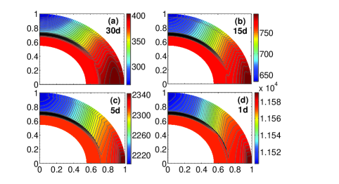
Figure 2.— The distribution of angular velocity in the poloidal planes of stars with rotation periods 30, 15, 5 and 1 days. The rotational frequencies in nHz are indicated by the different colors. Note that the lower boundary at about $0.72R_{s}$ of the KO11 model is smoothed using Equation (9) to form a tachocline-like shear layer.

Figure 3.— Streamlines of meridional circulation of stars with rotation periods 30, 15, 5 and 1 days.

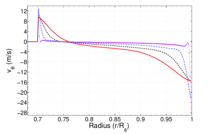
Figure 4.— The component $v_{\theta}$ (in m s^-1) of meridional circulation at $45^{0}$ latitude of four different stars. Solid (red), dashed (black), dash-dotted (blue) and dot-pointed (magenta) lines correspond to stars with rotation periods 30, 15, 5 and 1 days respectively.

The only remaining parameters to be specified are the turbulent magnetic diffusivity $\eta$ and the source term $S(r,\theta;B)$. We specify them in such a way that the code Surya gives stable periodic solutions for solar-like stars over the wide range of rotational velocities we are considering. Thus we have specified them in a way somewhat different from what we have done in some of our earlier calculations (Nandy & Choudhuri 2002; Chatterjee et al. 2004; Karak & Choudhuri 2011, 2012, 2013). With our earlier specifications of $\eta$ and $S(r,\theta;B)$, we had been able to reproduce various aspects of the solar cycle extremely well. However, we now find that these earlier specifications do not give stable periodic solutions when we use the angular velocity profile and the meridional circulation appropriate for very short rotation periods. So we use somewhat different specifications of turbulent diffusivity and magnetic buoyancy, which are very similar to what is done in other flux transport dynamo models (e.g., Muñoz-Jaramillo et al. 2009; Hotta & Yokoyama 2010). When we use these specifications for the case of solar rotation period, we find the activity cycle period to be around 6.5 yr instead of 11 yr (see Choudhuri et al. 2005 for a discussion) and the butterfly diagram also does not look very solar-like. However, here we are interested more in finding out how the behavior of the dynamo changes with different rotational velocities, rather than matching the observational data for only one value of rotational velocity (the solar value) for which we have detailed observational data. So we have used a model in which we can hold the other things invariant while changing the angular velocity profile and the meridional circulation for different rotation periods. We hope that the results obtained with this model at least qualitatively captures the changing behavior of the dynamo with different rotation periods.

We take the turbulent magnetic diffusivity to be a function of $r$ alone, having the following form:

$$\eta(r)=\eta_{\mathrm{RZ}}+\frac{\eta_{\mathrm{SCZ}}}{2}\left[1+\mathrm{erf}\left(2\frac{r-r_{\mathrm{BCZ}}}{d_{t}}\right)\right]$$

$$+\frac{\eta_{\mathrm{surf}}}{2}\left[1+\mathrm{erf}\left(\frac{r-r_{\mathrm{surf}}}{d_{2}}\right)\right]$$ (10)

with $r_{\mathrm{BCZ}}=0.7R_{s}$, $d_{t}=0.03R_{s}$, $d_{2}=0.05R_{s}$, $r_{\mathrm{surf}}=0.95R_{s}$, $\eta_{\mathrm{RZ}}=5\times 10^{8}$ cm² s^-1, $\eta_{\mathrm{SCZ}}=5\times 10^{10}$ cm² s^-1, and $\eta_{\mathrm{surf}}=2\times 10^{12}$ cm² s^-1. The radial dependence of the turbulent diffusivity is shown in Figure 5. Note that the diffusivity is weaker in the lower half of the convection zone compared to its value in the upper layers and it falls to a very low value below the convection zone. Unlike the thermal diffusivity and viscosity used in the hydrodynamics model of KO11, our turbulent magnetic diffusivity is not derived from any theory but prescribed similar to the diffusivity profile used by Muñoz-Jaramillo et al. (2009) and Hotta & Yokoyama (2010). In our all the calculations we use the same diffusivity.

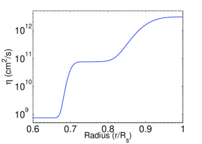
Figure 5.— Variation of turbulent diffusivity $\eta$ with stellar radius used in our dynamo model.

The source term $S(r,\theta;B)$ captures the Babcock–Leighton mechanism of the generation of the poloidal field near the stellar surface from the decay of tilted bipolar starspots. We use the following form for this term:

$$S(r,\theta;B)=\frac{\alpha(r,\theta)}{1+(\overline{B}(r_{t},\theta)/B_{0})^{2}}\overline{B}(r_{t},\theta),$$ (11)

where $\overline{B}(r_{t},\theta)$ is the value of the toroidal field at latitude $\theta$ radially averaged over the tachocline from $r=0.685R_{s}$ to $r=0.715R_{s}$. We take

$$\alpha(r,\theta)=\frac{\alpha_{0}}{4}\left[1+\mathrm{erf}\left(\frac{r-r_{4}}{d_{4}}\right)\right]\left[1-\mathrm{erf}\left(\frac{r-r_{5}}{d_{5}}\right)\right]$$

$$\times\sin\theta\cos\theta~{}~{}~{}~{}~{}~{}~{}~{}~{}~{}~{}~{}$$ (12)

with $r_{4}=0.95R_{s}$, $r_{5}=R_{s}$, $d_{4}=0.05R_{s}$, $d_{5}=0.01R_{s}$. These parameters ensure that $\alpha(r,\theta)$ is non-zero only in a thin layer near the surface, making the Babcock–Leighton mechanism operative only near the stellar surface. Following many previous authors, we carry on a non-local treatment of magnetic buoyancy by making the Babcock–Leighton mechanism operate on the magnetic field $\overline{B}(r_{t},\theta)$ in the tachocline. We have also included $\alpha$-quenching. While the $\alpha$-quenching is easier to interpret for the traditional $\alpha$-effect based on helical turbulence (Parker 1955; Steenbeck et al. 1966), we expect such quenching to be present even in the Babcock–Leighton mechanism, since a stronger magnetic field reduces the relative importance of the Coriolis force compared to the magnetic buoyancy, thereby reducing the tilt of the emerging starspot pair (D’Silva & Choudhuri 1993; Weber et al. 2011). The factor $B_{0}$ appearing in the quenching is the only nonlinearity in our model. Since the dynamo action is suppressed when the toroidal field exceeds this value, we expect the maximum value of the toroidal field in the tachocline not to exceed $B_{0}$ substantially. Essentially this $B_{0}$ should vary with different stars. However to make the calculation simple and to interpret the results clearly, we take a fixed value of $B_{0}$ for all the cases. The factor $\alpha_{0}$ in (12) determines the strength of the Babcock–Leighton process. For shorter rotation periods, the Coriolis force is stronger, making the Babcock–Leighton process also stronger by making the tilts of bipolar starspots larger. Taking the Babcock–Leighton process to be inversely proportional to the rotation period $T$, we write

$$\alpha_{0}=\alpha_{0,s}\frac{T_{s}}{T},$$

where $T_{s}$ is the solar rotation period and $\alpha_{0,s}$ is the value of $\alpha_{0}$ for the solar case, which we take $\alpha_{0,s}=1.6$ cm s^-1. We shall see in §3 that the magnetic activity keeps on rising for shorter rotation periods when we use Equation (13), instead of being saturated as seen in observational data. One possible reason behind the saturation seen in the observational data for short rotation periods is that the dynamo action gets saturated for very fast rotations. This can be phenomenologically included by replacing Equation (13) by

$$\alpha_{0}=\frac{\alpha_{0,s}}{\beta}\left[1-\exp\left(-\frac{\beta T_{s}}{T}\right)\right].$$

When we use such an expression, the Babcock–Leighton mechanism saturates when $T\ll\beta T_{s}$ and we get back Equation (13) when $T\gg\beta T_{s}$.

Finally, it should be noted that magnetic buoyancy is included in Equation (11) on the assumption that flux tubes rise radially. As we pointed out, the strong Coriolis force may make flux tubes rise parallel to the rotation axis when the rotation period is sufficiently short. We shall consider this possibility in §4, where we shall have to modify (11).

3. Results for radial rise of magnetic flux

We now present the results obtained by using the source term of the form (11), which implies that magnetic flux rises radially due to magnetic buoyancy. We first perform some simulations with a fixed Babcock–Leighton $\alpha$ and other parameters in the model. We find that the dynamo becomes weaker with the increase of rotation. The reason behind it is that the meridional circulation becomes weaker with rotation rate (see Figure 4). In flux transport dynamo model the weak meridional circulation makes the dynamo weaker due to turbulent diffusion. This effect is stronger than the increase of the shear with rotation. In other words, we can say that the $\Omega$-effect from our differential rotation does not have much role in increasing the magnetic flux. Therefore, we discuss results in which the Babcock–Leighton mechanism is assumed to vary with rotation period as Equation (13) without a saturation for rapid rotations as included in (14). Toward the end of this section, we shall point out how our results get modified on including the saturation.

We first compute the differential rotation and the meridional circulation for $1M_{\odot}$ stars with rotation periods of 1, 2, 3, 4, 5, 7, 10, 15, 20, 25.38 (solar value) and 30 days. Then we run our dynamo code for all these cases. We find that our code relaxes to give periodic solutions corresponding to activity cycles in all these cases. The butterfly diagrams obtained for the rotation periods of 1, 5, 15 and 30 days are shown in Figure 6. The contours indicate the values of the toroidal field at the bottom of the convection zone, whereas the colors indicate the values of the radial field at the stellar surface. Since starspots are expected to form when the toroidal field at the bottom of the convection zone is sufficiently strong, the contours can be taken to indicate the butterfly diagrams of starspots appearing on the surface of the star. While these butterfly diagrams tend to be confined to lower latitudes when the rotation is fast, they extend to higher latitudes for slow rotators like the Sun. While this does not fit the solar observations in detail, we find that many of the broad features of solar observations are reproduced. At lower latitudes in all the cases shown in Figure 6, we find an equatorward propagation. The toroidal field produced at the bottom of the convection zone is advected by the equatorward meridional circulation there and the poloidal field produced from it by the Babcock–Leighton mechanism also shows a tendency of equatorward shift. On the other hand, we find a poleward propagation in the higher latitudes. The poloidal field produced near the surface by the Babcock–Leighton mechanism is advected by the meridional circulation in the poleward direction at higher latitudes. Since diffusion is important in our dynamo model and the poloidal field diffuses to the bottom of the convection zone where the toroidal field is produced from it (Jiang et al. 2007), we see that the toroidal field also shows a tendency towards poleward shift at higher latitudes. This overall tendency of equatorward propagation in low latitudes and poleward propagation in high latitudes is consistent with solar observational data. It may be noted that even in detailed solar dynamo calculations it is nontrivial to confine the butterfly diagram to lower latitudes. Nandy & Choudhuri (2002) pointed out that a meridional circulation penetrating below the bottom of the convection zone helps in confining sunspot eruptions to low latitudes. Such a penetrating meridional circulation is used in the majority of solar dynamo papers from our group, but that is not the case in this paper. Some recent authors (Muñoz-Jaramillo et al. 2009; Hotta & Yokoyama 2010) used an expression for the $\alpha$-coefficient which is strongly suppressed in high latitudes, which is not done here.

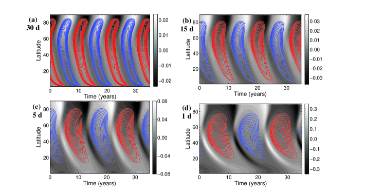
Figure 6.— Butterfly diagrams of stars with rotation periods 30, 15, 5 and 1 days. Blue (solid) contours correspond to the positive values of the toroidal field at the bottom of the convection zone, whereas red (dashed) contours correspond to the negative values of the toroidal field. The grayscale on the background shows the radial field (in the unit of $B_{0}$) on the stellar surface; white denotes the positive value and black denotes the negative.

It may be noted that the activity cycle periods for slow rotators like the Sun are somewhat shorter than the sunspot cycle periods. The reason behind this would be obvious on comparing our Figure 3 with Fig. 2 of Chatterjee et al. (2004). It is clear that the equatorward return flow of the meridional circulation in the model of KO11 is more concentrated compared to the meridional circulation we used in our solar dynamo models (Chatterjee et al. 2004; Karak 2010; Karak & Choudhuri 2011). As a result, the equatorward flow at the bottom of the convection zone in the model of KO11 which we use here is stronger than what it was in our earlier dynamo calculations. Since the cycle period in a flux transport dynamo decreases with increasing meridional circulation (Dikpati & Charbonneau 1999), it is not surprising that the meridional circulation based on the model of KO11 makes the activity cycle period somewhat shorter than what it is for the Sun. Kitchatinov & Olemskoy (2012b) found that the dynamo model based on their meridional circulation gives a cycle period closer to the sunspot period on including diamagnetic pumping, which is not included in the present calculations. In summary, the model developed in this paper, while applied to the solar case, may not fit all the observational data in quantitative detail, but the various qualitative features are broadly reproduced. The main advantage of the dynamo model presented in this paper is that it gives periodic activity cycles over a wide range of rotation periods of solar-like stars. We believe that this model gives a good idea of the general trend in the behavior of the dynamo when the rotation period is changed.

For all the rotation periods for which we have carried out dynamo calculations, we study how the total toroidal flux through the convection zone changes with time. Writing the total toroidal flux as $fB_{0}R_{s}^{2}$, we take $f$ as a measure of the total toroidal flux. Figure 7 shows the variations of $f$ with time for the rotation periods of 1, 5, 15 and 30 days. We find that the flux varies periodically going through positive and negative values, as expected from the fact that the toroidal field changes its direction from one half-cycle to the next half-cycle. It is clear from Figure 7 that the amplitude $f_{m}$ of the toroidal flux increases with decreasing rotation period (i.e. for faster rotators). To have an idea of the nature of the toroidal field generated by the dynamo, Figure 8 gives the distributions of the toroidal field at the instants when its value in the tachocline is maximum.

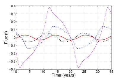
Figure 7.— Total flux $f$ of the toroidal field calculated over the whole convection zone of stars. The solid (red), dashed (black), dash-dotted (blue), and dot-pointed (magenta) lines correspond to stars with rotation periods 30, 15, 5 and 1 days respectively.

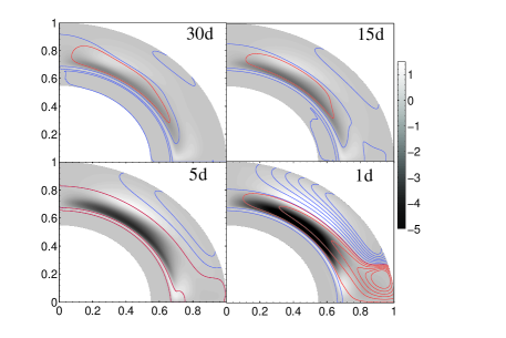
Figure 8.— Snapshot of the toroidal field (background colors) and the poloidal field (contours) when the toroidal field in the tachocline reaches the maximum value. Magnetic fields are in the unit of $B_{0}$. The four panels correspond to stars with the four different rotation periods 30, 15, 5 and 1 days. Note that same scales for the toroidal field (color) and the poloidal field (contours) are used in all the panels.

We expect more emission in Ca II H/K or in X-ray when there is more magnetic flux. Since the production of the emission usually involves magnetic reconnection of one flux system with another, we may naively expect the emission to go as the square of the magnetic flux, i.e. as $f_{m}^{2}$. Now we explore how $f_{m}^{2}$ changes with the rotation period and whether this is consistent with the observational data of Ca II H/K and X-ray emissions from solar-like stars. Noyes et al. (1984a) discovered that all the data points for Ca II H/K emission lie in a narrow range if one plots the emission against the Rossby number rather than the rotation period. In the present study, we have carried out calculations for stars with the same mass $1M_{\odot}$, for which the convective turnover time will not vary much with the rotation period. Although in the present case it would be completely satisfactory to study the variations of $f_{m}^{2}$ with the rotation period, we divide the rotation period by the convective turnover time to obtain the Rossby number $Ro$. The convective turnover time was estimated from the local mixing-length relations (cf. Eq. (8) of Kitchatinov & Olemskoy 2012a). The turnover time is depth dependent. The value for the middle of convection zone ($r=0.86R_{\mathrm{s}}$) was used to define the Rossby number. We study the variations of $f_{m}^{2}$ with the Rossby number $Ro$ so that our results can be directly compared with the observational data. The straight line (dot-dashed) in Figure 9 shows how $f_{m}^{2}$ varies with the Rossby number $Ro$. Since a straight line in this log-log plot is a good fit, we conclude that there is a power-law relation between $f_{m}^{2}$ and the Rossby number $Ro$:

$$f_{m}^{2}\propto Ro^{-\delta}.$$

Our simulations give the value $\delta\approx 1.3$, which is the slope of the straight line in Figure 9.

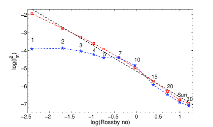
Figure 9.— Theoretically computed quantity $f_{m}^{2}$ as a function of the Rossby number, $f_{m}$ being the dimensionless amplitude of the toroidal flux over the whole convection zone. The values shown by red color (rectangle) and the linear fit (black dashed line) correspond to the case when $\alpha_{0}$ is varied according to Equation (13), whereas the values shown by blue color (star) correspond to the case when $\alpha_{0}$ is varied according to Equation (14).

The Ca II H/K data presented in Fig. 8 of Noyes et al. (1984a) or the X-ray data presented in Fig. 2 of Wright et al. (2011) can be fitted with a power law for stars with long rotation periods. We can take the luminosity as

$$L\propto Ro^{-\gamma}$$

for long rotation periods. While the canonical value of $\gamma$ is taken to be around 2, Wright et al. (2011) propose a higher value of 2.70. From Equations (15) and (16), we conclude

$$L\propto f_{m}^{2\gamma/\delta}$$

If $\gamma$ is taken to be 2, then we find $L$ to go as a power of about 3 of $f_{m}$. On the other hand, if $\gamma$ is 2.70, then $L$ would go as a higher power of $f_{m}$. It appears from our analysis that $L$ goes as a higher power of $f_{m}$ than the power 2 expected from very naive considerations. However, we are happy that, in spite of many uncertainties in our model, we get the general trend. There are ways of bringing the theoretical model closer to the observational data. We shall make some comments on this in the Conclusion. In this first exploratory study, we just present results which follow from the most obvious considerations.

As we already mentioned, the observational data show a trend of saturation for stars rotating very fast for which the Rossby number is less than 0.1 (Wright et al. 2011). In our theoretical model, we do not get any such saturation if the strength of the Babcock–Leighton mechanism is taken to be given by Equation (13). We now carry on some calculations using Equation (14) instead of Equation (13). We take $\beta T_{s}=3.6257$ days. Then we would expect a saturation for stars having rotation periods shorter than 10 days. We indeed find that, on using Equation (14) instead of Equation (13), stars with short rotation periods produce less toroidal flux. Figure 10 shows a butterfly diagram for the rotation period 5 days. This has to be compared with one of the butterfly diagrams in Figure 6. The dashed line in Figure 9 shows how $f_{m}^{2}$ varies with the Rossby number on using Equation (14) instead of Equation (13). It is clearly seen in Figure 9 that on including a saturation in the Babcock–Leighton mechanism there is a tendency of $f_{m}^{2}$ growing more slowly and reaching saturation, implying that the emission also would be saturated for fast rotators in accordance with the observational data. We thus conclude that our theoretical model is in qualitative agreement with the broad features of the observational data.

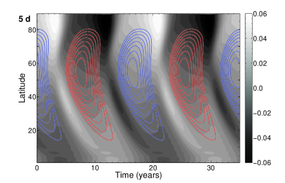
Figure 10.— Butterfly diagram of a star with rotation period of 5 days. In this case the strength of the Babcock-Leighton $\alpha$ is taken according to Equation (14).

At last, we come to the question how the activity cycle period varies with the rotation period. Figure 11 shows how the activity cycle period changes with the rotation period, the blue open circles giving the results obtained by using Equation (13) and the red solid circles giving results obtained by using (14). We find that the cycle period increases with decreasing rotation period. It is not difficult to give a physical explanation of this. Cycle period in advection-dominated dynamos is largely controlled by the meridional flow. The flow is increasingly concentrated in the boundary layers near the top and bottom of the convection zone as rotation rate increases (Figure 3). The flow velocity in the boundary layers also increases but the layers become thinner so that the flow in the bulk of the convection zone weakens. Miesch (2005) argues that angular momentum transport by meridional flow and Reynolds stress balance each other. The Reynolds stress - its viscous part as well as the $\Lambda$-effect - grow weaker than in linear proportion to the rotation rate in the rapid rotation limit due to rotational quenching of the turbulence intensity. Brown et al. (2008) found a similar trend with 3D simulations. As a result, meridional flow velocity in the bulk of convection zone decreases. Since such a meridional circulation is less effective in advecting the magnetic fields, we find longer cycles for shorter rotation periods. This theoretical result goes against the observational trend that stars with longer rotation periods tend to have longer activity cycles (Noyes et al. 1984b; Soon & Baliunas 1994). We point out that Jouve et al. (2010) also found an increase in cycle period with decreasing rotation period, exactly like what we have found, contrary to observations. However, Do Cao & Brun (2011) have found a solution of this by adding arbitrarily large latitudinal turbulent pumping in rapidly rotating stars. We believe that some important physics is still missing from our stellar dynamo models. In Conclusion we shall discuss some possibilities of closing the gap between observations and theoretical results.

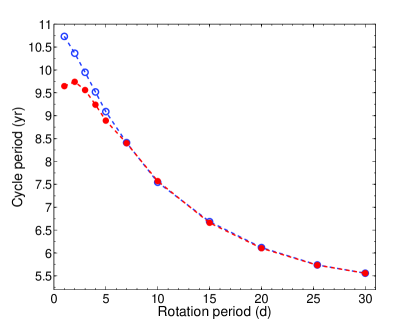
Figure 11.— Variations of the stellar activity cycle period (in years) with rotation period (in days). The blue open circles show the case when $\alpha_{0}$ is varied according to Equation (13), whereas red filled circles show the case when it is varied according to Equation (14)

4. Results for the rise of magnetic flux parallel to the rotation axis

The rise of magnetic flux tubes through the solar convection zone has been studied extensively on the basis of the thin flux tube equation (Spruit 1981; Choudhuri 1990). When the rotation period is less than the dynamical time scale of rise due to magnetic buoyancy, the Coriolis force diverts the flux tubes to rise parallel to the rotation axis (Choudhuri & Gilman 1987; Choudhuri 1989; D’Silva & Choudhuri 1993; Fan et al. 1993; Weber et al. 2011). Some mechanisms have been suggested for suppressing this effect of the Coriolis force, such as the strong interaction with the surrounding turbulence in the convection zone (Choudhuri & D’Silva 1990) or the initiation of the Kelvin–Helmholtz instability inside the flux tube (D’Silva & Choudhuri 1991). However, these mechanisms are effective only if the cross-section of the flux tube is rather small. Some of the starspots are much larger than sunspots, so these mechanisms are unlikely to be very important. Also rapidly rotating stars tend to have polar spots—presumably diverted there by the action of the Coriolis force (Schüssler & Solanki 1992).

Both the Ca II H/K emission and X-ray emission from solar-like stars tend to saturate when the Rossby number is less than about 0.1, as seen in Fig. 8 of Noyes et al. (1984a) or Fig. 2 of Wright et al. (2011). This is also approximately the Rossby number below which the rotation period is shorter than the dynamical time scale. One question which we explore here is whether the observed saturation could be caused by the effect of the Coriolis force. In all the calculations of the previous Section, we took the source function to be given by Equation (11), which implied that the flux tubes rose radially. Now, when the rotation period is less than 15 days, we replace (11) by

$$S(r,\theta;B)=\frac{\alpha(r,\theta)}{1+(\overline{B}(r_{t},\theta_{b})/B_{0})^{2}}\overline{B}(r_{t},\theta_{b}),$$

where $\overline{B}(r_{t},\theta_{b})$ is the value of the toroidal field radially averaged over the tachocline from $r=0.685R_{s}$ to $r=0.715R_{s}$ not at the latitude $\theta$ where the source function is calculated, but at the latitude $\theta_{b}$ from which a rise parallel to the rotation axis would bring to flux tube at the latitude $\theta$ when it reaches the stellar surface. We obviously have

$$r_{b}\sin\theta_{b}=R_{s}\sin\theta,$$

where $r_{b}$ is the value of $r$ at the bottom of the convection zone. When we calculate the source function for stars with rotation periods shorter than 15 days, we now use Equation (18) with $\theta_{b}$ given by (19). Since $\theta_{b}$ cannot be larger than $\pi/2$, it is clear from (19) that the source function vanishes when $\theta$ is larger than $\sin^{-1}(r_{b}/R_{s})$. In other words, the source function $S(r,\theta;B)$ is non-zero only in high latitudes and, in accordance with Equation (2), the poloidal field generation takes place only in high latitudes. Therefore by implementing this idea we expect the generation of poloidal field becomes weaker which may be responsible of producing the saturation of the Ca II H/K emission. In addition, this may make the magnetic cycle periods shorter because of restricting the dynamo in shorter domain.

In §3 we presented dynamo calculations for $1M_{\odot}$ stars with rotation periods of 1, 2, 3, 4, 5, 7, 10, 15, 20, 25.38 (solar value) and 30 days. In the cases of rotation periods of 15, 20, 25.38 (solar value) and 30 days (slow rotators), the effect of the Coriolis force is not expected to be very strong. So the magnetic flux would rise radially and the results of §3 would not change even if we take the Coriolis force into account. Only for stars with rotation periods of 1, 2, 3, 4, 5, 7 and 10 days (fast rotators), we expect the magnetic flux to rise parallel to the rotation axis when the effect of the Coriolis force is included. So we now carry on calculations only for stars with these rotation periods by using the source function given by Equations (18) and (19) rather than Equation (11).

Figure 12 presents the butterfly diagram for the rotation period of 5 days. On comparing with the butterfly diagram for this rotation period based on the assumption of radial rise, as presented in Figure 6, we find that the magnetic fields are now more confined in the higher latitudes. This is certainly expected, given that the source function now vanishes at low latitudes. However the interesting thing is that now the toroidal field is stronger at high latitudes, which can produce the polar starspots. Otherwise if the toroidal field is not stronger at high latitudes, then the magnetic flux tubes from the low latitudes go to just parallel to the rotational axis and not able to produce the polar spots.

We calculate the dimensionless toroidal flux amplitude $f_{m}$ for all the fast rotators by treating the source function according to Equations (18) and (19). Figure 13 shows a plot of $f_{m}^{2}$ as a function of the Rossby number, in which the values of $f_{m}$ for slow rotators (rotation periods of 15, 20, 25.38 and 30 days) are the same as used in Figure 9, but for fast rotators (rotation periods of 1, 2, 3, 4, 5, 7 and 10 days) $f_{m}$ is calculated by taking the source function to be given by Equations (18) and (19). For comparison we have overplotted the earlier results of the radial rise on this plot. A look at Figure 13 shows that the line joining the fast rotators gets slightly shifted below when the rise parallel to the rotation axis due to the Coriolis force is taken into account. This means that the amount of toroidal flux produced in the fast rotators is somewhat less when the magnetic flux is assumed to rise parallel to the rotation axis. This is in agreement with what we expect on the ground that the magnetic fields now occupy a smaller region (only the high latitudes) of the stellar convection zone.

Although the line for fast rotators is slightly displaced with respect to the line for slow rotators in Figure 13, we see the same trend of $f_{m}^{2}$ increasing with the Rossby number even for fast rotators that we see for slow rotators. One of our aims was to check whether the effect of the Coriolis force can explain the saturation of Ca II H/K and X-ray emission for low Rossby numbers. From Figure 11 we conclude that, although the rise parallel to the rotation axis due to the Coriolis force causes a decrease in the flux, the general trend of $f_{m}^{2}$ increasing with decreasing Rossby number is not halted by the Coriolis force. We presumably need something like the saturation of the Babcock–Leighton mechanism for fast rotation as given by Equation (10) in order to explain the observed saturation.

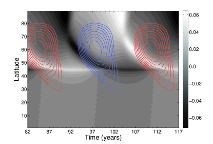
Figure 12.— Butterfly diagram of a star with rotation period of 5 days. In this case the source function is given by Equations (18) and (19) corresponding to magnetic flux rising parallel to the rotation axis.

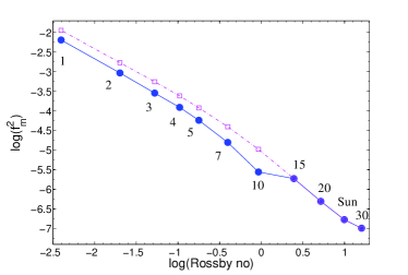
Figure 13.— The dashed line (magenta points) is the same as in Figure 9, whereas the solid line (blue points) is for the case where the source function is given by Equations (18) and (19) for rapidly rotating stars with rotation periods less than and equal to 10 days.

5. Conclusion

Following the success of the flux transport dynamo model in explaining various aspects of the solar cycle (Charbonneau 2010; Choudhuri 2011), we explore the theoretical possibility that similar flux transport dynamos operate in solar-like stars. We need profiles of the differential rotation and the meridional circulation to construct flux transport dynamo models. So we first compute these flows inside $1M_{\odot}$ stars rotating at different rates by using the mean-field hydrodynamics model of KO11. Then we use our dynamo code Surya to construct dynamo models of these stars. The only nonlinearity in our model is the standard $\alpha$ quenching which is sufficient to produce stable solutions over the parameter regime we have studied. Another possible source of nonlinearity is the back-reaction of the dynamo-generated magnetic field on the large-scale flows such as the differential rotation and the meridional circulation (see, e.g., Küker et al. 1999; Rempel 2006). In this preliminary investigation of stellar dynamos, we have not included this back-reaction. This is certainly justified for slow rotators like the Sun, on the ground that the amplitude of torsional oscillations (the cyclic variation in differential rotation) is small compared to the absolute value of the rotational velocity (Basu & Antia 2003; Howe et al. 2005; Chakraborty et al. 2009) and the variation of the meridional circulation with the solar cycle is also not so significant (Chou & Dai 2001; Hathaway & Rightmire 2010; Karak & Choudhuri 2012). However, for $1M_{\odot}$ stars rotating much faster, we have seen that the magnetic field generated is much stronger and its back-reaction may no longer be negligible. This effect should be explored in the future.

Our results are in qualitative agreement with many aspects of observational data. For example, we find that the dimensionless amplitude $f_{m}$ of the toroidal flux increases with increasing rotation. We naively expect the Ca H/K and X-ray emissions to go as $f_{m}^{2}$. We find that we can match the observational data if we assume the emissions to go as somewhat higher powers of $f_{m}$. However, if $f_{m}$ were to increase more rapidly with rotation than what is predicted by our present model, then we see from Equations (15) and (17) that it may be possible to make the emission $L$ go as $f_{m}^{2}$. We point out that we have assumed the Babcock–Leighton mechanism strength to go as $T^{-1}$ as seen in Equation (13). If we assume this strength to increase faster with increasing rotation, then we would expect to find the power law index in Equation (15) steeper. As seen from Equation (17), this would lead to a weaker dependence of $L$ on $f_{m}$. Given the many uncertainties in the theoretical model, we do not attempt such fine tuning in this paper. We merely show that the simplest possible theoretical model qualitatively gives the general trend seen in the observational data. Allowing magnetic flux to rise parallel to the rotation axis due to the Coriolis force when the rotation is faster does not change the results qualitatively.

One disagreement with observational data is that our model predicts that the magnetic cycles have longer periods when rotation periods are shorter. As we pointed out, the theoretical model of Jouve et al. (2010) also had this difficulty. We have discussed the reason behind this. The model of KO11 predicts that the meridional circulation is more confined to the peripheries of the convection zone as the star rotates faster and is less effective in advecting the magnetic fields. This less effective meridional circulation makes the period of the flux transport dynamo longer. The decrease of cycle period with faster rotation probably implies that the meridional circulation remains more effective in faster rotating stars than what our present model suggests. We have taken the anisotropy parameter $C_{\chi}$ of Equation (8) to be equal to 1.5 in all our calculations. This value of $C_{\chi}$ gives a good agreement with helioseismology for a $1M_{\odot}$ star with solar rotation. However, it is certainly possible that this anisotropy increases with faster rotation. A stronger anisotropy may make the meridional circulation more effective in faster rotating stars and thereby decrease the dynamo cycle period. We plan to explore these possibilities in future. At present, even our understanding of the meridional circulation of the Sun is fairly incomplete. There have been recent claims that the meridional circulation of the Sun may have a multi-cell structure (Zhao et al. 2013; Schad et al. 2013). Hazra et al. (2014) have shown that a flux transport dynamo can still work with a multi-cell meridional circulation as long as there is an equatorward flow at the bottom of the convection zone. All the calculations in this paper, however, are based on simple single-cell meridional circulation predicted by the model of KO11 on assuming $C_{\chi}=1.5$.

By comparing observations with the results of our preliminary theoretical studies, we find that magnetic effects probably grow somewhat faster with rotation than what is suggested by our present calculations. Only if the dimensionless amplitude $f_{m}$ of the toroidal flux increases faster with rotation, we would be able to make emission go as $f_{m}^{2}$. Probably flows inside faster rotating stars also remain stronger than what is suggested in the present model, to ensure that we have faster dynamos with shorter cycle periods. We must remember that in the present dynamo model the generation of the poloidal field from helical turbulent (the so-called $\alpha$-effect) is not included, since we know from observations that the Babcock-Leighton process is the major source of the poloidal field in the Sun. However, if this is not so true for the rapidly rotating stars and if the $\alpha$-effect starts contributing to the poloidal field generation in addition to the Babcock-Leighton process, then that can make the stellar activity stronger and can also make the cycle periods shorter. Another thing to remember is that we do not vary the turbulent diffusivity in all the calculations. However, if the turbulence is weaker in the rapidly rotating stars, possibly due to the rotational or magnetic quenching (Kitchatinov et al. 1994; Karak et al. 2014b), then the weaker turbulent diffusivity can make the dynamo stronger. Therefore, one of the aims of any future study should be to explore various effects that may make magnetic activity grow faster with rotation than what we have found. The encouraging thing is that the present calculations show the qualitative trend of magnetic activity increasing with rotation. In what ways the manifestations of stronger magnetic activity may differ from the manifestations of solar activity is another important question to be addressed. Some fast-rotating solar-like stars are known to have starspots much larger than sunspots (Strassmeier 2009). Some such stars have superflares which are much more energetic than typical solar flares (Maehara et al. 2012). One related question is whether solar flares substantially more energetic than the flares recorded so far are possible in the Sun (Shibata et al. 2013).

In this paper, we have restricted ourselves to studying only the regular aspects of stellar activity cycles. The observational data of stellar activity presented by Baliunas et al. (1995) (also see Baliunas & Soon 1995) show that many stellar cycles show strong irregularities. Constructing theoretical models of irregularities of the solar cycle has been a major research activity in the field of solar dynamo theory in recent years. Studying the irregularities of stellar cycles presumably will be a fertile research field for the future. One intriguing question is whether irregularities of stellar cycles show patterns similar to solar cycle irregularities. One important aspect of the solar cycle irregularities is the Waldmeier effect (Waldmeier 1935) that stronger cycles tend to have shorter rise times. The data of Baliunas et al. (1995) do not cover a long enough time interval to conclusively ascertain whether stellar cycles also show the Waldmeier effect. However, for a few stars, the time variation plots of Ca H emission presented by Baliunas et al. (1995) cover several cycles. If we carefully look at the Baliunas et al. (1995) plots of some stars—notably HD 103095 (in Fig. 1e), HD 149661 and HD 26965 (in Fig. 1f), HD 4628, HD 201091 and HD 32147 (in Fig. 1g)—we see tantalizing hints that stronger cycles tend to rise faster, suggesting that the Waldmeier effect is present in stellar dynamos as well. Karak & Choudhuri (2011) have shown how fluctuations in the meridional circulation can give rise to the Waldmeier effect in a flux transport dynamo. The tentative hint of the Waldmeier effect in stellar cycles certainly suggests that the meridional circulations inside solar-like stars also probably have large fluctuations. Apart from fluctuations in the meridional circulation, the other source of irregularities in the solar cycle is fluctuations in the Babcock–Leighton process (Choudhuri et al. 2007; Choudhuri & Karak 2009; Olemskoy et al. 2013). The combined fluctuations in the meridional circulation and the Babcock–Leighton mechanism can explain various aspects of grand minima in solar activity rather elegantly (Choudhuri & Karak 2012; Karak & Choudhuri 2013). The data of Baliunas et al. (1995) show grand minima phases of several stars. Presumably the physics behind these stellar grand minima is the same as the physics behind solar grand minima. We hope that detailed studies of irregularities in stellar dynamos will be carried out in the future.

References

- Babcock (1961) Babcock, H. W. 1961, ApJ, 133, 572
- Barnes et al. (2005) Barnes, J. R., Collier Cameron, A., Donati, J.-F., James, D. J., Marsden, S. C., & Petit, P. 2005, MNRAS, 357, L1
- Baliunas et al. (1995) Baliunas, S. L., et al. 1995, ApJ, 438, 269
- Baliunas & Soon (1995) Baliunas, S. Soon, W. ApJ, 1995, 450, 896
- Barnes (2007) Barnes, S. A. 2007, ApJ, 669, 1167
- Basu & Anti (2003) Basu, S., & Antia, H. M. 2003, ApJ, 585, 553
- Belvedere (1889) Belvedere, G., Paterno, L., & Stix, M. 1980, A&A, 91, 328
- Berdyugina (2005) Berdyugina, S. V. 2005, LRSP, 2, 8
- Brandenburg et al. (1992) Brandenburg, A., Moss, D., & Tuominen, I. 1992, A&A, 265, 328
- Brandenburg et al. (1994) Brandenburg, A., Charbonneau, P., Kitchatinov, L. L., & Rüdiger, G. 1994, in Cool Stars, Stellar Systems, and the Sun, ed. J.-P. Caillault, ASP Conf. Ser., 64, 354
- Brandenburg et al. (1998) Brandenburg, A., Saar, S. H. & Turpin, C. R. 1998, ApJ, 498,L51
- Brown et al. (2008) Brown, B. P., Browning, M. K., Brun, A. S., Miesch, M. S., & Toomre, J. 2008, ApJ, 689, 1354
- Chakraborty et al. (2009) Chakraborty, S., Choudhuri, A. R. & Chatterjee, P. 2009, Phys. Rev. Lett. 102, 041102
- Charbonneau (2010) Charbonneau, P. 2010, LRSP, 7, 3
- Chatterjee et al. (2004) Chatterjee, P., Nandy, D., & Choudhuri, A. R. 2004, A&A, 427, 1019
- Chou & Dai (2001) Chou, D.-Y., & Dai, D.-C. 2001, ApJ, 559, 175
- Choudhuri (1989) Choudhuri, A. R. 1989, Sol. Phys. 123, 217
- Choudhuri (1990) Choudhuri, A. R. 1990, A&A, 239, 335
- Choudhuri (2011) Choudhuri, A. R. 2011, Pramana, 77, 77
- Choudhuri et al. (2007) Choudhuri, A. R., Chatterjee, P., & Jiang, J. 2007, Phys. Rev. Lett., 98, 131103
- Choudhuri & D’Silva (1990) Choudhuri, A. R. & D’Silva, S. 1990, A&A, 239, 326
- Choudhuri & Gilman (1987) Choudhuri, A. R., & Gilman, P. A. 1987, ApJ, 316, 788
- Choudhuri & Karak (2009) Choudhuri, A. R., & Karak, B. B. 2009, RAA, 9, 953
- Choudhuri & Karak (2012) Choudhuri, A. R., & Karak, B. B. 2012, Phys. Rev. Lett., 109, 171103
- Choudhuri et al. (2005) Choudhuri, A. R., Nandy, D., & Chatterjee, P. 2005, A&A, 437, 703
- Choudhuri et al. (1995) Choudhuri, A. R., Schüssler, M., & Dikpati, M. 1995, A&A, 303, L29
- Collier Cameron (2007) Collier Cameron, A. 2007, AN, 328, 1030
- D’Silva & Choudhuri (1991) D’Silva, S., & Choudhuri, A. R. 1991, Sol. Phys., 136, 201
- D’Silva & Choudhuri (1993) D’Silva, S., & Choudhuri, A. R. 1993, A&A, 272, 621
- Dasi-Espuig et al. (2010) Dasi-Espuig, M., Solanki, S. K., Krivova, N. A., Cameron, R. & Peñuela, T. 2010, A&A, 518, 7
- Dikpati & Charbonneau (1999) Dikpati, M., & Charbonneau, P. 1999, ApJ, 518, 508
- Dikpati & Choudhuri (1995) Dikpati, M., & Choudhuri, A. R. 1995, Sol. Phys., 161, 9
- Do Cao & Brun (2011) Do Cao, O. & Brun, A. S. 2011, AN, 332, 907
- Durney (1995) Durney, B. R. 1995, Sol. Phys., 160, 213
- Fan et al. (1993) Fan, Y., Fisher, G. H., & Deluca, E. E. 1993, ApJ, 405, 390
- Gastine et al. (2014) Gastine, T., Yadav, R. K., Morin, J., Reiners, A., & Wicht, J. 2014, MNRAS, 438, L76
- Hathaway & Rightmire (2010) Hathaway, D. H., Rightmire, L. 2010, Science, 327, 1350
- Hazra et al. (2014) Hazra, G., Karak, B. B. & Choudhuri, A. R. 2014, ApJ, 782, 93
- Hotta & Yokoyama (2010) Hotta, H., & Yokoyama, T. 2010, ApJ, 714, L308
- Hotta & Yokoyama (2011) Hotta, H., & Yokoyama, T. 2011, ApJ, 740, 12
- Howeet al. (2005) Howe, R., Christensen-Dalsgaard, J., Hill, F., Komm, R., Schou, J., & Thompson, M. J. 2005, ApJ, 634, 1405
- Isik et al. (2011) Isik, E., Schmitt, D., & Schüssler, M. 2011, A&A, 528, 135
- Jiang et al. (2007) Jiang, J., Chatterjee, P., & Choudhuri, A. R. 2007, MNRAS, 381, 1527
- Jouve et al. (2010) Jouve, L., Brown, B. P., & Brun, A. S 2010, A&A, 509, 32
- Karak (2010) Karak, B. B. 2010, ApJ, 724, 1021
- Karak & Choudhuri (2011) Karak, B. B., & Choudhuri, A. R. 2011, MNRAS, 410, 1503
- Karak & Choudhuri (2012) Karak, B. B., & Choudhuri, A. R. 2012, Sol. Phys., 278, 137
- Karak & Choudhuri (2013) Karak B. B., & Choudhuri, A. R. 2013, RAA, 13, 1339
- Karak et al. (2014a) Karak, B. B., & Käpylä, P. J., Mantere, M. J., Brandenburg, A. 2014a, A&A, submitted, arXiv:1407.0984
- Karak et al. (2014b) Karak B. B., & Rheinhardt, M., Brandenburg, A., Käpylä, P. & Mantere, M. J. 2014b, ApJ, submitted, arXiv:1406.4521
- Kitchatinov et al. (1994b) Kitchatinov, L. L., Pipin, V. V. & Rüdiger, G. 1994, AN, 315, 157
- Kitchatinov & Olemskoy (2011a) Kitchatinov, L. L., & Olemskoy, S. V. 2011a, Astronomy Letters, 37, 656
- Kitchatinov & Olemskoy (2011b) Kitchatinov, L. L., & Olemskoy, S. V. 2011b, MNRAS, 411, 1059 (KO11)
- Kitchatinov & Olemskoy (2012a) Kitchatinov, L. L., & Olemskoy, S. V. 2012a, MNRAS, 423, 3344
- Kitchatinov & Olemskoy (2012b) Kitchatinov, L. L., & Olemskoy, S. V. 2012b, Sol. Phys. 276, 3
- Kitchatinov & Rüdiger (1995) Kitchatinov, L. L., & Rüdiger, G. 1995, A&A, 299, 446
- Küker & Stix (2001) Küker, M. & Stix, M. 2001, A&A, 366, 668
- Küker et al. (1999) Küker, M., Arlt, R., Rüdiger, G. 1999, A&A, 343, 977
- Leighton (1964) Leighton, R. B. 1964, ApJ, 140, 1547
- Maehara et al. (2012) Maehara, H. et al. 2012, Nature, 485, 478
- Miesch (2005) Miesch, M. S. 2005, LRSP, 2, 1
- Muñoz-Jaramillo et al. (2009) Muñoz-Jaramillo, A., Nandy, D., & Martens, P. C. H. 2009, ApJ, 698, 461
- Nandy & Choudhuri (2002) Nandy, D., & Choudhuri, A. R. 2002, Science, 296, 1671
- Noyes et al. (1984a) Noyes, R. W., Hartmann, L. W., Baliunas, S. L., Duncan, D. K., & Vaughan, A. H. 1984a, ApJ, 279, 763
- Noyes et al. (1984b) Noyes, R. W., Weiss, N. O., & Vaughan, A. H. 1984b, ApJ, 287, 769
- Olemskoy et al. (2013) Olemskoy, S. V., Choudhuri, A. R., & Kitchatinov, L. L. 2013, Astronomy Reports, 57, 458
- pallavicini (19281) Pallavicini, R., Golub, L., Rosner, R., Vaiana, G. S., Ayres, T., & Linsky, J. L. 1981, ApJ, 248, 279
- Parker (1955) Parker, E. N. 1955, ApJ, 122, 293
- Paxton (2004) Paxton, B. 2004, PASP, 116, 699
- Pizzolato (2003) Pizzolato, N., Maggio, A., Micela, G., Sciortino, S., & Ventura, P. 2003, A&A, 397, 147
- Rempel (2005) Rempel, M. 2005, ApJ, 622, 1320
- Rempel (2006) Rempel, M. 2006, ApJ, 647, 662
- Rüdiger (1989) Rüdiger, G. 1989, Differential Rotation and Stellar Convection (Berlin: Akademie-Verlag)
- Rüdiger et al. (2013) Rüdiger, G., Kitchatinov, L. L., & Hollerbach, R. 2013, Magnetic Processes in Astrophysics (Weinheim: WILEY-VCH)
- Saar & Brandenburg (1999) Saar, S. H. & Brandenburg, A., 1999, ApJ, 524, 295
- Schad et al. (2013) Schad, A., Timmer, J., & Roth, M. 2013 ApJL, 778, L38
- Schou et al. (1998) Schou, J., Antia, H. M., Basu, S., et al. 1998, ApJ, 505, 390
- schrijver (1992) Schrijver, C. J., Dobson, A. K., & Radick, R. R. 1992, A&A, 258, 432S
- Schüssler & Solanki (1992) Schüssler, M. & Solanki, S. K. 1992, A&A, 264, L13
- Shibata et al. (2013) Shibata, K. et al. 2013, PASJ, 65, 49
- Skumanich (1972) Skumanich, A., 1972 ApJ, 171, 565
- Soon & Baliunas (1994) Soon W. H. Baliunas, S. L. Sol. Phys. 1994, 154, 385
- Spruit (1981) Spruit, H. C. 1981, A&A, 98, 155
- Steenbeck et al. (1966) Steenbeck, M., Krause, F., & Rädler, K.-H. 1966, Z. Naturforsch., 21a, 1285
- Strassmeier (2009) Strassmeier, K. G. 2009, A&ARv, 17, 251
- strassmeier (1991) Strassmeier, K. G., Rice, J. B., Wehlau, W. H., Vogt, S. S., Hatzes, A. P., Tuominen, I., Hackman, T., Poutanen, M., & Piskunov, N. E. 1991, A&A, 247, 130
- vogt (1983) Vogt, S. S., & Penrod, G. D. 1983, PASP, 95, 565
- Waldmeier (1935) Waldmeier M., 1935, Mitt. Eidgen. Sternw. Zurich, 14, 105
- Wang et al. (1991) Wang, Y.-M., Sheeley, N. R., & Nash, A. G. 1991, ApJ, 383, 431
- Weber et al. (2011) Weber, M. A., Fan, Y. & Miesch, M. S. 2011, ApJ, 741, 11.
- Wilson (1987) Wilson, O. C. 1978, ApJ, 226, 379
- Wright et al. (2011) Wright, N. J., Drake, J. J., Mamajek, E. E. & Henry, G. W. 2011, ApJ, 743, 48
- Zhao et al. (2013) Zhao, J., Bogart, R. S., Kosovichev, A. G., Duvall, T. L., & Hartlep, T. 2013, ApJ, 774, L29