Dynamo cycles in global convection simulations of solar-like stars

Abstract

Context. Several solar-like stars exhibit cyclic magnetic activity similar to the Sun as found in photospheric and chromospheric emission.

Aims. We want to understand the physical mechanism involved in rotational dependence of these activity cycle periods.

Methods. We use three-dimensional magnetohydrodynamical simulations of global convective dynamos models of solar-like stars to investigate the rotational dependency of dynamos. We further apply the test-field method to determine the $\alpha$ effect in these simulations.

Results. We find dynamo with clear oscillating mean magnetic fields for moderately and rapidly rotating runs. For slower rotation, the field is constant or exhibit irregular cycles. In the moderately and rapidly rotating regime the cycle periods increase weakly with rotation. This behavior can be well explained with a Parker-Yoshimura dynamo wave traveling equatorward. Even though the $\alpha$ effect becomes stronger for increasing rotation, the shear decreases steeper, causing this weak dependence on rotation. Similar as other numerical studies, we find no indication of activity branches as suggested by Brandenburg et al. (1998). However, our simulation seems to agree more with the transitional branch suggested by Distefano et al. (2017) and Olspert et al. (2017). If the Sun exhibit a dynamo wave similar as we find in our simulations, it would operate deep inside the convection zone.

1 Introduction

The Sun, our nearest late-type star exhibits a magnetic activity cycle with a period of around 11 yrs. The cyclic magnetic field is generated by a dynamo operating below the surface, where it converts the energy of rotating convective turbulence into magnetic energy. The solar dynamo mechanism is still far from being fully understood (e.g. Ossendrijver 2003; Charbonneau 2014). One reason is the limited information about the dynamics in the solar convection zone. Helioseismology have provided us with the profile of temperature and density stratification and the differential rotation (e.g. Schou et al. 1998) in the interior, further information such as the meridional circulation profiles, convective velocity strength or even magnetic field distributions are currently inconclusive or not even possible (e.g. Basu 2016; Hanasoge et al. 2016). One way to investigate how important differential rotation, meridional circulation and turbulent convective velocities are for the solar dynamo, is to use numerical simulations. Since the early simulations by Gilman (1983), there have been several advances using numerical simulation due to the increase of computing resources. Nowadays, global simulations of convective dynamos are able to reproduce cyclic magnetic fields and dynamo solutions resembling many features of the solar magnetic field evolution (Ghizaru et al. 2010; Käpylä et al. 2012; Warnecke et al. 2014; Augustson et al. 2015), even the long-time evolution (Augustson et al. 2015; Käpylä et al. 2016; Beaudoin et al. 2016). The cyclic magnetic field in these simulations can be well understood in terms of Parker-Yoshimura rule (Parker 1955; Yoshimura 1975; Warnecke et al. 2014), where a propagating $\alpha\Omega$ dynamo wave is excited, see also Gastine et al. (2012). The $\alpha$ effect (Steenbeck et al. 1966) describes the magnetic field enhancement from helical turbulence and the $\Omega$ effect the shearing of magnetic field caused by the differential rotation. The propagation direction of the dynamo wave depends on the sign of $\alpha$ and shear: for generating an equatorward propagating wave, the product of $\alpha$ and the radial gradient of $\Omega$ must be negative (positive) in the northern (southern) hemisphere. For explaining the solar equatorward propagation of the sunspot appearance by the Parker-Yoshimura rule therefore requires either to invoke the near-surface-shear layer (Brandenburg 2005), because only there the radial gradient is negative (Barekat et al. 2014) and $\alpha$ is positive or that $\alpha$ changes sign in the bulk of the convection zone (Duarte et al. 2016), where the radial shear is positive. Furthermore, to fully understand the magnetic field evolution in the global numerical simulation one needs suitable analysis tools to extract the important contribution of turbulent dynamo effects. One of these tools is the test-field method (Schrinner et al. 2005, 2007; Warnecke et al. 2018). This method allows to determine the turbulent transport coefficients directly from the simulations. This include the measurement of tensorial coefficients such as $\alpha$, turbulent pumping and turbulent diffusion. Already the first application to global convection simulation of solar-like dynamo revealed that the turbulent effects can have a significant impact on the large-scale magnetic field dynamics (Warnecke et al. 2018; Gent et al. 2017).

Another possibility to understand the solar dynamo make use of the observation of other stars. Since the Mount Wilson survey, we know that many stars exhibit cyclic magnetic activity (e.g. Noyes et al. 1984a, b; Baliunas et al. 1995). In this survey, they observe solar-like stars in the chromospheric Ca II H&K band, which is used as a proxy for magnetic activity. Using this data Brandenburg et al. (1998) and Saar & Brandenburg (1999) found two distinguish branches, when they plot the ratio of rotational period and activity cycle period $P_{\rm rot}/P_{\rm cycl}$ over the rotational influence on the stellar convection in terms of the inverse Rossby number. The two branches are called inactive and active branch, because of their preferred magnetic activity, divided by the so-called Vaughan–Preston gap (Vaughan & Preston 1980). Their slopes are positive in terms of rotational influence, this means the cycle period decreases faster than linear with increasing rotation. This agrees qualitatively with the finding of Noyes et al. (1984b), where they obtain $P_{\rm cycl}\propto P_{\rm rot}^{1.25}$. However, Oláh et al. (2016) find in their recent re-analysis of the Mount Wilson data a relation of $P_{\rm cycl}\propto P_{\rm rot}^{0.24}$. The activity branches of Brandenburg et al. (1998) have been recently supported (Brandenburg et al. 2017), but also questioned (Reinhold et al. 2017; Distefano et al. 2017; Boro Saikia et al. 2018; Olspert et al. 2017). One of the short comings is clearly the use of the ill-determine convective turnover time $\tau_{c}$, which is used to the calculated the Rossby number $\mbox{\rm Ro}=4\pi P_{\rm rot}/\tau_{c}$; for every star $\tau_{c}$ is highly depth-dependent and different location of a dynamo might invoke a different $\tau_{c}$. However, these branches can be also obtained using the fractional Ca II H&K emission $R^{\prime}_{\rm HK}$ instead of the Rossby number (see e.g. Brandenburg et al. 2017; Olspert et al. 2017).

Explaining the observational findings via dynamo models has been challenging. Simple mean-field models of turbulent dynamos produce rotational dependencies of cycle period similar to the observed ones using overlapping induction layers (Kleeorin et al. 1983). Advective dominated flux transport models tend to produce an increase of cycle periods with increasing rotation rate (e.g. Dikpati & Charbonneau 1999; Bonanno et al. 2002; Jouve et al. 2010), which is opposite what is observed. In these models the cycle length is mainly determined by the strength of return flow of the meridional circulation, which is believed to decreases with increasing rotation (e.g. Köhler 1970; Brown et al. 2008; Warnecke et al. 2016; Käpylä et al. 2017; Viviani et al. 2018). However, the models of Kitchatinov & Rüdiger (1999) show an increase of meridional circulation strength with rotation, leading to a decrease of cycle period with rotation (e.g. Küker et al. 2001), which agrees qualitatively with observations.

Another possibility to explain cycles in dynamo models is via the turbulent (eddy) magnetic diffusivity. In a propagating $\alpha\Omega$ dynamo wave, the dynamo drivers, whose are responsible for the cycle length, have to balance with the contribution from the turbulent diffusion. Using a turbulent diffusivity of $\eta_{\rm t}=2\times 10^{8}\,\rm m^{2}/s$ one gets a magnetic cycle length of around 23 yrs (e.g. Roberts & Stix 1972), which is pretty close to solar value of 22 yrs. A change in the cycle length can be then associated with a change in the turbulent diffusion caused by magnetic or rotational quenching (e.g. Rüdiger et al. 1994). These authors found a cycle dependence of $P_{\rm cycl}\propto P_{\rm rot}^{0.1}$.

There has been only a limited number of studies of rotational dependencies of dynamo cycles using global dynamo simulation. Strugarek et al. (2017) found $P_{\rm cycl}\propto P_{\rm rot}^{-1.06}$ in a rather limited sample of rotation rates. In the recent work by Viviani et al. (2018), the author found no clear dependency of cycle periods with rotation. However, a decrease in cycle period with increasing rotation seems be more likely than an increase, which might be because of the strong oscillatory non-axisymmetric magnetic fields in these simulations.

In this work, we present the results of spherical convective dynamo models with rotation rates varying by a factor of 30. We will determine the cycle dependency on rotational influence, see Section 3.1, interpreted the data in terms of the Parker-Yoshimura rule by using test-field obtained transport coefficients, see Section 3.2, and compare the finding with observational as well as other numerical results in Section 3.3.

2 Model and setup

The detailed description of the general model can be found in Käpylä et al. (2013) and will not be repeated here. We model the convection zone of a solar-like star in spherical polar coordinates ($r,\theta,\phi$) using the wedge assumption $0.7\,R<r<R$, $\Theta_{0}<\theta<\pi-\Theta_{0}$ and $0<\phi<\pi/2$ with $R$ being the stellar radius and $\Theta_{0}=15^{\circ}$. We solve the evolution equations of compressible magnetohydrodynamics for the magnetic vector potential $A$, which therefore ensures the solenoidality of the magnetic field $\mbox{\boldmath$B$}{}=\mbox{\boldmath$\nabla$}{}\times\mbox{\boldmath$A$}{}$, for the velocity $u$, the specific entropy $s$ and density $\rho$. The model assumes an ideal gas for the equation of state. The fluid is also influenced by Keplerian gravity and rotation via the Coriolis force. Because of the wedge assumption, we use periodic boundary condition in the azimuthal ($\phi$) direction. We assume a stress-free condition for the velocity field at other boundaries and perfect conducting latitudinal and bottom boundaries and radial field condition at the top boundary for the magnetic field. The energy is transported into the system via a constant heat flux at bottom boundary and the temperature obeys a black body condition. On the latitudinal boundaries, the energy flux is vanishing using zero derivative for the thermal-dynamical quantities. The detailed setup including the exact equations and expression for the boundary condition can be found in Käpylä et al. (2013, 2017) and Warnecke et al. (2014).

We characterize our runs with the following non-dimensional input parameters; the Taylor number, the SGS, and magnetic Prandtl numbers

$$\mbox{\rm Ta}=[2\Omega_{0}(0.3R)^{2}/\nu]^{2},\quad\mbox{\rm Pr}_{\rm SGS}={\nu\over\chi_{\rm m}^{\rm SGS}},\quad\mbox{\rm Pr}_{\rm M}={\nu\over\eta},$$ (1)

where $\nu$ and $\eta$ are the constant kinematic viscosity and magnetic diffusivity, and the sub-grid-scale (SGS) heat diffusivity $\chi_{\rm m}^{\rm SGS}=\chi_{\rm SGS}(r_{\rm m})$ is evaluated at $r_{\rm m}=0.85R$. Furthermore, we use the Rayleigh number obtained from the hydrostatic stratification, evolving a 1D model, given by

$$\mbox{\rm Ra}\!=\!\frac{GM(0.3R)^{4}}{\nu\chi_{\rm m}^{\rm SGS}R^{2}}\bigg{(}-\frac{1}{c_{\rm P}}\frac{{\rm d}s_{\rm hs}}{{\rm d}r}\bigg{)}_{(r=0.85R)},$$ (2)

where $s_{\rm hs}$ is the hydrostatic entropy. As diagnostic parameters, we quote the density contrast.

$$\Gamma_{\rho}\equiv\rho(r=0.7R)/\rho(R),$$ (3)

the fluid and magnetic Reynolds numbers and the Péclet number,

$$\mbox{\rm Re}=\frac{u_{\rm rms}}{\nu k_{\rm f}},\quad\mbox{\rm Re}_{\rm M}=\frac{u_{\rm rms}}{\eta k_{\rm f}},\quad\mbox{\rm Pe}=\frac{u_{\rm rms}}{\chi_{\rm m}^{\rm SGS}k_{\rm f}},$$ (4)

where $k_{\rm f}=2\pi/0.3R\approx 21/R$ is an estimate of the wavenumber of the largest eddies. We defined the Coriolis number as

$$\mbox{\rm Co}=2\Omega_{0}\tau_{c}\equiv\mbox{\rm Ro}^{-1},$$ (5)

where $\tau_{c}=1/u_{\rm rms}k_{\rm f}$ is the convective turnover time and $u_{\rm rms}=\sqrt{(3/2)\langle u_{r}^{2}+u_{\theta}^{2}\rangle_{r\theta\phi t}}$ is the rms velocity and the subscripts indicate averaging over $r$, $\theta$, $\phi$ and a time interval covering the saturated state. The duration of the saturated state is indicated by $\tau_{\rm sat}$ and covers several magnetic diffusion times. The kinetic and magnetic energy density are given by

$$E_{\rm kin}={1\over 2}\langle\rho\mbox{\boldmath$u$}{}^{2}\rangle_{r\theta\phi t},\quad E_{\rm mag}={1\over 2\mu_{0}}\langle\mbox{\boldmath$B$}{}^{2}\rangle_{r\theta\phi t}.$$ (6)

All values for these non-dimensional input and diagnostic parameters are shown in Table LABEL:runs for all runs.

Table 1: Summary of Runs.

Run $\tilde{\Omega}$ Ta[$10^{6}$] Ra[$10^{7}$] Re Co $P_{\rm cycl}$[yr] $E_{P_{\rm cycl}}$[yr] $\tilde{P}_{\rm cycl}$[yr] $\tilde{E}_{P_{\rm cycl}}$[yr] $P_{\rm PY}$[yr] $E_{\rm mag}/E_{\rm kin}$ $\tau_{\rm sat}$[yr] M0.5 0.5 1.3 4.0 44 0.7 1.6 1.3 3.9 12.4 2.7 0.06 68 M1 1.0 5.4 4.0 40 1.5 20.4 9.3 34.7 19.9 2.1 0.16 104 M1.5 1.5 12 4.0 39 2.2 23.1 9.4 46.2 32.6 2.3 0.17 92 M2 2.0 22 4.0 40 2.9 10.8 2.4 33.1 23.4 2.2 0.10 66 M2.5 2.5 34 4.0 40 3.7 12.1 4.1 7.7 16.3 1.8 0.10 61 M3 3.0 49 4.0 39 4.5 6.4 0.7 4.6 19.5 2.1 0.13 64 M4 4.0 86 4.0 36 6.6 2.4 0.1 2.6 0.3 1.6 0.21 47 M5 5.0 35 4.0 34 8.6 2.2 0.1 2.3 0.3 1.9 0.29 70 M7 7.0 264 4.0 31 13.4 2.6 0.1 2.7 0.5 2.4 0.39 51 M10 10.0 540 4.0 27 21.5 2.7 0.2 2.5 16.9 2.7 0.52 53 M15 15.0 1897 7.4 27 40.3 3.8 0.2 3.8 18.8 4.2 0.85 61

The wedge assumption in the azimuthal ($\phi$) direction allows us to suppress non-axisymmetric dynamo mode with azimuthal degree $m=1,2,3$ and therefore use the mean-field decomposition to describe the large-scale velocity and magnetic field. We use an over-bar to refer to the mean, azimuthal averaged, quantity and a prime for the fluctuating one, e.g. $\mbox{\boldmath$B$}{}=\overline{\mbox{\boldmath$B$}}{}+\mbox{\boldmath$B$}{}^{\prime}$.

To determine some of the turbulent transport coefficients in these simulations, we make use of the test-field method (Schrinner et al. 2005, 2007; Warnecke et al. 2018). This method uses linear independent test-fields, which to do not back-react on the flow to determine the electromotive forces of these test-fields using the mean and fluctuating flow field of the simulations. This allows to obtain the all components of the turbulent transport tensors. In this work, we will only use the $\phi\phi$ component of the $\alpha$ tensor.

Some of the results, we will present in physical units by using a normalization based on the solar rotation rate $\Omega_{\odot}=2.7\times 10^{-6}\,{\rm s}^{-1}$, the solar radius $R=7\times 10^{8}\,{\rm m}$, the density at the bottom of the convection zone $\rho(0.7R)=200\,{\rm kg}/\,{\rm m}^{3}$, and $\mu_{0}=4\pi\cdot 10^{-7}$ H m^-1. Furthermore, the rotation of the simulations is given in terms of solar rotation rate with $\tilde{\Omega}\equiv\Omega_{0}/\Omega_{\odot}$. However, the rotational influence on the convection is much better described by the use of the Coriolis number Co.

3 Results

For all the simulations we keep all input parameter constant, except that we increase the rotation rate for $0.5$ to $15$ solar rotation rate, corresponding to $\mbox{\rm Co}=0.7$ to $40.3$. Only for the run with the highest rotation rate (M15), we lower the diffusivities ($\nu,\eta,\chi_{\rm m}^{\rm SGS}$) to keep the Reynolds and Péclet numbers on a similar level, however the Prandtl numbers are kept fixed. We name the runs with ’M’ because of their magnetic nature followed by their solar rotation rate. Run M5 has been discussed as Run I in Warnecke et al. (2014), as Run A1 in Warnecke et al. (2016), as Run D3 in Käpylä et al. (2017), in Warnecke et al. (2018) and as Run G^W in Viviani et al. (2018). Run M3 have been analyzed as Run B1 in Warnecke et al. (2016). Runs M10 and M15 are similar to Runs I^W and J^W of Viviani et al. (2018). As calculated in Warnecke et al. (2018), the Rayleigh number for Run M5 is around 100 times the critical value. We expect that this factor increases for lower rotation and decrease for higher rotation.

In this work, we will not discuss all properties of the rotational influence of the hydrodynamical dynamics, i.e. the angular momentum evolution, we will instead focus on the discussion and analysis of the dynamo cycles and their possible origin.

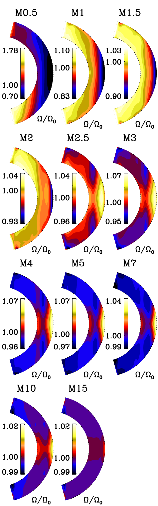
Before we do this in detail, let us look at the differential rotation generated in these simulation by the interplay of rotation and turbulent convection. In Fig. 1, we show the time averaged differential rotation $\Omega=\Omega_{0}+\overline{\mbox{\boldmath$u$}}{}/r\sin\theta$ for all runs. In agreement with earlier findings (Gastine et al. 2014; Käpylä et al. 2014; Fan & Fang 2014; Karak et al. 2015; Viviani et al. 2018), for slow rotation of $\mbox{\rm Co}=0.7$–$2.9$ the equator is rotating slower than the poles, so-called anti-solar differential rotation and for rapid rotation the $\mbox{\rm Co}=3.7$–$40$ the poles are rotating slower than the equator, so-called solar-like differential rotation. The overall relative latitudinal and radial shear is the strongest for the slowest rotation and decreases in the solar-like differential regime for higher rotation rate. This agrees quantitatively with what is found in observation (Reinhold et al. 2013; Lehtinen et al. 2016), with mean-field models (Kitchatinov & Rüdiger 1999) and previous global simulations (e.g. Käpylä et al. 2011; Gastine et al. 2014; Käpylä et al. 2014; Viviani et al. 2018). The difference between the northern and southern hemisphere, for example in Runs M0.5 and M2, is caused by a hemispheric dynamo producing stronger magnetic field in one hemisphere than in the other, see Section 3.1. An interesting feature is the occurrence of a region of a minimum of $\Omega$ at mid-latitude in the solar-like differential rotation regime. This region corresponds to area of large negative shear and has been shown to be responsible for the equatorward migrating dynamo wave in Run M5 (Warnecke et al. 2014, 2016; Käpylä et al. 2017; Warnecke et al. 2018). This region seems to become less pronounced for more rapidly rotating simulations.

Figure 1: Normalized differential rotation $\Omega/\Omega_{0}$ with $\Omega=\Omega_{0}+\overline{\mbox{\boldmath$u$}}{}/r\sin\theta$ for all runs. $\Omega$ has been calculated as a time average over the saturated state.

Figure 2: Mean azimuthal magnetic field $\overline{B}_{\phi}$ as a function of time in years and latitude near the surface ($r=0.98R$) for all runs. The time interval shows the full duration of the saturated state for Runs M0.5 to M3 and an interval of 32 yrs for Runs M4 to M15 to illustrate the similarity in cycle length. The black-white dashed horizontal line indicates the equator.

3.1 Magnetic cycles

Figure 3: Magnetic power spectra for Run M7. (a) Spectra of the mean radial magnetic field $\overline{B}_{r}$ (solid) and the mean azimuthal magnetic field $\overline{B}_{\phi}$ (dashed) near the surface ($r=0.98$; black), in the middle of the convection zone ($r=0.85$; red) and at the bottom of the convection zone ($r=0.72$; blue). (b) Spectra of $\overline{B}{}^{\rm rms}=\sqrt{\overline{B}_{r}{}^{2}+\overline{B}_{\theta}{}^{2}+\overline{B}_{\phi}{}^{2}}$ near the surface ($r=0.85$; red) and averaged over radius (black). All spectra are obtained for each latitude and then averaged. The peaks in a correspond to magnetic cycle periods and in b to activity cycles periods. The solid vertical lines indicate the cycle periods determine from the weighted average of the spectra in a ($P_{\rm cycl}$), the dashed lines indicate the cycle periods determine from the weighted average of the spectra in b ($\tilde{P}_{\rm cycl}$).

Figure 4: Cycle periods as a function of Coriolis number Co showing $P_{\rm cycl}$ in black and $\tilde{P}_{\rm cycl}$ in orange. The green dashed line indicates a power law fit of the Runs M4 to M15.

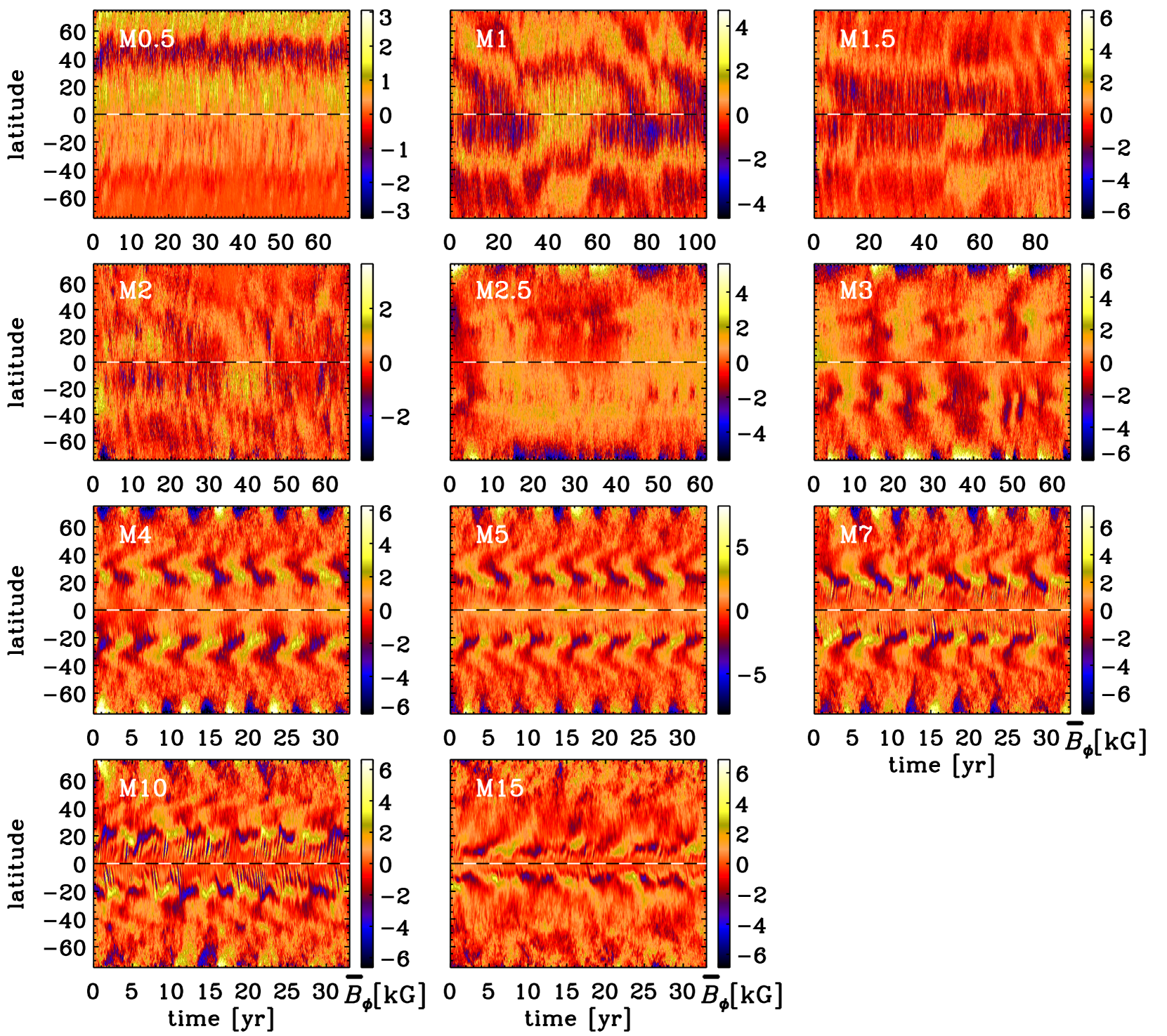
All simulations discussed here show large-scale dynamo action. Lowering the rotation rate below $\tilde{\Omega}=0.5$, produces only a weak large-scale magnetic field ($\tilde{\Omega}=0.4$) or no dynamo action ($\tilde{\Omega}\leq 0.3$) for the same parameters otherwise. A small-scale dynamo is not present in any of these simulations (Warnecke et al. 2018). In Fig. 2, we show the near-surface mean azimuthal magnetic field $\overline{B}_{\phi}$ as function of time and latitude, so-called butterfly diagram for all runs. For the slow rotating Run M0.5, we find the dynamo produces a large-scale magnetic field most pronounced in one hemisphere and with no polarity reversals, only the amplitude shows weak cyclic variations. For Runs M1 to M2.5 the magnetic field is of chaotic nature with polarity reversal, which seems not to be cyclic. This is similar, what have been found before for slowly rotating convective dynamos (Fan & Fang 2014; Karak et al. 2015; Hotta et al. 2016; Käpylä et al. 2017). Interestingly, Run M1 shows some indication of an oscillating magnetic field with anti-solar differential rotation, however, from the current running time, we cannot draw any certain conclusions. Indication of cyclic solution in the anti-solar regime have been also found by Karak et al. (2015), but only recently Viviani et al. (2018) have obtained clear cyclic solutions with many polarity cycles. Run M3 shows indication of a cyclic magnetic field, most pronounced at the poles. The magnetic cycle is even more pronounced in the middle of convection zone, as shown in Warnecke et al. (2016). The Runs M4 to M15 show a clear cyclic magnetic field with regular polarity reversals. The cycle length for these runs seems to be very similar. For Runs M4 to M10 the magnetic field shows a clear equatorward propagation similar what it observed for the solar activity belt. Furthermore, a shorter, much weaker poleward migrating cycle is present in addition to the equatorward migrating mode. It seems to become stronger for increasing rotation. This weak short cycle has been associated with a local $\alpha^{2}$ dynamo mode in addition to the $\alpha\Omega$ dynamo causing the equatorward migration (Käpylä et al. 2016; Warnecke et al. 2018). For Run M15 the field shows indication of both equatorward and poleward migration.

To quantify the cycle period of the magnetic field of all runs, we calculate the power spectrum of the magnetic field and use the strongest peak as the cycle frequency. In the following we distinguish between magnetic cycle and activity cycle. The magnetic cycle includes a full polarity reversal, corresponding to the 22 yrs on the Sun, the activity cycle uses the maximum and minima of the magnetic energy, so 11 yrs for the Sun. We use two ways to calculate our cycle period, for the first we determine the magnetic cycle and take the half and for the second we determine the activity cycle, both results are shown in Table LABEL:runs. For the magnetic cycle we take the radial and azimuthal mean magnetic field component and calculating the power spectrum for each latitude and at three radii ($r=0.98,0.85,72$). Then we average the spectra over latitude to obtain six spectra. Now, we determine the frequency of largest speak of each spectrum with a corresponding error. The error is estimated by taking the full-width-half-maximum unless its narrower than the local grid spacing in the frequency space, in which case we take local grid spacing as an error estimate. From the six frequencies, we calculate the weighted average of the corresponding periods. We take the half of the averaged magnetic cycle period and show it as $P_{\rm cycl}$ with its error $E_{P_{\rm cycl}}$ in Table LABEL:runs.

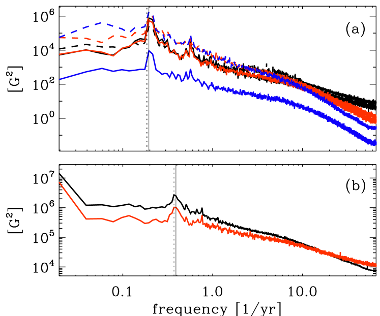
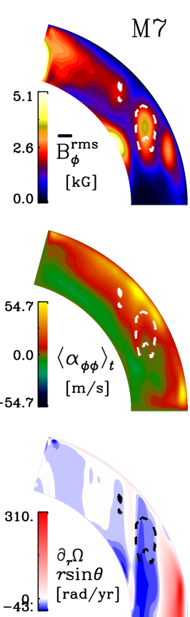
For the activity cycle, we use the root-mean-squared value of the magnetic field $\overline{B}{}^{\rm rms}=\sqrt{\overline{B}_{r}{}^{2}+\overline{B}_{\theta}{}^{2}+\overline{B}_{\phi}{}^{2}}$ near the surface and as a function of radius. As above we calculate the spectrum for each latitude and radius and averaged over them. The cycle period is determined in the same way as for magnetic cycle, without dividing by two. The results are shown as $\tilde{P}_{\rm cycl}$ with its error $\tilde{E}_{P_{\rm cycl}}$ in Table LABEL:runs. In Fig. 3, we show as an example the power spectra of Run M7. Beside the cycle with an activity period of around 2.7 yr, we notice the weak short cycle, which is also visible in Fig. 2.

For the Runs M4 to M15, the cycle periods can be determined well with a small error in $P_{\rm cycl}$. Furthermore, for these Runs $\tilde{P}_{\rm cycl}$ agrees very well with $P_{\rm cycl}$, even though their errors are higher. The larger errors of $\tilde{P}_{\rm cycl}$ are caused by the summation over phase-shifted magnetic field components and this can result in a less pronounced peak in the spectrum of $\overline{B}{}^{\rm rms}$. This can be also seen in the fact that $\tilde{E}_{P_{\rm cycl}}$ is for all runs significant larger than $E_{P_{\rm cycl}}$. For the slowly rotating runs, the periods are not well determined with significant differences with between the two methods and also large errors. In the following, we therefore focus on the analysis of the runs with a clear cycle period.

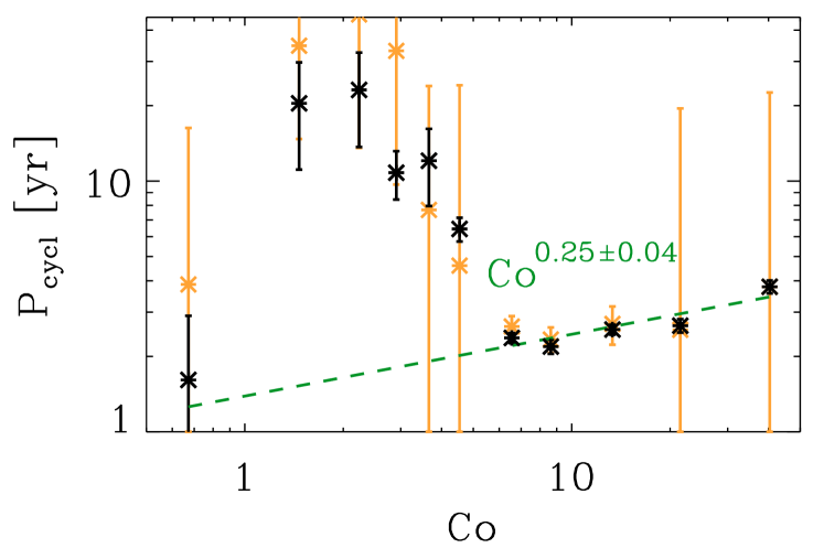
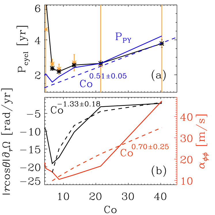
In Fig. 4 we show the cycle periods as a function of Coriolis number. We find two clearly separated group of runs: the slowly rotating simulations with long ill-determined cycles (Runs M1 to M3) and the moderately to rapidly rotating runs with short cycles (Runs M4 to M15). In the latter group the cycle periods increase slightly with increasing rotation. We perform a power law fit for theses runs and obtain $P_{\rm cycl}\propto\mbox{\rm Co}^{0.25\pm 0.04}$, or in terms of rotation period $P_{\rm cycl}\propto P_{\rm rot}^{-0.33\pm 0.05}$. This value is in disagreement with the observation of Noyes et al. (1984b) and Oláh et al. (2016), but agree qualitatively with scaling of advective dominated flux-transport dynamo models (e.g. Dikpati & Charbonneau 1999; Bonanno et al. 2002; Jouve et al. 2010). Strugarek et al. (2017) also found an increase of cycle period with increasing rotation, however their power law fit reveals a much steeper increase with rotation $P_{\rm cycl}\propto P_{\rm rot}^{-1.06}$. The cycle period calculated for Run M5 agrees with the cycle periods obtain for similar runs using the D2 phase dispersion statistics and the Ensemble Empirical Mode Decomposition (Käpylä et al. 2016, 2017).

3.2 Cause of magnetic cycles

Figure 5: Mean magnetic field, $\alpha$ effect and radial shear profiles for Runs M1, M3 and M7. We show the rms mean azimuthal magnetic field averaged over the saturate state $\overline{B}{}_{\phi}^{\rm rms}$ (top row), $\alpha_{\phi\phi}$ determined with the test-field method (middle row) and the radial shear $r\sin\theta\partial\Omega/\partial r$ (bottom row). The dashed lines indicate the region where we calculate $P_{\rm PY}$.

Earlier studies of similar simulations as Run M5 show that the equatorward migrating mean magnetic field can be well explained with a Parker-Yoshimura (Parker 1955; Yoshimura 1975) $\alpha\Omega$-dynamo wave propagating equatorward (Warnecke et al. 2014, 2016, 2018). Following the calculation of Parker (1955) and Yoshimura (1975), we can compute the cycle frequency of the dynamo wave using (see also Stix 1976)

$$\omega_{\rm PY}=\left|\frac{\alpha_{\phi\phi}\,k_{\theta}}{2}r\cos\theta\frac{\partial\Omega}{\partial r}\right|^{1/2},$$ (7)

where $k_{\theta}$ is the latitudinal wave number. The corresponding activity cycle period is then given by

$$P_{\rm PY}={2\pi\over 2\,\omega_{\rm PY}}.$$ (8)

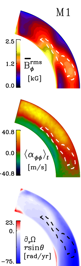
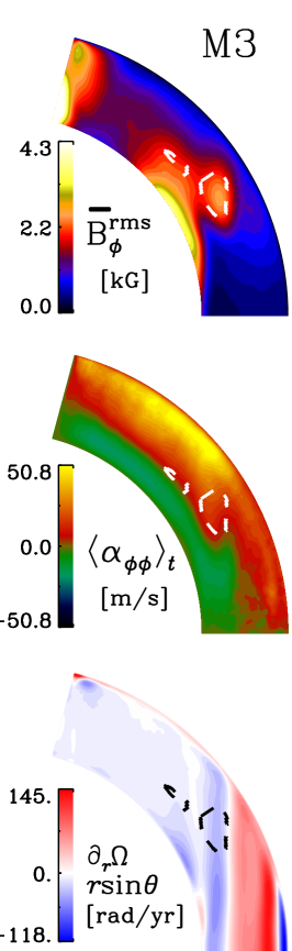
As pointed out by Warnecke et al. (2014), to get a meaningful result for the direction and therefore the period of dynamo wave, the location where measuring the shear and the $\alpha_{\phi\phi}$ is crucial. Following this work, we calculate $P_{\rm PY}$ in the region where i) $\overline{B}{}_{\phi}^{\rm rms}=(\langle\overline{B}{}_{\phi}^{2}\rangle_{t})^{1/2}$ is large, in our case at least larger than the half of the maximum value, ii) the radial shear $\partial\Omega/\partial r$ is negative and iii) $\alpha_{\phi\phi}$ is positive. The last two criteria are needed to excite an equatorward migrating dynamo wave, following the Parker-Yoshimura sign rule. To make sure that these drivers are really responsible to excite a dynamo wave at this location, the production of azimuthal magnetic field must be large at this location, leading to criterion i). The lower limit of half of the maximum value is a reasonable choice; a slightly different value has only little effect on the cycle period determination and on its dependence on rotation rate. The criteria have been also successfully used to confirm Paker-Yoshimura dynamo waves in similar simulations (Warnecke et al. 2014, 2016, 2018; Käpylä et al. 2016). Using these criteria, we then average over these regions. In Fig. 5, we show these regions for Run M1, M3 and M7. To calculate $P_{\rm PY}$, we choose

$$k_{\theta}={1\over R(1-2\Theta_{0}/\pi),}=1.2/R,$$ (9)

where the factor $1-2\Theta_{0}/\pi$ takes into account the absent of the poles in our simulations. However, the actually value of $k_{\theta}$ will only affect the value $P_{\rm PY}$ with a $-1/2$ dependency, but not the scaling with rotation.

In Table LABEL:runs, we list all computed values for $P_{\rm PY}$ in the eleventh column and they agree well with the values of $P_{\rm cycl}$ and $\tilde{P}_{\rm cycl}$ for the runs with well determined cycles (M4 to M15). For oscillatory solution of planetary dynamos, Gastine et al. (2012) found also a good agreement between rotational dependency of measured and dynamo wave predicted cycle length. In Fig. 6a, we show for these runs the cycle periods $P_{\rm cycl}$ and $\tilde{P}_{\rm cycl}$ together with the predicted period $P_{\rm PY}$. A power-law fit results in $P_{\rm PY}\propto\mbox{\rm Co}^{0.51\pm 0.05}$ which is close to $P_{\rm cycl}\propto\mbox{\rm Co}^{0.25\pm 0.04}$. Therefore, the Parker-Yoshimura dynamo wave explains well the weakly dependency of cycle frequency with rotation, we find for the moderately and rapidly rotating simulations. We now go a step further and check, which mechanism of dynamo wave causes this rotational dependency. For this we plot in Fig. 6b the rotational dependency of the radial shear and $\alpha$ effect in terms of $|r\cos\theta|\partial\Omega/\partial r$ and $\alpha_{\phi\phi}$; as for $P_{\rm PY}$ both quantities are averaged over the region of interest. The strength of the shear strongly weakens for larger rotation, with an estimated scaling of $\mbox{\rm Co}^{-1.33\pm 0.18}$. For Run M15 the shear in the region is just below zero explaining the mixture of equatorward and poleward migration pattern shown in Fig. 2. For $\alpha_{\phi\phi}$, we find an increase with rotation corresponding to a scaling of $\mbox{\rm Co}^{0.70\pm 0.25}$, so much less than linear. The strong decrease in shear causes the cycles to become larger with rotation: assuming a constant $\alpha_{\phi\phi}$, shear alone would leading a scaling of $P_{\rm cycl}\propto\mbox{\rm Co}^{0.67\pm 0.09}$. The $\alpha$-effect on the other hand lead to a decrease of cycle length with rotation; $P_{\rm cycl}\propto\mbox{\rm Co}^{-0.35\pm 0.12}$. Because the increase of cycle length due to shear is stronger than the decrease due to the $\alpha$ effect, the resulting cycle length shows only a weak increase with rotation.

Figure 6: (a) Comparison of the cycle periods $P_{\rm cycl}$ (black) and $\tilde{P}_{\rm cycl}$ (orange) with predicted cycle periods using a Parker-Yoshimura dynamo wave $P_{\rm PY}$ (blue) for Runs M4 to M15. The dashed blue line indicates a power law fit to $P_{\rm PY}$. (b) Contributions to the Parker-Yoshimura dynamo wave containing the radial shear (black line; left y-axis) and $\alpha_{\phi\phi}$ (red; right y-axis) for Runs M4 to M15. The dashed lines indicate the corresponding power law fits.

Figure 7: Ratio of rotation period and cycle period $P_{\rm rot}/P_{\rm cycl}$ over the Coriolis number Co. The black asterisks indicate $P_{\rm cycl}$ and the orange ones $\tilde{P}_{\rm cycl}$. The blue solid line shows the predicted cycle length from Equations (7) and (8), the green dashed line the fit of Fig. 4 and the red dashed line a power law fit of Runs M4 to M15.

The surprising issue with interpretation of the magnetic field evolution as a Parker-Yoshimura dynamo wave is that for runs rotating slower than the M4 ($\mbox{\rm Co}=6.5$) it fails. Equation (7) for these runs predict cycle periods of similar length as for the more rapidly rotating runs, but the actual magnetic field shows no clear cyclic evolution. For example, Run M3 shows similar condition for a dynamo wave as in Run M7; there exists a localized region, where the mean toroidal field is strong, $\alpha_{\phi\phi}$ is positive and shear negative, see Fig. 5. In the simulations with anti-solar differential rotation (Run M0.5 to M2), we find instead a more extended region of strong mean toroidal field, positive $\alpha_{\phi\phi}$ and negative shear, however strength of the shear and the $\alpha$ effect should be sufficient to excite an $\alpha\Omega$ dynamo wave. One of the reasons for the absent of an $\alpha\Omega$ dynamo wave can be the larger turbulent magnetic diffusion due to higher convective velocities as shown in Fig. 9. This is in agreement with previous studies of rotating convection in Cartesian boxes (Käpylä et al. 2009). To have a reliable statement, if a $\alpha\Omega$ dynamo is actually operating in these simulation, and what is the reason for not exciting dynamo wave, need to be studied in more detail using all the turbulent transport coefficients. We postpone such a study to the future.

We can now also interpret the scaling of the shear and the $\alpha$ effect in terms of mean-field models (e.g. Krause & Rädler 1980; Rüdiger 1989). From models of differential rotation, one typically finds that the absolute radial and latitudinal differential rotation stays nearly constant for increasing rotation (e.g. Kitchatinov & Rüdiger 1999), which disagrees with our findings. However, we stress here that in these models they take the latitudinal averaged values at bottom and at surface to compute the radial differential rotation, we compute the local radial shear in the region of interest. In mean-field dynamo models $\alpha_{\phi\phi}$ is related to the mean kinetic helicity $\overline{\mbox{\boldmath$u$}{}^{\prime}\mbox{\boldmath$\nabla$}{}\times\mbox{\boldmath$u$}{}^{\prime}}$ and therefore is linear related to the $\Omega$. Taking also the convective turnover time $\tau_{c}$ into account leads to scaling of $\alpha_{\phi\phi}\propto\mbox{\rm Co}$ (e.g. Krause & Rädler 1980). As shown in Warnecke et al. (2018), approximating the diagonal $\alpha$ components with $\alpha_{K}=-1/3\tau_{c}\,\overline{\mbox{\boldmath$u$}{}^{\prime}\mbox{\boldmath$\nabla$}{}\times\mbox{\boldmath$u$}{}^{\prime}}$ is not correct and can lead to the overestimation of $\alpha_{\phi\phi}$. Indeed, we find $\alpha_{\phi\phi}$ in the region of interest depends weaker on rotation as predicted from mean-field models. The overall scaling of $\alpha_{\phi\phi}$ averaged of the simulations might be different, but the import value of $\alpha_{\phi\phi}$ determining the cycle period comes from this region. Warnecke et al. (2018) took also into account the non-linear quenching of the $\alpha$ effect due to magnetic helicity conservation (see Brandenburg & Subramanian 2005, for details) and use the form introduced by Pouquet et al. (1976) $\alpha=-1/3\tau_{c}\,\overline{\mbox{\boldmath$u$}{}^{\prime}\cdot\mbox{\boldmath$\nabla$}{}\times\mbox{\boldmath$u$}{}^{\prime}}+1/3\tau_{c}/\rho\,\overline{\mbox{\boldmath$\nabla$}{}\times\mbox{\boldmath$b$}{}^{\prime}\cdot\mbox{\boldmath$b$}{}^{\prime}}$, but still could not find a agreement with the actual measured $\alpha_{\phi\phi}$, see Fig. 1 and 2 of Warnecke et al. (2018).

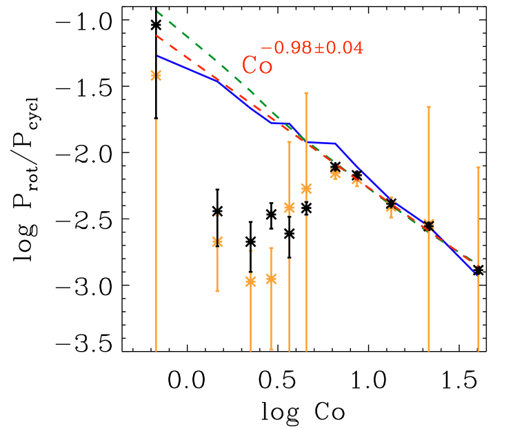
Furthermore, we plot the ratio of rotation period and cycle period $P_{\rm rot}/P_{\rm cycl}$ over Coriolis number, see Fig. 7. We find a scaling of $P_{\rm rot}/P_{\rm cycl}\propto\mbox{\rm Co}^{-0.98\pm 0.04}$ for the runs with well determined cycle. This scaling fits well with the cycle period predicted by a dynamo wave. Interestingly, Run M0.5 fit well to this relation, even though we find no polarity reversals there. In interpretation of stellar observation, $P_{\rm rot}/P_{\rm cycl}$ is often used to determine the quenching of the $\alpha$ effect. If one assumes a linear dependency of $\alpha$ and $\partial\Omega/\partial r$ on $\Omega$ together with Equation (7), $P_{\rm rot}/P_{\rm cycl}$ over Co give an estimate over the rotational quenching of $\alpha$ (e.g. Brandenburg et al. 1998). Moreover, one can go a step further and plot $P_{\rm rot}/P_{\rm cycl}$ over magnetic activity, which is related to the surface magnetic field strengths (e.g. Schrijver et al. 1989). In case of dynamo simulations we can instead use the ratio of magnetic and kinetic energy, so-called dynamo efficiency, to mimic the magnetic activity as done in Fig. 8. Then the $P_{\rm rot}/P_{\rm cycl}$ dependence on magnetic activity can be interpreted as the magnetic quenching of the $\alpha$ effect. However, doing so stellar observations indicate an increase of the $\alpha$ effect with magnetic activity in the inactive and active branch (Brandenburg et al. 1998; Saar & Brandenburg 1999; Brandenburg et al. 2017).

Figure 8: Ratio of rotation period and cycle period $P_{\rm rot}/P_{\rm cycl}$ over magnetic and kinetic energy ratio. The black asterisks indicate $P_{\rm cycl}$ and the orange ones $\tilde{P}_{\rm cycl}$.The red dashed line indicates a power law fit of Run s M4 to M15.

In our simulations, the situation is different. As described above, the radial shear decreases and the $\alpha$ effect increases with higher rotation rate. Therefore, we cannot use $P_{\rm rot}/P_{\rm cycl}$ to estimate the quenching of the $\alpha$ effect. The scaling of $P_{\rm rot}/P_{\rm cycl}\propto\mbox{\rm Co}^{-0.99\pm 0.04}$ as shown in Fig. 7 might seem to be expected, because we plot rotation rate over rotation rate, but the Coriolis number includes also the strength of convection, in terms of $\tau_{c}$, which is influenced by rotation as well. We do not find any indication of branches with positive slopes similar to the inactive or active branch as postulated by Brandenburg et al. (1998). Furthermore, also the slope is different from what is found from the super-active branch, which has a slope of $\mbox{\rm Co}^{-0.43}$ (Saar & Brandenburg 1999).

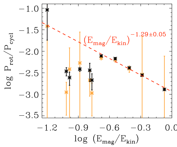
In Fig. 8, we plot $P_{\rm rot}/P_{\rm cycl}$ over ratio of magnetic and kinetic energy, which can be interpreted as the dynamo efficiency, we find a scaling of $P_{\rm rot}/P_{\rm cycl}\propto(E_{\rm mag}/E_{\rm kin})^{-1.29\pm 0.05}$. The scaling seems to agree qualitatively with what is found in Viviani et al. (2018). Also, here, we do not find any indication of a positive slope and therefore a similarity to the activity branches. It seems clear the runs with well determined cycles cannot be interpreted in terms of activity branches with positive slopes. However, our scaling agrees qualitatively with the suggested transitional branch by Distefano et al. (2017).

Figure 9: Turbulent (eddy) magnetic diffusivity over Coriolis number Co. The diffusivity is determined using an estimate of the turbulence in the simulations $\eta_{\rm t}=1/3u_{\rm rms}/k_{\rm f}$ (black) and using the cycle periods as in Equation (12) (red) and as in Equation (13) following Roberts & Stix (1972) (blue). The green dashed line indicates a power law fit of the black asterisk of Runs M4 to M15.

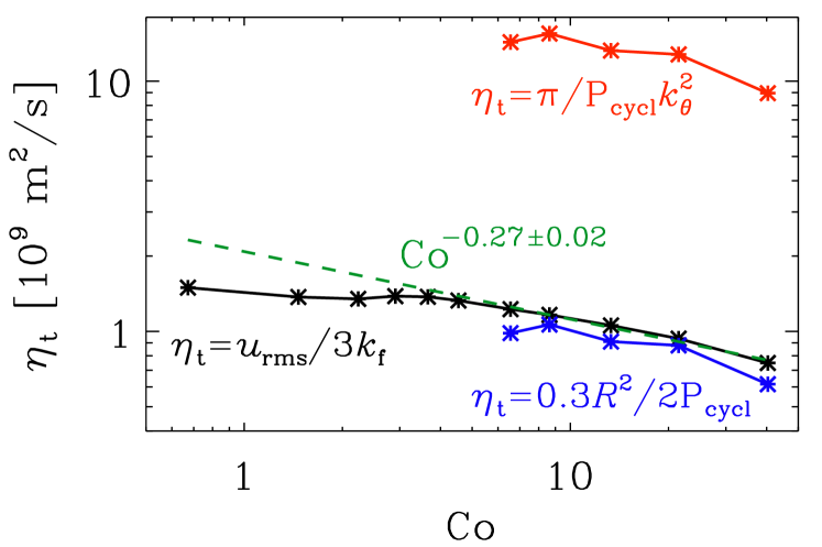
Another way to analyze the scaling of the cycle period with rotation is via the turbulent eddy magnetic diffusivity. In the saturated state the dynamo drivers has to balance to contribution of the magnetic diffusion. In a $\alpha\Omega$ dynamo wave, the balance reads

$$\omega_{\rm PY}-k^{2}\eta_{\rm t}=0,$$ (10)

where $k$ is a wavenumber and $\omega_{\rm PY}$ is given by Equation (7). Therefore, we can use this equation to calculate $\eta_{\rm t}$ based on the cycle frequency and compare with estimated values using the turbulent flow of the simulations. Using the first-oder-smoothing-approximation (FOSA, see e.g. Krause & Rädler 1980) and isotropic and homogeneous turbulence, the turbulent eddy diffusivity can be estimated as

$$\eta_{\rm t}={1\over 3}{u_{\rm rms}\over k_{\rm f}}.$$ (11)

If we assume $k=k_{\theta}$ in Equation (10), we can calculate $\eta_{\rm t}$ based on the cycle period

$$\eta_{\rm t}={2\pi\over 2\,P_{\rm cycl}\,k_{\theta}^{2}}.$$ (12)

Another way is to use the radius $R$ and the depth of the convection zone $0.3R$ of the star to relate $\eta_{\rm t}$ with the cycle period (Roberts & Stix 1972).

$$\eta_{\rm t}={0.3R^{2}\over 2\,P_{\rm cycl}}.$$ (13)

We show the values for both expressions for the runs with well determine cycles (Runs M4 to M15) together with values of Equation (11) as a function of Coriolis number in Fig. 9. $\eta_{\rm t}$ of Equation (13) fits remarkable well with Equation (11). Even the scaling of $\eta_{\rm t}=\mbox{\rm Co}^{-0.27\pm 0.02}$ determined from Equation (11) is the same as expected from the cycle periods $\eta_{\rm t}\propto 1/P_{\rm cycl}\propto\mbox{\rm Co}^{-0.25\pm 0.04}$, see Fig. 4. This good agreement is indeed interesting and not fully expected, because the estimation of $\eta_{\rm t}$ in Equation (11) is based on strong assumptions, which are most likely not fulfilled in these simulations. The values obtained through Equation (12) have obviously the same scaling as Equation (13), however the values are around a factor of 10 higher. This is because of the different values of scales/wave numbers included in this calculation. If we use $k_{\theta}$ instead of $k_{\rm f}$ in Equation (11), the curves would lie closer together. Therefore, the scaling of cycle period with rotation rate of $P_{\rm cycl}\propto\mbox{\rm Co}^{0.25\pm 0.04}$ can also be well explained with the rotational quenching of the turbulent (eddy) magnetic diffusivity.

Figure 10: Ratio of rotation period and cycle period $P_{\rm rot}/P_{\rm cycl}$ over the Coriolis number Co. The black asterisks indicate $P_{\rm cycl}$. The dashed red line indicates the fit $\mbox{\rm Co}^{-0.98}$ of Fig. 7 and the dashed black line the transition from anti-solar to solar like differential rotation. We include the simulations of Viviani et al. (2018) (blue squares, with crosses for wedge runs) and Strugarek et al. (2017) (green diamond), the observational studies of Lehtinen et al. (2016) (purple crosses) and of Brandenburg et al. (2017) (light grey triangles for K dwarfs, dark grey circles for F, G dwarfs, including the Sun: yellow cross).

3.3 Comparison with observational and other numerical studies

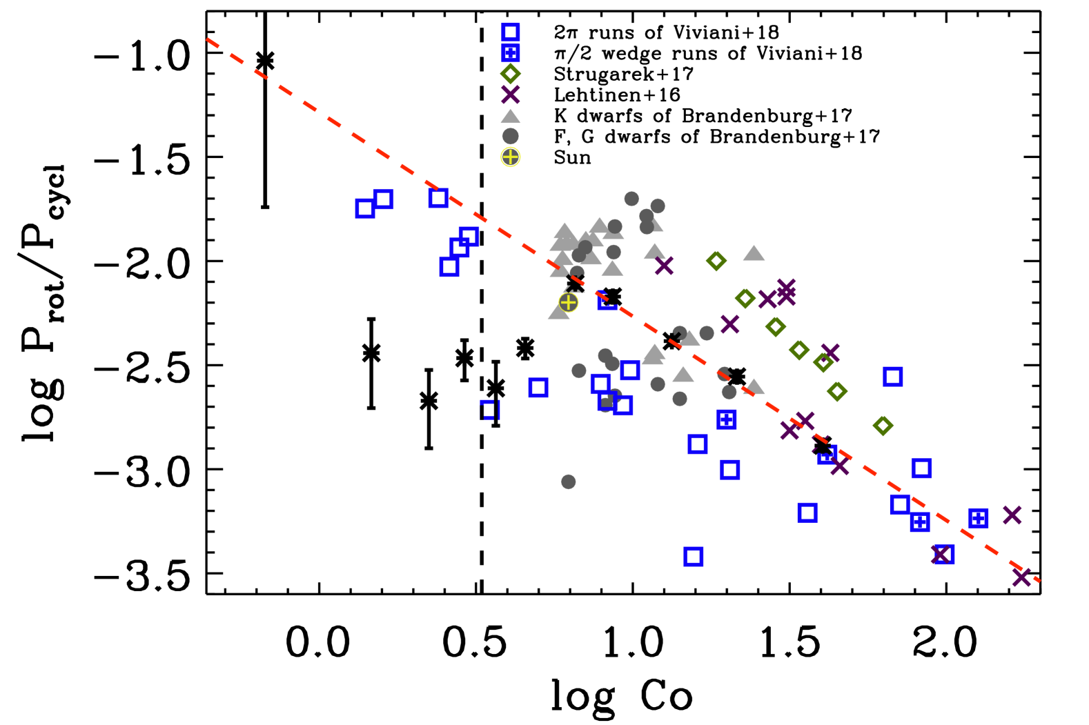
There is only limited amount of numerical studies of cycles of solar and stellar dynamos. In the following, we compare our results with the recent work of Strugarek et al. (2017) and Viviani et al. (2018). The study by Strugarek et al. (2017) include seven models, all showing cyclic dynamo solutions. Even though the authors interpret their models in the vicinity of the Sun, their Rossby numbers indicate a rapid rotational regime. If we convert their numbers to our definition of Coriolis numbers or inverse Rossby number as defined in Brandenburg et al. (1998), respectively, we obtain values of $\mbox{\rm Co}=18$ to $62$. These high numbers are due to their low convective velocities compared to other models (Käpylä et al. 2017). For comparison the estimated Coriolis number of the Sun is $\mbox{\rm Co}=6.2$ (e.g. Brandenburg et al. 2017). In Fig. 10, we plot the models of Strugarek et al. (2017) together with our models. There seems to be no overlap between their and our simulations. However, also their simulations show a decrease of $P_{\rm rot}/P_{\rm cycl}$ with rotation following an even steeper slope. The similar slope might be caused by a similar dynamo mechanism and the small difference and the offset might be because of different system parameters, as Prandtl numbers and/or Reynolds numbers. As shown in Käpylä et al. (2017), the Reynolds numbers in typical simulations with the EULAC code can be lower compared to models of other, similar codes. This might also explain the dominantly axisymmetric large-scale magnetic field solution in Strugarek et al. (2017). The simulations of Viviani et al. (2018) show clearly that if there is a transition from axisymmetric to non-axisymmetric magnetic solution at $\mbox{\rm Co}\geq 3$. However, if the resolution, therefore the Reynolds and Rayleigh numbers, are not high enough, the non-axisymmetric magnetic solution can be not obtained. This is most important for large rotation rates, where the convection is rotationally quenched. Furthermore, Strugarek et al. (2017) claim that their dynamo cycle is caused by a non-linear feedback of the torsional oscillation on the magnetic field. Such an interpretation is not very likely to be correct, because to have a cyclic torsional oscillation one needs a cyclic dynamo in the first place. In the light of the results of this work we are inclined to think that also their cyclic magnetic field is caused by a Parker-Yoshimura dynamo wave. Indeed, their differential rotation profiles show localized regions of strong negative shear, where also the mean magnetic field propagates equatorward.

The study of Viviani et al. (2018) probe a large range of rotation rate in particular in the rapid rotational regime. Their simulations using a similar setup than the one in this work, but for most of their simulations they use a full $2\pi$ extend in the azimuthal direction ($2\pi$ runs) and obtain non-axisymmetric large-scale field solutions for moderately to rapidly rotating runs. In Fig. 10, we also over-plot their simulations. Their $\pi/2$ wedge runs agrees well with our runs and our obtained scaling of $\mbox{\rm Co}^{-0.98\pm 0.04}$. This also means that their estimates of cycle periods based on the temporal variation in the large-scale magnetic energy seems to describe the magnetic cycle well. Their $2\pi$ runs with rapid rotation ($\mbox{\rm Co}\geq 3$) show clearly a different scaling, similar to $\mbox{\rm Co}^{-0.43}$ of the super-active branch (Saar & Brandenburg 1999; Viviani et al. 2018). This might mean that the non-axisymmetric magnetic field solutions have a different scaling than the pure axisymmetric ones. The argument of different scaling is also supported from the fact that the slowly rotating axisymmetric simulations of Viviani et al. (2018) can be well described by the cycle period scaling estimated in this work, see Fig. 10. However, surprising is the fact that for nearly the same rotation rate the $2\pi$ runs show much shorter and much clearer cycles than their corresponding $\pi/2$ wedge simulations.

At the end, we compare our results with observational obtained stellar cycles. One sample comes from Lehtinen et al. (2016), where the authors use photometry to measure cyclic variation is solar-like stars. From this sample, we only plot the cycles which are identified as better than “poor” and plot them in Fig. 10. For rapid rotating stars, their cycles fall surprising well on our scaling relation even though their magnetic field is non-axisymmetric. We note here that Lehtinen et al. (2016) did not do any direct measurement of the magnetic field, but inferred the degree of non-axisymmetry from the spot distributions. For slowly rotation, the stars seems to fall on a parallel line with a similar scaling. Lehtinen et al. (2016) found that the crossover from the transitional branch to the super-active branch happens at around $\mbox{\rm Co}=26.3$ and chromospheric activity value of $\log R^{\prime}_{\rm HK}=-4.4$. We further include the sub-sample of stars from the Mount Wilson sample analyzed by Brandenburg et al. (2017). Our scaling relation falls through these stars; however, a lot of stars are not captured by our scaling. As shown by Brandenburg et al. (2017), the stars around $\mbox{\rm Co}=10$ form the inactive branch with a positive slope and the stars with higher rotation form the active branch also with a positive slope. The active branch is not as confined as the inactive one. In recent works the existence of these branches have been questioned (Reinhold et al. 2017; Distefano et al. 2017). Two new studies of the Mount Wilson sample data (Boro Saikia et al. 2018; Olspert et al. 2017) only find an indication for an inactive branch and otherwise a distribution similar to our scaling showing indication of an transitional branch. There, the authors re-analyses the full Mount Wilson sample, without relying of the cycle determination of Baliunas et al. (1995). The problem with determining cycles from chromospheric and photospheric activity time series is due to the method to for the period search. For star in the inactive branch the cycles are clean and can be well determined, but more active stars with higher rotation rates exhibit a complex behavior with multiple cycles (e.g. Oláh et al. 2016). There, the calculated cycle period can differ depending with method is used (e.g. Olspert et al. 2017). We also note that one to one comparison with observation is not always possible. Even though using the Coriolis number is more meaningful than then the rotational period, because it indicates if the star or simulation is in the slow or rapidly rotating regime, the convective turnover time is usually ill determined for observed stars. Furthermore, as we know the turnover time and therefore the corresponding Coriolis number in the Sun changes several orders of magnitude from the solar surface to the bottom of convection zone (e.g. Stix 2002), it is difficult even for the Sun to estimate a single number as a meaningful Coriolis number. Therefore, Brandenburg et al. (2017) and Olspert et al. (2017) use the chromospheric activity instead of the Coriolis number for their analysis. Using this, Olspert et al. (2017) finds that the cycle periods of this work fit very well with their observed stellar cycles, see their Fig. 6.

Interestingly the cycle data taking from Brandenburg et al. (2017) indicate that the Sun lies close to our scaling relation, actually close to Run M4. If we go a step further and assume the Sun’s 22 yrs magnetic cycle is caused by a Parker-Yoshimura dynamo wave with a cycle-rotation scaling similar to our simulations, we can estimate the corresponding Coriolis number and then with the definition of Equation (5) we also calculate the corresponding value of $u_{\rm rms}$. We calculate a Coriolis number of $\mbox{\rm Co}=8.5$ corresponding to $u_{\rm rms}=21.5\,{\rm m/s}$. This velocity would be located at around $160\,{\rm Mm}$ depth ($r=0.78\,R$) according to the mixing length model of Spruit (1974) or $r=0.72\,R$ for the model of Stix (2002). Therefore, this kind of dynamo wave cannot be driven by the near-surface shear layer, it must instead be driven by a positive radial shear and an inversion of sign of $\alpha_{\phi\phi}$ in the deeper part of the convection zone to get an equatorward migrating magnetic field (Duarte et al. 2016).

4 Conclusions

We use 3D MHD global dynamo simulations to investigate the rotational dependency of magnetic activity cycles. For moderately and rapidly rotating runs ($\mbox{\rm Co}\geq 6.5$), we find well-defined cycles in range between 2 to 4 yrs. For slowly rotating runs, we find irregular cycles with mostly longer periods. There the cycle periods can be only ill-determined. Using the $\phi\phi$ component of the $\alpha$ tensor measured with the test-field method, and the radial shear we find a good agreement of the cycle period predicted by a Parker-Yoshimura dynamo wave for moderately to rapid rotating runs. There we find that the cycle period only weakly depends on rotation ($P_{\rm cycl}\propto\mbox{\rm Co}^{0.25\pm 0.04}$ and $P_{\rm cycl}\propto P_{\rm rot}^{-0.33\pm 0.05}$). Also this scaling is well reproduced by a Parker-Yoshimura dynamo wave. $\alpha_{\phi\phi}$ increases only weakly with rotation ($\alpha_{\phi\phi}\propto\mbox{\rm Co}^{0.70\pm 0.25}$) and the strength of negative radial shear decreases larger than linear with rotation $\partial\Omega/\partial r\propto\mbox{\rm Co}^{-1.33\pm 0.18}$. This is not in agreement with mean-field theory, where $\alpha$ depends linear on the rotation (e.g. Krause & Rädler 1980). Also from models of differential rotation ones finds the radial shear has not a strong dependency on rotation (Kitchatinov & Rüdiger 1999). However, these models usually look at the global quantities and we determine our scaling from localized region responsible for driving the dynamo wave.

Looking at the ratio of rotation and cycle period over Coriolis number, we do not find any indication of activity branches with positive slopes as found from observation of stellar cycles by Brandenburg et al. (1998) and Saar & Brandenburg (1999). The negative slope of our simulations with well determined cycles seems to be more in agreement with the transitional branch postulated by Distefano et al. (2017) and confirmed by Boro Saikia et al. (2018) and Olspert et al. (2017). Furthermore, our results suggest that the cyclic magnetic fields found in the work by Strugarek et al. (2017) are also caused by a Parker-Yoshimura dynamo wave, because indeed their simulations produce strong negative shear in the location, where the magnetic field is oscillating. By assuming the solar magnetic cycle is caused by a Parker-Yoshimura dynamo wave following a similar scaling as in our simulations, we can conclude that the dynamo in the Sun operates near the bottom of convection zone, where turbulent velocities are around $20\,{\rm m/s}$.

The cycle period dependence on rotation of our simulations can be also well explained via the rotational quenching of the turbulent diffusivity, which contribution has to balance with the dynamo driver in the saturated stage. We find the nearly the same scaling for the turbulent eddy diffusivity with Coriolis number as expected from a direct inverse proportionality of the diffusivity with cycle period (e.g. Roberts & Stix 1972).

For the slowly rotating runs a Parker-Yoshimura dynamo wave seems to be not excited, as the predicted periods do not fit with the measured ones. This might be due to a higher turbulent diffusion in this rotation regime as found in Käpylä et al. (2009). In particular, these simulations need to be further investigated using the full set of turbulent transport coefficients. Moreover, we note here that in the rapidly rotating regime the magnetic field can become highly non-axisymmetric as found recently in observations (e.g. Lehtinen et al. 2016) and simulations (Viviani et al. 2018). The work of Viviani et al. (2018) indicate a weaker scaling of $P_{\rm rot}/P_{\rm cycl}$ with Coriolis number than what we find in our work and this might be due to the non-axisymmetric magnetic field solution, which are suppressed in our work because of the wedge assumption.

We stress here that the cycles determined from our simulation are directly linked to the magnetic field. Observational stellar cycles are mostly measured from chromospheric activity variations (Ca II H&K) or photometry. These are only proxies of the magnetic field strength and might not capture all the features of cyclic variations. Therefore, it would be useful to determine also the integrated variability caused by the simulated magnetic cycles. Furthermore, we will in future also investigate how coronal heating and therefore the X-ray luminosity will depend on the cyclic magnetic field. For this it is crucial to combine convective dynamo models with a coronal envelope as done in Warnecke et al. (2011, 2012, 2013, 2016). This is in particular important to study the role of helicity connecting the dynamo active stellar convection zones with stellar coronae, as the magnetic helicity might play an important role in the heating of coronae (Warnecke et al. 2017).