The asymmetry of sunspot cycles and Waldmeier relations as due to nonlinear surface-shear shaped dynamo

Abstract

The paper presents a study of a solar dynamo model operating in the bulk of the convection zone with the toroidal magnetic field flux concentrated in the subsurface rotational shear layer. We explore how this type of dynamo may depend on spatial variations of turbulent parameters and on the differential rotation near the surface. The mean-field dynamo model takes into account the evolution of magnetic helicity and describes its nonlinear feedback on the generation of large-scale magnetic field by the $\alpha$-effect. We compare the magnetic cycle characteristics predicted by the model, including the cycle asymmetry (associated with the growth and decay times) and the duration - amplitude relation (Waldmeier’s effects), with the observed sunspot cycle properties. We show that the model qualitatively reproduces the basic properties of the solar cycles.

1 Introduction

The sunspot’s activity is organized on large scales, forming the Maunder butterfly diagram. It is believed to represent the time - latitude pattern of the large-scale toroidal magnetic field generated in the convection zone. Another component of the solar activity is represented by the global poloidal magnetic field extending outside the Sun and shaping the solar corona. Both components synchronously evolve as the solar 11-year cycle progresses. The global poloidal field reverses the sign in the polar regions near the time of maxima of sunspot activity. Most of the current solar dynamo models suggest that the toroidal magnetic field that emerges on the surface and forms sunspots is generated near the bottom of the convection zone, in the tachocline or just beneath it in a convection overshoot layer (see, e.g., Ruediger & Brandenburg, 1995; Choudhuri et al., 1995; Tobias & Weiss, 2007; Parker, 1993). The belief in a deep-seated solar dynamo comes from the fact that this region is sufficiently stable to store magnetic flux despite the magnetic flux-tube buoyancy effect. However, observations of rotation rates of emerging magnetic flux within the latitude bands $\pm 30^{\circ}$ support a concept of relatively shallow sunspots (Benevolenskaya et al., 1999) possibly rooted within the subsurface rotational shear layer. This concept has support from local helioseismology as well (Birch, 2011) .

There are further theoretical arguments that the subsurface angular velocity shear can play an important role in the dynamo process distributed in the convection zone (Brandenburg, 2005). In our previous paper (Pipin & Kosovichev, 2011) (PK11) we proposed a model of a subsurface-shear shaped solar $\alpha\Omega$ dynamo. Our model shows that allowing the large-scale toroidal magnetic field to penetrate into the surface layers of the Sun changes the direction of the latitudinal migration of the toroidal field belts and produces the magnetic butterfly diagram in a good qualitative agreement with the solar cycle observations. The dynamo wave penetrates close to the surface and propagates along iso-surfaces of the angular velocity in the subsurface rotational shear layer in agreement with the Parker-Yoshimura rule (Yoshimura, 1975). The standard boundary condition typically used in dynamo theories is to match the internal solution to the potential magnetic field extending outside of the dynamo region. This boundary condition does not allow to the toroidal component to penetrate to the surface.

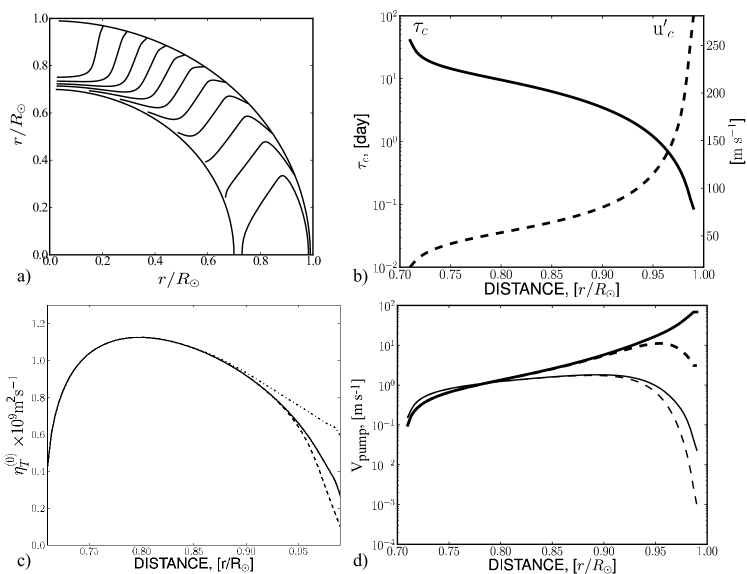
Figure 1: Parameters of the solar convection zone: a) contours of the constant angular velocity plotted in the range $(0.75-1.05)\Omega_{0}$ with a step of $0.025\Omega_{0}$, $\Omega_{0}=2.86\cdot 10^{-7}s^{-1}$; b) turnover convection time $\tau_{c}$, and the RMS convective velocity $u^{\prime}_{c}$; c) the background turbulent diffusivity $\eta_{T}^{(0)}$ profiles; the solid curve shows the profile of the Stix(2002) model; the dashed and dotted curves show models with the reduced and increased sub-surface diffusivities discussed in Sec. 3.1; d) the radial (thick lines) and the latitudinal (thin lines) turbulent pumping velocities at $\theta=45^{\circ}$ for models P1 (solid curves) and P2 (dashed curves), see Table 1;

In our previous model the penetration of toroidal magnetic fields to the surface was modeled by a special boundary condition at the top of the dynamo region. This boundary condition was formulated as a linear combination of vacuum (potential field) and perfectly conducting plasma conditions. The perfectly conducting part results in an increase of the toroidal component of the large-scale magnetic field at the boundary. Such boundary condition, used in PK11, models a partial penetration of the toroidal field into the solar atmosphere, but from the physical point of view such formulation is rather artificial. The penetration to the surface can be modeled more physically by extending the computational domain close to the surface and using the magnetic diffusivity profile that follows from the standard solar interior model. This diffusivity decreases toward to the surface and results in increasing of the toroidal magnetic field in that direction (and an increase of the gradient of the toroidal magnetic field as well). The decrease of the turbulent diffusivity, $\eta_{T}\sim{\displaystyle\frac{1}{3}}u^{\prime}\ell$, (where $u^{\prime}$ is the convective RMS velocity and $\ell$ is the mixing length) is predicted by the mixing-length theory of the solar interior. This motivates us to extend the integration domain from $(0.71\div 0.97)R_{\odot}$, used in PK11, to $(0.71\div 0.99)R_{\odot}$. The convection model of Stix (2002) predicts that towards to the surface the mixing-length, $\ell$, decreases much faster than $u^{\prime}$ increases. Figure 1c shows the radial profile of the turbulent diffusivity in the convection zone model. In this paper we study how the sharp decrease of the magnetic diffusivity influences the strength and distribution of the toroidal field in the upper layers of the convection zone.

There is another reason for extending the integration domain closer to the surface. In the near surface layers the density stratification gradient is very strong compared to the bulk of the convection zone. The mean-field theory predicts a downward turbulent drift of the large-scale magnetic filed in the presence of the density stratification gradient (Kitchatinov, 1991) (similar results were obtained by Pipin, 2008). The effective downward drift of large-scale magnetic field results from magnetic fluctuations in the stratified turbulence. It can be interpreted as follows (see Kitchatinov, 1991). The intensity of the magnetic fluctuations $\overline{b^{2}}=\mu_{0}\bar{\rho}\overline{u^{\prime 2}}$ ($\overline{\rho}$ is the mean density) rises in the direction of the density gradient because the turbulent RMS velocity varies slower than $\overline{\rho}$. Random Lorenz forces, which are induced by small-scale magnetic fields $\mathbf{b}$ and large-scale field $\overline{\mathbf{B}}$, produce fluctuating flows $\mathbf{u}^{\prime}\approx{\displaystyle\frac{\mathbf{\left(\nabla\times\mathbf{b}\right)}\times\overline{\mathbf{B}}}{\mu\overline{\rho}}\tau_{c}}$. The resulted electromotive force $\overline{\mathbf{u}^{\prime}\times\mathbf{b}}$ is perpendicular to the large-scale field. This can be interpreted as an effective downward velocity drift of the large-scale magnetic field (Kitchatinov, 1991). The theory also predicts that this kind of turbulent pumping is quenched by the influence of the Coriolis force, which results in the velocity of the effective drift to be greatest near the surface where the density stratification is strong. Thus, qualitatively, this effect works similarly to so-called “topological pumping” (Drobyshevski & Yuferev, 1974) .

Our study includes an equation of the magnetic helicity evolution, proposed by Kleeorin & Ruzmaikin (1982) and Kleeorin & Rogachevskii (1999). This equation describes the balance between the small-scale turbulent magnetic helicity and the large-scale magnetic helicity generated by the dynamo process, and has been used in many previous dynamo studies (e.g., Brandenburg & Subramanian (2005) and references therein). One of our goals is to explore nonlinear feedback of the magnetic helicity on the basic properties of sunspot cycles, e.g., the relationship between the rise and decay times, and between the length and strength of the cycles. The results for a dynamo model in a single-mode approximation (Kitiashvili & Kosovichev, 2009, 2010) have suggested the importance of the nonlinear magnetic helicity effects for the solar-cycle behavior. The next section describes the formulation of the 2D mean-field dynamo model, including the basic assumptions, the reference model of the solar convection zone, and input parameters of the large-scale flows. Section 3 presents the results and discussion. The main findings are discussed in Section 4.

2 Basic equations

The dynamo model is based on the standard mean-field induction equation in perfectly conductive media (Krause and Rädler, 1980):

$$\frac{\partial\mathbf{B}}{\partial t}=\boldsymbol{\nabla}\times\left(\mathbf{\boldsymbol{\mathcal{E}}+}\mathbf{U}\times\mathbf{B}\right)$$

where $\boldsymbol{\mathcal{E}}=\overline{\mathbf{u\times b}}$ is the mean electromotive force, with $\mathbf{u,\,b}$ being the turbulent fluctuating velocity and magnetic field respectively; $\mathbf{U}$ is the mean velocity. General expression for $\boldsymbol{\mathcal{E}}$ was obtained by Pipin (2008) (hereafter P08). Following Krause and Rädler(1980) we write the expression for the mean electromotive force as follows:

$$\mathcal{E}_{i}=\left(\alpha_{ij}+\gamma_{ij}\right)\overline{B}_{j}-\eta_{ijk}\nabla_{j}\overline{B}_{k}.$$ (1)

Tensor $\alpha_{i,j}$ represents the alpha effect, including the hydrodynamic and magnetic helicity contributions, $\alpha_{ij}=C_{\alpha}\psi_{\alpha}(\beta)\sin^{2}\theta\alpha_{ij}^{(H)}+\alpha_{ij}^{(M)},$ where the hydrodynamical part of the $\alpha$-effect, $\alpha_{ij}^{(H)}$, and the quenching function, $\psi_{\alpha}$, are given in Appendix (see also in Pipin & Kosovichev, 2011), the parameter $C_{\alpha}$ controls the amplitude of the $\alpha$-effect. The hydrodynamic $\alpha$-effect term is multiplied by $\sin^{2}\theta$ ($\theta$ is colatitude) to prevent the turbulent generation of magnetic field at the poles. The contribution of the small-scale magnetic helicity $\overline{\chi}=\overline{\mathbf{a\cdot}\mathbf{b}}$ ($\mathbf{a}$ is a fluctuating vector-potential of magnetic field) to the $\alpha$-effect is defined as $\alpha_{ij}^{(M)}=C_{ij}^{(\chi)}\overline{\chi}$ , where coefficient $C_{ij}^{(\chi)}$ depends on the turbulent properties and rotation, and is given in Appendix. The other parts of Eq.(1) represent the effects of turbulent pumping, $\gamma_{ij}$, and turbulent diffusion, $\eta_{ijk}$. They are the same as in PK11. We describe them in Appendix.

The nonlinear feedback of the large-scale magnetic field to the $\alpha$-effect is described as a combination of an "algebraic" quenching by function $\psi_{\alpha}\left(\beta\right)$ (see Appendix and PK11), and a dynamical quenching due to the magnetic helicity conservation constraint. The magnetic helicity, $\overline{\chi}$ , subject to a conservation law, is described by the following anzatz (Kleeorin & Ruzmaikin, 1982; Kleeorin & Rogachevskii, 1999):

$$\frac{\partial\overline{\chi}}{\partial t} = -2\left(\boldsymbol{\mathcal{E}\cdot}\overline{\mathbf{B}}\right)-\frac{\overline{\chi}}{R_{\chi}\tau_{c}},$$ (2)

where $\tau_{c}$ is a typical convection turnover time. Parameter $R_{\chi}$ controls the helicity dissipation rate without specifying the nature of the loss. Generally, we can expect that the formulation of the the helicity loss term in Eq.(2) affects properties of the dynamo solutions. This is suggested by results that can be found in the literature (Brandenburg et al., 2007; Mitra et al., 2010; Guerrero et al., 2010; Mitra et al., 2011). The physics of helicity loss is poorly understood, and influence the various processes of the helicity flux loss on the properties of magnetic cycles deserves a separate study. To reduce the number of free parameters in the model we consider the simplest form of helicity flux loss. The parameter $R_{\chi}$ controls the amount of the magnetic flux generated by the dynamo. This amount can be roughly estimated from observations. We use the range of $R_{\chi}$ that gives the total magnetic flux of the order of $\approx 10^{24}-10^{25}$ Mx in agreement with observations (Schrijver & Harvey, 1994). Another parameter controlling the helicity dissipation in our model is $\tau_{c}$. It is given by the solar interior model. It seems to be reasonable that the helicity dissipation is most efficient in the near surface layers because of the strong decrease of $\tau_{c}$ (see Figure 1b).

We use the solar convection zone model computed by Stix (2002), in which the mixing-length is defined as $\ell=\alpha_{MLT}\left|\Lambda^{(p)}\right|^{-1}$, where $\mathbf{\boldsymbol{\Lambda}}^{(p)}=\boldsymbol{\nabla}\log\overline{p}\,$ is the pressure variation scale, and $\alpha_{MLT}=2$. The turbulent diffusivity is parametrized in the form, $\eta_{T}=C_{\eta}\eta_{T}^{(0)}$, where $\eta_{T}^{(0)}={\displaystyle\frac{u^{\prime}\ell}{3}}$ is the characteristic mixing-length turbulent diffusivity, $\ell$ and $u^{\prime}$ are the typical correlation length and RMS convective velocity of turbulent flows, respectively and $C_{\eta}$ is a constant to control the intensity of turbulent mixing. In the paper we use $C_{\eta}=0.05$. The differential rotation profile, $\Omega=\Omega_{0}f_{\Omega}\left(x,\mu\right)$, $x=r/R_{\odot}$, $\mu=\cos\theta$ is a modified version of an analytical approximation to helioseismology data, proposed by Antia et al. (1998), see Figure 1a.

We use the standard boundary conditions to match the potential field outside and the perfect conductivity at the bottom boundary. As discussed above, the penetration of the toroidal magnetic field in to the near surface layers is controlled by the turbulent diffusivity and pumping effect (see Figures 1c and 1d).

Model	$C_{\alpha}$	$R_{\chi}$	${\displaystyle\frac{\left.\eta_{T}\right|_{0.99R_{\odot}}}{\max(\eta_{T})}}$	$r\boldsymbol{\Lambda}_{min}^{(\rho)}$	$\left\langle\!B_{\phi}\!\right\rangle_{SL}$, G	$B_{r}^{Polar}$, G	$A_{W}$	Period, Yr
P1 P2 P3	0.03	-	0.245	-160 -30 0	1000 450 60	7.2 3.5 0.15	0.74 0.94 0.89	13.4 11.4 8.6
D1 D2	0.03	-	0.645 0.091	-160	450 1600	3.6 14.4	0.78 0.68	10.7 15.2
CQ1 CQ2 CQ3	0.03	$5\!\cdot\!10^{4}$ $10^{3}$ $10^{2}$	0.245	-160	- 66 152	- 0.3 3.6	- 0.71 0.59	- 11.74 11.17
WR1	0.03,0.04 0.05,0.06	50	0.245	-160	203,294 351,396	1.1,1.8 2.3,2.6	0.68,0.54 0.5,0.42	11.35,10.60 10.15,9.67
WR2	0.03,0.04 0.05,0.06	100	0.245	-160	152,220 266,302	0.8,1.3 1.8,2.0	0.59,0.53 0.49,0.39	11.17,10.44 9.80,9.33
WR3	0.03,0.04 0.05,0.06	200	0.245	-160	102,150 182,206	0.5,0.9 1.2,1.4	0.57,0.50 0.44,0.38	11.10,10.40 9.80,9.27

Table 1: Parameters and characteristics of the dynamo models: the $\alpha$-effect parameter $C_{\alpha}$; parameter $R_{\chi}$ controls the helicity dissipation rate; ${\displaystyle\frac{\left.\eta_{T}\right|_{0.99R_{\odot}}}{\max(\eta_{T})}}$ is the ratio between the maximum background turbulent diffusivity and the value at the top boundary (in the reference model of Stix (2002) this value is 0.245); $r\boldsymbol{\Lambda}_{min}^{(\rho)}$ is the minimum of the density gradient height at the top; $\left\langle B_{\phi}\right\rangle_{SL}$ is the maximum strength of the toroidal magnetic field averaged in the range of $0.95-0.99R_{\odot}$; $B_{r}^{Polar}$ is the maximum strength of the radial polar magnetic field at $0.99R_{\odot}$; $C_{W}$ is a calibration coefficient used for calculation of the sunspot number parameter; $A_{W}$ is the sunspot number asymmetry parameter obtained in the models; Period is the period of sunspot cycles from the dynamo models.

3 Results

We summarize the parameters and characteristics of the dynamo models in Table 1. For simulating the sunspot number obtained from solar observations we use the relation suggested by Bracewell (1988):

$$W(t)=C_{W}\,\max\left(\left|\left\langle B(r,\theta,t)\right\rangle_{0.95-0.99R}\right|,0<\theta<180\right)^{3/2}$$ (3)

where $B$ is the toroidal magnetic field strength and $C_{W}$ is the calibration coefficient, we use $C_{W}=1/40$. We define the asymmetry parameter of the cycle as the ratio between the modulus of the mean decay rate and mean rise rate, $A_{W}={\displaystyle\frac{\overline{\partial_{t}W}\biggr{|}_{\partial_{t}W>0}}{\left|\overline{\partial_{t}W}\right|\biggr{|}_{\partial_{t}W<0}}}$. The simulations were started from initial states with zero toroidal magnetic field and weak poloidal field which is symmetric about the equator. The solution is found by a semi-implicit method using a finite-difference approximation in radius and a pseudospectral decompisition in terms of Legendre polynomials in latitude. The numerical scheme conserves the parity of solution with respect to the equator. The characteristics of the dynamo models were determined from the stationary periodic solutions.

3.1 Effects of the near surface diffusion and turbulent pumping

In this part of the paper we fix the $\alpha$-effect parameter $C_{\alpha}=0.03$ (the dynamo instability threshold is $C_{\alpha}\approx 0.02$ ). In the near surface layers the Coriolis number is rather small. Therefore, the turbulent pumping primarily depends on the density gradient $\boldsymbol{\Lambda}^{(\rho)}$ and diffusion coefficient $\eta_{T}$. The gradient parameter $r\boldsymbol{\Lambda}^{(\rho)}$ varies from $\approx-7$ at $r=0.71R_{\odot}$ to $\approx-160$ at $r=0.99R_{\odot}$. To illustrate the influence of the pumping effect on the dynamo model solution we examine three different cases (P1, P2 and P3 in Table 1). Model P1 employs the density gradient profile provided by the Stix (2002) model. In model P2, we introduce an artificial limit on the level of $r\Lambda^{(\rho)}=-30$ suggested by Kitchatinov et al. (2000). In model P3, we completely neglect the pumping effect. Profiles of the radial and the latitudinal pumping velocities at $\theta=45^{\circ}$ for models P1 and P2 are shown in Figure 1d. Note, that compared to the plotted values the amplitude of the velocities in the models is reduced by factor $C_{\eta}=0.05$.

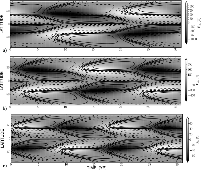
Figure 2: Illustration of the influence of the magnetic pumping effect (models P1, P2 and P3 in Table 1). Time-latitude diagrams of the toroidal magnetic field averaged over the depth range $0.95-0.99R_{\odot}$ (gray scale) and the radial field at $r=0.99R_{\odot}$(shown by contours), for three cases of turbulent pumping: a) model P1 : the density gradient profile provided by the Stix (2002) model, the radial field varies in range $\pm 21$G; b) model P2: the density gradient effect is restricted as suggested by Kitchatinov et al. (2000), the radial field varies in range $\pm 14.5$ G; c) model P3: the pumping effect due to the density gradient is neglected, the radial field varies in range $\pm 1.4$G.

The time - latitude toroidal magnetic field “butterfly” diagrams, which were averaged over the depths from $r=0.95R_{\odot}$ to $r=0.99R_{\odot}$, and the radial magnetic field evolution at $r=0.99R_{\odot}$ for models P1, P2 and P3 are shown in Figures 2. We find that the larger amplitude of the downward turbulent pumping results in the greater strength of the near surface toroidal magnetic field. The turbulent pumping increases the efficiency of the subsurface shear generation effect. This leads to a faster migration rate of the toroidal magnetic field to the equator (see, Yoshimura, 1975).

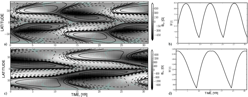
Figure 3: Left column, the same as in Figure 2 for the larger (top) and smaller (bottom) sub-surface turbulent diffusivity, models D1 and D2 respectively. Right column - the simulated sunspot number, see definition in the text.

A similar effect can be produced by changing the turbulent diffusivity profile near the surface. In Figure 3 we show the results for two cases of the increased (D1) and decreased (D2) turbulent diffusivity (Figure 1c). The diagrams for these two cases can be compared with the reference Stix’s model P1 in Figure 2a. The smaller the surface turbulent diffusivity level, the greater toroidal magnetic field strength. In the reference case the typical magnetic field strength is $\sim 1$ kG. If the surface turbulent diffusivity is three time smaller the field strength increases to $\sim 1.6$ kG; if the diffusivity is two time larger, then the field strength is only about $\sim 450$ G. The inclination of the toroidal field patterns migrating toward the equator (latitudinal migration speed) does not change considerably with the changes of the turbulent diffusivity profile. However, when the surface turbulent diffusivity is smaller, the toroidal magnetic field migrates closer to the equator, and the cycle becomes longer.

For simulating the sunspot number obtained from solar observations we use the relation motivated by Bracewell (1988), see Eq.(3). The estimated sunspot number for the models with the increased and decreased sub-surface turbulent diffusivity is shown in Figure 3 (left panels). The asymmetry between the rise and decay phases is clearly seen for the model with the decreased surface turbulent diffusivity. In the mean-field dynamo concept the decay phase of the large-scale toroidal magnetic field is defined by turbulent diffusion (Parker, 1979). The decrease of the surface turbulent diffusivity increases the decay time when the toroidal field is located closer to the surface.

3.2 Magnetic helicity effect and the Waldmeier’s relations

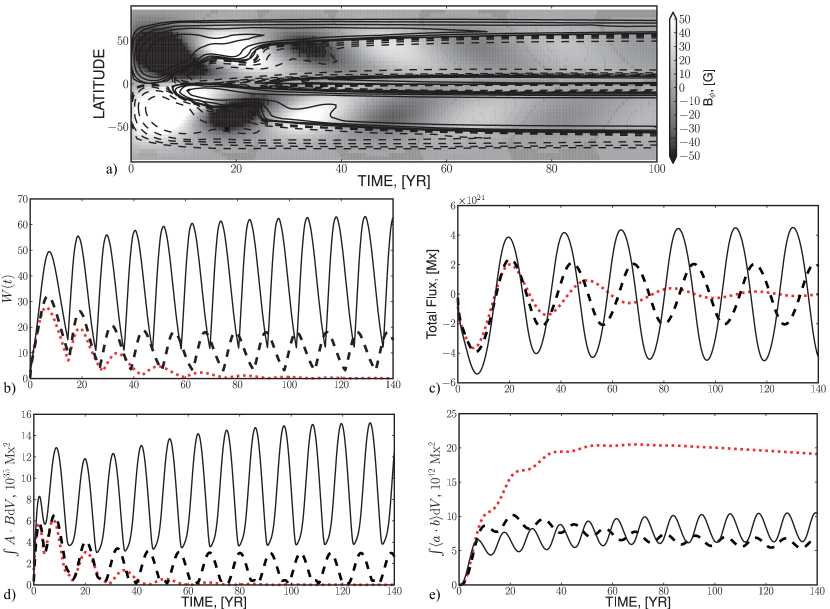
Figure 4: Illustration of the dynamo models with the catastrophic quenching (model CQ1) and without it (models CQ2 and CQ3): a) toroidal field (gray scale) and current helicity (contours, in range $\pm 3\ 10^{-5}$ G²m^-1) for model CQ1; evolution of global characteristics: b) the sunspot number parameter W, c) the total magnetic flux, d) total large-scale magnetic helicity; e) total small-scale magnetic helicity for models CQ1(dots), CQ2(dashed curves), CQ3(solid curves).

The evolution of magnetic helicity based on the conservation law is described by Eq.(2). Without helicity fluxes from the dynamo domain (Kleeorin et al., 2000; Vishniac & Cho, 2001) or in absence of helicity dissipation, the generation of magnetic helicity by dynamo leads to “catastrophic quenching” of the $\alpha$-effect, which stops the dynamo process (see, e.g., Vainshtein & Cattaneo, 1992; Kleeorin et al., 2000; Brandenburg & Subramanian, 2005). In our model the dissipation of magnetic helicity is described by a decay term:${\displaystyle-\frac{\overline{\chi}}{R_{\chi}\tau_{c}}}$. We illustrate the catastrophic quenching in dynamo model CQ1 in Figure 4, which shows the results for $R_{\chi}=5\times 10^{4}$. In this case, the rate of the helicity loss from the Sun is small, and the dynamo process stops after 3-4 periods (2 magnetic cycles). The time-latitude diagram for the current helicity, which is estimated as $h_{\mathcal{C}}=\overline{\mathbf{b\cdot}\boldsymbol{\nabla}\times\mathbf{b}}\approx\overline{\chi}/\ell^{2}$, is shown together with the magnetic butterfly diagram. We see that the total magnetic helicity generated by the dynamo is decaying much slower than the dynamo waves. Figure 4 also shows the evolution of the sunspot parameter, the total magnetic flux, the total turbulent magnetic helicity and total large-scale magnetic helicity. For comparison with case $R_{\chi}=5\times 10^{4}$ (model CQ1), we show the results for $R_{\chi}=10^{3},\,10^{2}$ (models CQ2 and CQ3). In the case of $R_{\chi}=10^{3}$ (model CQ2) the dynamo is stabilized at a quite low level with the maximum toroidal magnetic field strength of about $50\,\mathrm{G}$ and the total magnetic flux of about $10^{24}$ Mx. For the high dissipation rate of the magnetic helicity, $R_{\chi}=10^{2}$, (model CQ3) the maximum of the toroidal magnetic field strength inside the convection zone is about $450\,\mathrm{G}$, and in the surface layer it reaches about $150\,\mathrm{G}$. In model CQ3, the total magnetic flux is about $4\times 10^{24}$ Mx. This roughly agrees with observational results of Schrijver & Harvey (1994). Taking into account the results shown in Figure 4d we can estimate the amount of the helicity loss from the Sun per cycle. In the model CQ3 it is about $1.26\times 10^{45}\,\mathrm{Mx^{2}}$.

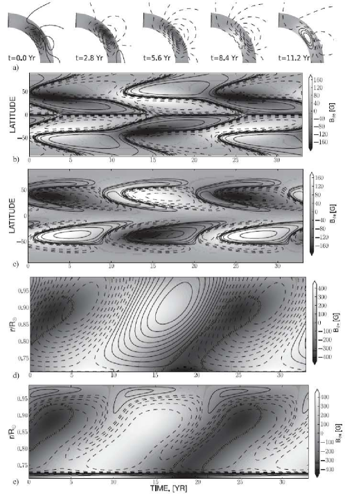
Figure 5: Illustration of dynamo model CQ3 : a) snapshots of the toroidal (gray scale) and poloidal (contours) magnetic field evolution for a half of the magnetic cycle; b) the time-latitude diagram for the toroidal magnetic field averaged over the depth range $0.95-0.99R_{\odot}$ (gray scale) and the poloidal field (contours, in range $\pm 3$ G); c) the time-latitude diagram for the toroidal magnetic field (gray scale) and the current helicity (contours, in range $\pm 2\ 10^{-4}$ G²m^-1); d) the time-radius diagram at latitude $30^{\circ}$ for the toroidal magnetic field (gray scale) and the poloidal field (contours, in range $\pm 3$ G); e) the time-radius diagram at latitude $30^{\circ}$ for the toroidal magnetic field (gray scale) and the current helicity (contours, in range $-2\ 10^{-4}\div 2\ 10^{-3}$ G²m^-1).

Model CQ3 is most relevant for comparison with observations. This case qualitatively reproduces the basic features of the solar cycle. Figure 5 shows snapshots of toroidal and poloidal fields, the time-latitude diagram of the near surface toroidal magnetic field, and the current helicity evolution, and the time-radius diagrams for the magnetic field and current helicity for this model. The time-laltitude diagrams illustrate the migration of the toroidal and poloidal fields and polarity reversal. The time-radius diagrams show migration of the magnetic field with radius at $30^{\circ}$ latitude, and an interesting concentration of the field at $r/R_{\odot}\sim 0.9-0.92$, or $60-70$Mm below the surface. This concentration is related to the second maximum of the dynamo wave when it propogates from the bottom of the convection zone to the surface.

Our results show that the current helicity changes the sign in the near surface layers at the begining of the cycle. A similar behaviour was found in observations of Zhang et al. (2010) (see their Fig.2). Our initial comparison of the current helicity pattern produced by the model reveals some disagreements with observations, e.g., the model does not show the change of the current helicity sign near the equator at the end of sunspot cycle. This problem needs a separate study, which should include a more sophisticated description of the helicity fluxes. The time-radius diagram at latitude $30^{\circ}$ for the toroidal magnetic field and the current helicity (Figure 5e) shows that that in the bulk of the convection zone the current helicity does not change much with time, and that the helicity is nearly constant near the bottom of the convection zone. In the north hemisphere the magnetic helicity is positive at the bottom of the convection zone because the kinetic part of the $\alpha$ effect is negative there (also see, Pipin & Kosovichev (2011) and Figure 1 there). In the near-surface layer the sign of the current helicity changes at the rising phase of the cycle.

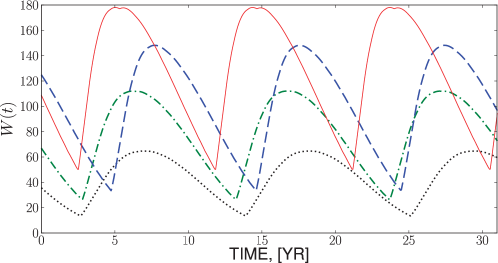
Figure 6: The asymmetry of sunspot number parameter W in the series of dynamo models WR2 (Table 1) calculated for various values of $C_{\alpha}$: $0.03$(dots), $0.04$ (dot-dashed curve), $0.05$ (dashed curve) and $0.06$ (solid curve).

Model CQ3 clearly shows asymmetry between the growth and decay phases of the sunspot number parameter $W(t)$. We find that the asymmetry increases with increase of the amplitude of the cycle, i.e., with increase of $\alpha$-effect parameter $C_{\alpha}$ (see Figure 6). It is expected that for the higher $C_{\alpha}$ the dynamo period is shorter (see, e.g., Parker, 1979) . This motivates us to look at the period - amplitude relationship for our model and also at the amplitude dependence on the growth/decay rate by computing a series of models WR1, WR2, WR3 for various values of $C_{\alpha}$ and $R_{\chi}$. The results for the asymmetry parameter as well as the cycle period are summarized in Table 1. We compare the model results with the asymmetry estimated from the monthly smoothed sunspot number provided by the SIDC. The data set was additionally smoothed by means of the Wiener filter. After this, we divided the whole data set covering the time period from 1749 to 2010, into separate sunspot cycles. The cycles were divided by a program that catches the sequences of the sunspot minima. For each cycle we estimate the growth rate by a ratio of the cycle amplitude to the growth time. Similarly, the decay rate was defined.

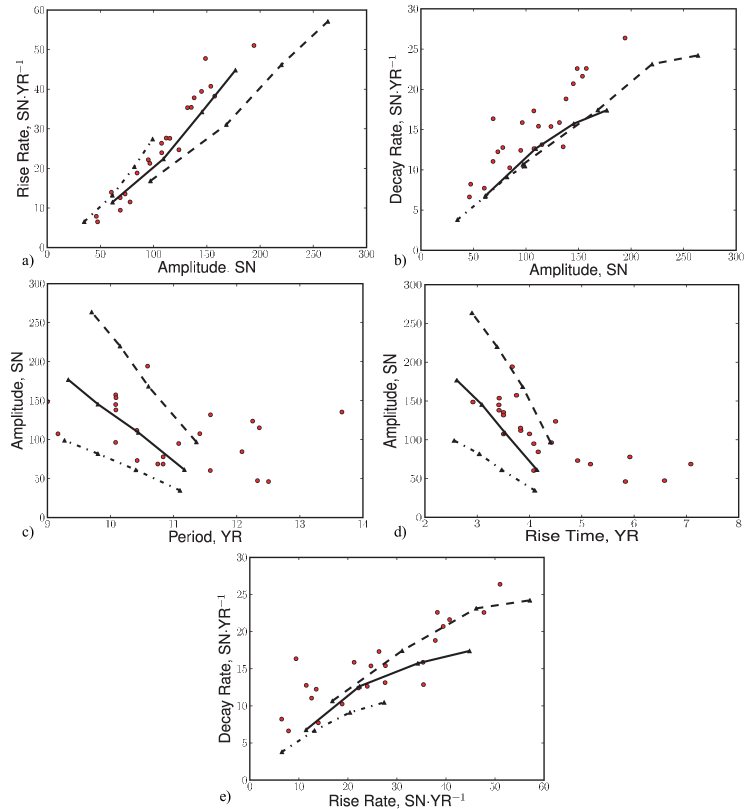
Figure 7: The Waldmeier’s (1935) relations in the models WR1 (dashed line), WR2 (solid line) and WR3 (dot-dashed line): a) amplitude - rise rate, b) amplitude - decay rate, c) period - amplitude, d) rise time - amplitude, e) rise - decay rates, g) rise - decay times. The results from the SIDC sunspot data are shown by circles.

Figure 7 compares the model with these estimates in the form of the Waldmeier’s (1935) relations: a) amplitude - rise rate, b) amplitude - decay rate, c) period - amplitude, d) rise time - amplitude, e) rise vs decay rates and g) rise vs decay times. The results obtained from the experimental data set confirm the findings of other authors (see, Vitinsky et al., 1986; Hathaway et al., 2002; Cameron & Schüssler, 2007; Kitiashvili & Kosovichev, 2009; Karak & Choudhuri, 2011). The computed dynamo models (WR1, WR2 and WR3) for a given range of the $\alpha$-effect parameter $C_{\alpha}=0.03-0.06$ and magnetic helicity dissipation rate $R_{\chi}=50-200$) correspond reasonably well to the data points. However, there are differences. One possible source of the difference between the model and the data is clarified in Figure 7(e), which shows correlation between the rise and decay rates in the solar cycles. We find that for most solar cycles the rise rate is higher than the decay rate. The mean asymmetry parameter is $\overline{A}_{W}\approx 0.68\pm 0.31$ . As seen in Figure 7, our models have smaller $A_{W}$ . Thus, our dynamo models produce more asymmetric $W$ profiles than the observed sunspot number. Increasing or decreasing the helicity dissipation by changing $R_{\chi}$ did not improve the agreement with the observations.

It is clear that more studies of the turbulent properties of the Sun are necessarily. Nevertheless, the initial results of the dynamo models shaped by the subsurface shear layer are encouraging.

4 Discussion and conclusion

The paper presents a study of a solar dynamo model operating in the bulk of the convection zone with the toroidal magnetic field flux shaped into the time-latitude “butterfly” diagram in the subsurface rotational shear layer. We explore how this type of dynamo may depend on the radial variations of turbulent parameters and the differential rotation near the surface. The mean-field dynamo model takes into account the evolution of the magnetic helicity and describes its nonlinear feedback on the generation of the large-scale magnetic field by the $\alpha$-effect. We compare the magnetic cycle characteristics predicted by the model, including the cycle asymmetry and the duration - amplitude relation (Waldmeier’s effects) with the observed sunspot cycle properties. We show that the model qualitatively reproduces the basic properties of the solar cycles. However, the model cycles are systematically more asymmetric than the observed cycles.

In section 3.1, it was shown that the radial profiles of the turbulent diffusivity and the density stratification scale in the sub-surface layer (between $0.95-0.99R_{\odot})$ may significantly influence the dynamo properties. In particular, the surface-shear shaped dynamo model favors the negative gradient of turbulent diffusivity in the sub-surface layer as follows from the standard solar model. This is contrary to the positive gradient of turbulent diffusivity often used in flux-transport dynamo models (e.g., Karak & Choudhuri, 2011). In our model, a steeper gradient of the magnetic diffusivity results in a stronger toroidal magnetic field, a higher latitudinal migration speed and a longer magnetic field decay time in the surface layer. We found that the downward turbulent pumping of the horizontal magnetic field (associated with either toroidal or meridional magnetic field components) brings the dynamo properties in better agreement with observations, increasing the period of the magnetic cycle for a given turbulent diffusivity profile. The model shows the asymmetry between the rise and decay rates (and duration phases) of the toroidal magnetic field. The asymmetry increases with the increase of the turbulent diffusivity gradient in the sub-surface layer.

The models shows a clear dependence of the asymmetry parameter (the ratio between the cycle’s decay and rise rates) on the magnetic cycle strength. We compared a sunspot number parameter previously suggested by Bracewell (1988) with statistical properties of the solar cycle. Our model qualitatively reproduces the known properties, such as the Waldmeier’s relations and the period - amplitude dependence. In particular, Figure 7e shows that the asymmetry is one of the basic features of the sunspot cycle activity (see also, Vitinsky et al., 1986).

In our model this asymmetry depends on the parameters of the turbulent diffusivity in the near surface layer and on the rate of the magnetic helicity dissipation. If the magnetic helicity dissipation rate is higher, the asymmetry is smaller. The magnetic helicity dissipation rate influences the amount of the total magnetic flux produced in the Sun. According to Schrijver & Harvey (1994) the total magnetic flux produced during a solar cycle is about $10^{24}$$\mathrm{{Mx}}$. The models presented in the paper satisfy this constraint. The estimated amount of magnetic helicity loss in the dynamo model is about $10^{45}$ $\mathrm{Mx}^{2}$ per cycle.

Thus, we conclude that the dynamo models with the subsurface shear layer can satisfy the global constraints on the total magnetic flux produced by the dynamo and are able to qualitatively reproduce the known statistical properties of the solar cycle, like the Waldmeier’s effects and the period - amplitude relation. We expect that the model can be further developed taking into account more accurately the turbulent properties of the sub-surface shear layer. The accurate description of the magnetic helicity dissipation is also important for the future progress. Direct numerical simulations of the convective turbulence and helioseismological data analysis techniques should help to improve our knowledge of the subsurface shear layer and the physics of solar dynamo.

5 Acknowledgements

This work was supported by NASA LWS NNX09AJ85G grant and partially by RFBR grant 10-02-00148-a.

6 Appendix

We describe some parts of the mean-electromotive force. The basic formulation is given in P08. For this paper we reformulate tensor $\alpha_{i,j}^{(H)}$, which represents the hydrodynamical part of the $\alpha$-effect, by using Eq.(23) from P08 in the following form,

$$\alpha_{ij}^{(H)} = \delta_{ij}\left\{3\eta_{T}\left(f_{10}^{(a)}\left(\mathbf{e}\cdot\boldsymbol{\Lambda}^{(\rho)}\right)+f_{11}^{(a)}\left(\mathbf{e}\cdot\boldsymbol{\Lambda}^{(u)}\right)\right)\right\}+$$

$$+ e_{i}e_{j}\left\{3\eta_{T}\left(f_{5}^{(a)}\left(\mathbf{e}\cdot\boldsymbol{\Lambda}^{(\rho)}\right)+f_{4}^{(a)}\left(\mathbf{e}\cdot\boldsymbol{\Lambda}^{(u)}\right)\right)\right\}$$

$$+ 3\eta_{T}\left\{\left(e_{i}\Lambda_{j}^{(\rho)}+e_{j}\Lambda_{i}^{(\rho)}\right)f_{6}^{(a)}+\left(e_{i}\Lambda_{j}^{(u)}+e_{j}\Lambda_{i}^{(u)}\right)f_{8}^{(a)}\right\}.$$

The contribution of magnetic helicity $\overline{\chi}=\overline{\mathbf{a\cdot}\mathbf{b}}$ ($\mathbf{a}$ is a fluctuating vector magnetic field potential) to the $\alpha$-effect is defined as $\alpha_{ij}^{(M)}=C_{ij}^{(\chi)}\overline{\chi}$, where

$$C_{ij}^{(\chi)}=2f_{2}^{(a)}\delta_{ij}\frac{\tau_{c}}{\mu_{0}\overline{\rho}\ell^{2}}-2f_{1}^{(a)}e_{i}e_{j}\frac{\tau_{c}}{\mu_{0}\overline{\rho}\ell^{2}}.$$ (5)

The turbulent pumping, $\gamma_{i,j}$, is also part of the mean electromotive force in Eq.(23)(P08). Here we rewrite it in a more traditional form (cf, e.g., Brandenburg & Subramanian, 2005; Rädler et al., 2003),

$$\gamma_{ij}=3\eta_{T}\left\{f_{3}^{(a)}\Lambda_{n}^{(\rho)}+f_{1}^{(a)}\left(\mathbf{e}\cdot\boldsymbol{\Lambda}^{(\rho)}\right)e_{n}\right\}\varepsilon_{inj}-3\eta_{T}f_{1}^{(a)}e_{j}\varepsilon_{inm}e_{n}\Lambda_{m}^{(\rho)},$$ (6)

The effect of turbulent diffusivity, which is anisotropic due to the Coriolis force, is given by:

$$\eta_{ijk}=3\eta_{T}\left\{\left(2f_{1}^{(a)}-f_{1}^{(d)}\right)\varepsilon_{ijk}-2f_{1}^{(a)}e_{i}e_{n}\varepsilon_{njk}\right\}.$$ (7)

Functions $f_{\{1-11\}}^{(a,d)}$ depend on the Coriolis number $\Omega^{*}=2\tau_{c}\Omega_{0}$ and the typical convective turnover time in the mixing-length approximation: $\tau_{c}=\ell/u^{\prime}$. They can be found in P08. The turbulent diffusivity is parametrized in the form, $\eta_{T}=C_{\eta}\eta_{T}^{(0)}$, where $\eta_{T}^{(0)}={\displaystyle\frac{u^{\prime}\ell}{3}}$ is the characteristic mixing-length turbulent diffusivity, $u^{\prime}$ is the RMS convective velocity, $\ell$ is the mixing length, $C_{\eta}$ is a constant to control the intensity of turbulent mixing. The others quantities in Eqs.(6,6,7) are: $\mathbf{\boldsymbol{\Lambda}}^{(\rho)}=\boldsymbol{\nabla}\log\overline{\rho}$ is the density stratification scale, $\mathbf{\boldsymbol{\Lambda}}^{(u)}=\boldsymbol{\nabla}\log\left(\eta_{T}^{(0)}\right)$ is the scale of turbulent diffusivity, $\mathbf{e}=\boldsymbol{\Omega}/\left|\Omega\right|$ is a unit vector along the axis of rotation. Equations (6,6,7) take into account the influence of the fluctuating small-scale magnetic fields, which can be present in the background turbulence and stem from the small-scale dynamo (see discussions in Frisch et al., 1975; Moffatt, 1978; Vainshtein & Kitchatinov, 1983; Kleeorin et al., 1996; Brandenburg & Subramanian, 2005). In our paper, the parameter $\varepsilon={\displaystyle\frac{\overline{\mathbf{b}^{2}}}{\mu_{0}\overline{\rho}\overline{\mathbf{u}^{2}}}}$, which measures the ratio between the magnetic and kinetic energies of fluctuations in the background turbulence, is assumed equal to 1. This corresponds to the energy equipartition. The quenching function of the hydrodynamical part of $\alpha$-effect is defined by

$$\psi_{\alpha}=\frac{5}{128\beta^{4}}\left(16\beta^{2}-3-3\left(4\beta^{2}-1\right)\frac{\arctan\left(2\beta\right)}{2\beta}\right).$$ (8)

Note, in notation of P08 $\psi_{\alpha}=-3/4\phi_{6}^{(a)}$, and $\beta={\displaystyle\frac{\left|\overline{B}\right|}{u^{\prime}\sqrt{\mu_{0}\overline{\rho}}}}$.

References

- Antia et al. (1998) Antia, H. M., Basu, S., & Chitre, S. M. 1998, MNRAS, 298, 543
- Benevolenskaya et al. (1999) Benevolenskaya, E. E., Hoeksema, J. T., Kosovichev, A. G., & Scherrer, P. H. 1999, ApJ, 517, L163
- Birch (2011) Birch, A. C. 2011, Journal of Physics Conference Series, 271, 012001
- Bracewell (1988) Bracewell, R. N. 1988, MNRAS, 230, 535
- Brandenburg (2005) Brandenburg, A. 2005, ApJ, 625, 539
- Brandenburg & Subramanian (2005) Brandenburg, A., & Subramanian, K. 2005, Phys. Rep., 417, 1
- Brandenburg & Subramanian (2005) Brandenburg, A., & Subramanian, K. 2005, Phys. Rep., 417, 1
- Brandenburg et al. (2007) Brandenburg, A., Käpylä, P. J., Mitra, D., Moss, D., & Tavakol, R. 2007, Astronomische Nachrichten, 328, 1118
- Cameron & Schüssler (2007) Cameron, R., & Schüssler, M. 2007, ApJ, 659, 801
- Choudhuri et al. (1995) Choudhuri, A. R., Schussler, M., & Dikpati, M. 1995, A&A, 303, L29+
- Drobyshevski & Yuferev (1974) Drobyshevski, E. M., & Yuferev, V. S. 1974, Journal of Fluid Mechanics, 65, 33
- Frisch et al. (1975) Frisch, U., Pouquet, A., Léorat, J., & A., M. 1975, J. Fluid Mech., 68, 769
- Guerrero et al. (2010) Guerrero, G., Chatterjee, P., & Brandenburg, A. 2010, MNRAS, 409, 1619
- Hathaway et al. (2002) Hathaway, D. H., Wilson, R. M., & Reichmann, E. J. 2002, Sol. Phys., 211, 357
- Karak & Choudhuri (2011) Karak, B. B., & Choudhuri, A. R. 2011, MNRAS, 410, 1503
- Kitchatinov (1991) Kichatinov, L. L. 1991, Astron. Astrophys., 243, 483
- Kitchatinov et al. (2000) Kitchatinov, L. L., Mazur, M. V., & Jardine, M. 2000, A&A, 359, 531
- Kitiashvili & Kosovichev (2009) Kitiashvili, I. N., & Kosovichev, A. G. 2009, Geophysical and Astrophysical Fluid Dynamics, 103, 53
- Kitiashvili & Kosovichev (2010) Kitiashvili, I. N., & Kosovichev, A. G. 2010, in IAU Symposium, Vol. 264, IAU Symposium, ed. A. G. Kosovichev, A. H. Andrei, & J.-P. Rozelot, 202–209
- Kleeorin et al. (1996) Kleeorin, N., Mond, M., & Rogachevskii, I. 1996, A&A, 307, 293
- Kleeorin et al. (2000) Kleeorin, N., Moss, D., Rogachevskii, I., & Sokoloff, D. 2000, A&A, 361, L5
- Kleeorin & Rogachevskii (1999) Kleeorin, N., & Rogachevskii, I. 1999, Phys. Rev.E, 59, 6724
- Kleeorin & Ruzmaikin (1982) Kleeorin, N. I., & Ruzmaikin, A. A. 1982, Magnetohydrodynamics, 18, 116
- Mitra et al. (2010) Mitra, D., Candelaresi, S., Chatterjee, P., Tavakol, R., & Brandenburg, A. 2010, Astronomische Nachrichten, 331, 130
- Mitra et al. (2011) Mitra, D., Moss, D., Tavakol, R., & Brandenburg, A. 2011, A&A, 526, A138
- Moffatt (1978) Moffatt, H. K. 1978, Magnetic Field Generation in Electrically Conducting Fluids (Cambridge, England: Cambridge University Press)
- Parker (1979) Parker, E. N. 1979, Cosmical magnetic fields: Their origin and their activity (Oxford: Clarendon Press)
- Parker (1993) Parker, E. N. 1993, ApJ, 408, 707
- Pipin (2008) Pipin, V. V. 2008, Geophysical and Astrophysical Fluid Dynamics, 102, 21
- Pipin & Kosovichev (2011) Pipin, V. V., & Kosovichev, A. G. 2011, ApJ, 727, L45
- Pipin & Kosovichev (2011) Pipin, V. V., & Kosovichev, A. G. 2011, ApJ(accepted)
- Rädler et al. (2003) Rädler, K.-H., Kleeorin, N., & Rogachevskii, I. 2003, Geophys. Astrophys. Fluid Dyn., 97, 249
- Ruediger & Brandenburg (1995) Ruediger, G., & Brandenburg, A. 1995, A&A, 296, 557
- Schrijver & Harvey (1994) Schrijver, C. J., & Harvey, K. L. 1994, Sol. Phys., 150, 1
- SIDC (2010) SIDC. 2010, Monthly Report on the International Sunspot Number, online catalogue, http://www.sidc.be/sunspot-data/
- Stix (2002) Stix, M. 2002, The Sun. An Introduction (Springer)
- Tobias & Weiss (2007) Tobias, S., & Weiss, N. 2007, in The Solar Tachocline, ed. D. W. Hughes, R. Rosner, & N. O. Weiss, 319
- Vainshtein & Cattaneo (1992) Vainshtein, S. I., & Cattaneo, F. 1992, ApJ, 393, 165
- Vainshtein & Kitchatinov (1983) Vainshtein, S. I., & Kitchatinov, L. L. 1983, Geophys. Astrophys. Fluid Dynam., 24, 273
- Vishniac & Cho (2001) Vishniac, E. T., & Cho, J. 2001, Astrophys. J., 550, 752
- Vitinsky et al. (1986) Vitinsky, Y. I., Kopecky, M., & Kuklin, G. V. 1986, The statistics of sunspots (Statistika pjatnoobrazovatelnoj dejatelnosti solntsa) (Nauka, Moscow), 298pp
- Yoshimura (1975) Yoshimura, H. 1975, ApJ, 201, 740
- Zhang et al. (2010) Zhang, H., Sakurai, T., Pevtsov, A., Gao, Y., Xu, H., Sokoloff, D. D., & Kuzanyan, K. 2010, MNRAS, 402, L30