Bayesian Inference Analysis of Unmodelled Gravitational-Wave Transients

Abstract

We report the results of an in-depth analysis of the parameter estimation capabilities of BayesWave, an algorithm for the reconstruction of gravitational-wave signals without reference to a specific signal model. Using binary black hole signals, we compare BayesWave’s performance to the theoretical best achievable performance in three key areas: sky localisation accuracy, signal/noise discrimination, and waveform reconstruction accuracy. BayesWave is most effective for signals that have very compact time-frequency representations. For binaries, where the signal time-frequency volume decreases with mass, we find that BayesWave’s performance reaches or approaches theoretical optimal limits for system masses above approximately 50 $M_{\odot}$. For such systems BayesWave is able to localise the source on the sky as well as templated Bayesian analyses that rely on a precise signal model, and it is better than timing-only triangulation in all cases. We also show that the discrimination of signals against glitches and noise closely follow analytical predictions, and that only a small fraction of signals are discarded as glitches at a false alarm rate of 1/100 y. Finally, the match between BayesWave-reconstructed signals and injected signals is broadly consistent with first-principles estimates of the maximum possible accuracy, peaking at about $0.95$ for high mass systems and decreasing for lower-mass systems. These results demonstrate the potential of unmodelled signal reconstruction techniques for gravitational-wave astronomy.

1 Introduction

The recent direct detection of gravitational waves by Advanced LIGO and Advanced Virgo has opened a new window in observational astronomy. On 14 September 2015, LIGO made the first ever observation of a binary black hole (BBH) merger [1]. The signal, denoted GW150914, has been followed by other detections of BBH mergers — GW151226 [2], GW170104 [3], GW170608 [4], and GW170814 [5] — and by the detection of a binary neutron star inspiral, GW170817 [6]. The BBH observations have revealed the existence of a previously unknown population of high-mass ($>20\,M_{\odot}$) black holes, with implications for our understanding of stellar evolution [7, 8, 9, 10], and have allowed the first tests of general relativity in the dynamical, strong-field regime [11, 2, 3].

The interpretation of these signals has relied upon precise signal models (“templates”) [12] that can be compared to the data. However, there are many possible emission mechanisms beyond BBHs for which the gravitational wave (GW) radiation cannot be easily modelled, such as core-collapse supernovæ [13, 14, 15, 16, 17], post-merger emission by hypermassive neutron stars in binary neutron star mergers [18, 19, 20, 21, 22, 23, 24, 25], and magnetar flares [26, 27, 28], for which matched filtering is not applicable. This has spurred the development of tools for the detection and characterisation of generic GW transients (a.k.a., “bursts”) [29, 30, 31, 32, 33, 34]. Among them is BayesWave [35], a Bayesian parameter estimation algorithm for the reconstruction of generic GW transients. Instead of relying on a precise signal model, BayesWave fits linear combinations of basis functions to the data in a manner consistent with either a GW or background noise artifacts (“glitches”). Given a potential GW trigger, BayesWave performs a Bayesian analysis under the signal and the glitch hypotheses, reconstructs the gravitational waveform, and provides estimates of model-independent parameters, such as the signal duration, bandwidth, and sky location. This tool was used successfully, for example, in the follow-up of GW150914 and GW170104 [1, 36, 3].

In this paper, we subject BayesWave to a series of tests in order to validate it and assess its performance against first-principles estimates. While there have been some studies of the performance of such algorithms for various kinds of burst signals (see for example [37, 38, 39, 40]), very little has been done to compare their performance to first-principles expectations; i.e., we do not know if presently available tools are performing close to optimally, or if there is significant room for improvement. We address this by assessing BayesWave in three critical areas:

1. Sky localisation: How accurately can BayesWave determine the direction to the GW source, compared to ideal matched-filtering algorithms?

2. Signal–glitch discrimination: How robustly can BayesWave distinguish true GW signals from non-Gaussian background noise artifacts?

3. Waveform reconstruction: How does the accuracy of BayesWave’s reconstructed gravitational waveforms compare to first principles estimates of the possible accuracy of unmodelled reconstructions?

We answer these questions by applying BayesWave to a set of simulated BBH signals added to simulated Advanced LIGO and Advanced Virgo data [41]. While accurate templates are available for BBH signals, BayesWave does not use this information. Using BBH templated signals for our tests allows us to compare the performance of BayesWave to the case of ideal matched-filtering, which does rely on a precise signal model. Despite not using a signal model, we find that the performance of BayesWave is remarkably close to optimal in most cases, and we note the conditions under which performance is less than optimal.

The paper is organised as follows. In Sec. 2, we briefly discuss the BayesWave algorithm. In Sec. 3 we describe the test performed to assess the performance of BayesWave and discuss our results. Finally, our conclusions are summarized in Sec. 4.

2 BayesWave

BayesWave is a Bayesian follow-up pipeline for GW triggers. It is designed to distinguish GW signals from non-stationary, non-Gaussian noise transients (i.e., glitches) in interferometric GW detector data, and to characterize the signals themselves [35, 42]. BayesWave uses a multi-component, parametric noise model of variable dimension that accounts for instrument glitches. These are modeled using a linear combination of Morlet-Gabor continuous wavelets. A trans-dimensional reversible jump Markov chain Monte Carlo algorithm allows for the number of wavelets to vary and to explore the parameters of each wavelet. GW transients of astrophysical origin are (independently) modelled with the same technique: a single GW signal model is built at the center of the Earth and projected onto each detector in the network, taking into account the response of the instrument and the source sky-location, which feeds two parameters (i.e., right ascension and declination) into the reconstruction effort. A linear combination of wavelets constituting a glitch model is instead built for each individual detector. In other words, there is a requirement for signals to appear coherently in the data, but not for glitches.

The BayesWave algorithm compares the following hypotheses: (1) the data contain only Gaussian noise, (2) the data contain Gaussian noise and glitches, and (3) the data contain Gaussian noise and a GW signal. The comparison is performed in terms of the marginalized posterior (evidence) for each hypothesis. When testing the signal hypothesis, BayesWave provides a waveform reconstruction, and posterior distributions for the source sky location parameters and signal characteristics, such as duration, bandwidth, energy, central frequency. These may be used to compare the data to theoretical models and to assess the performance of the pipeline.

BayesWave has been used in a number of studies so far. Notably, it was used as a follow-up analysis to candidate and background events found by the coherent WaveBurst (cWB) pipeline [29, 30] and matched-filter searches during the first two Advanced LIGO observing runs [36, 43, 44]. BayesWave localized the source of the GW150914 event in a $101$ square degree region with 50% confidence and set a false alarm rate (FAR) of $1$ in $67400$ years. Further, [36] tested the ability of BayesWave in recovering simulated BBH signals for sources similar to GW150914. The match between the reconstructed and injected waveforms was found to be vary between 90% and 95% for systems with total mass between $\sim 60$ $\mathrm{M}_{\odot}$ and $\sim 100$ $\mathrm{M}_{\odot}$, and an injected network signal-to-noise ratio (SNR) of $20$. The sensitivity range, which is tightly correlated to the total mass and the effective spin of the system, was found to be in the $400$–$800$ Mpc interval. In general, the combined cWB-BayesWave data analysis pipeline was shown to allow for detections across a range of waveform morphologies [45, 46], with confidence increasing with the waveform complexity (at a fixed SNR). This is the case because glitches can be confused more easily with simple, short GW transients, rather than with complex waveforms in coherent data. Finally, a recent study [40] shows that the two-detector Advanced LIGO network will be able to achieve an $85$% and $95$% match for GW signals with network SNR below $\sim 20$ and $\sim 50$, respectively. In the same study, the median searched area and the median angular offset for BBH sources with total mass between $30\,M_{\odot}$ and $50\,M_{\odot}$ were found to be $99.2$ square degrees and $25.1$ degrees, respectively.

3 Procedure and Results

3.1 Simulated Signal Population

The source population we choose for our study consists of non-spinning merging BBHs. The values of the individual BH masses that we select are $5\,M_{\odot}$, $10\,M_{\odot}$, $50\,M_{\odot}$, and $100\,M_{\odot}$. We consider all 10 possible mass combinations: $(5,5)\,M_{\odot}$, $(5,10)\,M_{\odot}$, $(5,50)\,M_{\odot}$, $(5,100)\,M_{\odot}$, $(10,10)\,M_{\odot}$, $(10,50)\,M_{\odot}$, $(10,100)\,M_{\odot}$, $(50,50)\,M_{\odot}$, $(50,100)\,M_{\odot}$, and $(100,100)\,M_{\odot}$. This population is convenient for a number of reasons.

1. The majority of GW signals detected by LIGO to date were emitted by BBH sources [1, 2, 3, 4, 5], and BBH mergers are expected to dominate the population of GWs that we detect with second-generation instruments [47]. The BH masses of the sources detected so far (both the binary constituents and the merger remnants) are all encompassed by our choice of parameter space.

2. Accurate and computationally tractable waveform models exist for these signals, allowing us to compare the BayesWave performance to that of optimal (template-based) algorithms as reported in the literature. Specifically, we use the so-called IMRPhenomB approximant [48].

3. BayesWave may be able to resolve aspects of the waveform that are not included in current templated analyses, such as precessing spins or eccentricity. Ultimately it will be useful to characterise BayesWave for the entire family of BBH signals: in this sense, our non-spinning study is a first step in this direction.

4. The SNR of signals from high-mass systems is concentrated in a small time-frequency volume, while the SNR of signals from low-mass systems, e.g., binary neutron stars [6], is spread over a much larger time-frequency volume. This allows us to probe the performance of BayesWave relative to templated algorithms as a function of the signal time-frequency volume, which along with the SNR is the key characteristic of a signal for burst detection algorithms [49].

For each of the 10 mass pairs we generate 20 signals, for a total of 200 simulations, with random sky position, inclination, and polarisation angle. The distances are selected randomly such that the coherent network SNR is in the range 10–35; i.e., we use realistic amplitudes for detectable signals. The signals are added to simulated data for the LIGO-Virgo network H1-L1-V1, which consists of Gaussian noise following the power spectral density model of [41]. As the BHs inspiral, the frequency of the GW signal increases until the two bodies merge and the GW emission cuts off. The merger frequency scales inversely with system mass, so signals from low-mass systems span the full LIGO/Virgo sensitive band and therefore have large effective bandwidth and time-frequency volume. For high-mass systems the effective bandwidth is much smaller and the signal is concentrated in a relatively small time-frequency volume. These will have implications for localisation accuracy and waveform reconstruction that are discussed later in the text.

For each simulation we analyse 4 s of data centred on the binary coalescence time, generated at a sampling rate of 1024 Hz. This data is fed into BayesWave for analysis. BayesWave reports the log evidence for signal vs. glitch and for signal vs. noise hypotheses, a sky map, reconstructed time-domain waveforms, spectrograms, and estimates of other properties such as duration, bandwidth, and the SNR recovered in each detector. In the following subsections we focus on BayesWave’s performance on spectrograms, signal vs. glitch discrimination, and the accuracy of sky localisation and waveform reconstruction.

3.2 Time-Frequency Signal Content

As shown in [46], the number of wavelets used by BayesWave to reconstruct a GW signal increases approximately linearly with SNR, at a rate that depends on the signal morphology (higher for more complex waveforms). This is consistent with the behaviour seen in our simulations. For the SNRs considered in our study, the average reconstructed SNR per wavelet is typically 5–10.

For inspiralling BBHs, the frequency increases until the two bodies merge and the gravitational-wave emission cuts off, as the remnant BH rings down. The merger frequency scales inversely with system mass: low-mass systems produce GW signals that have larger effective bandwidth and time-frequency volume than high-mass systems. Furthermore, the rate of frequency increase in the signal (“chirping”) increases with the system mass, so that high-mass systems have a much shorter duration in the detector sensitive band. Together these have an important consequence for burst algorithms such as BayesWave that rely on time-frequency decompositions: signals from low-mass systems are spread over a larger time-frequency area than signals from high-mass systems. Figure 1 shows example spectrograms of the simulated and recovered signals for the lowest- and highest-mass systems tested. The low-mass, $(5,5)\,M_{\odot}$, simulated signal shown on the top left panel occupies a time-frequency area greater than the high-mass, $(100,100)\,M_{\odot}$, simulated signal shown in the bottom left panel. As a result, BayesWave is able to recover all of the SNR of the high-mass signal (bottom right panel), but not all of the SNR of the low-mass signal (top right panel). Figure 2 confirms that the SNR is spread across a larger number of pixels as the system mass decreases. Generally, diluting a given total SNR among a larger number of pixels makes it more difficult for BayesWave to reconstruct the low-SNR portions of the signal. This typically results in a lower reconstructed SNR, duration, and bandwidth, which in turn lowers the accuracy of the sky localisation, signal classification and waveform reconstruction.

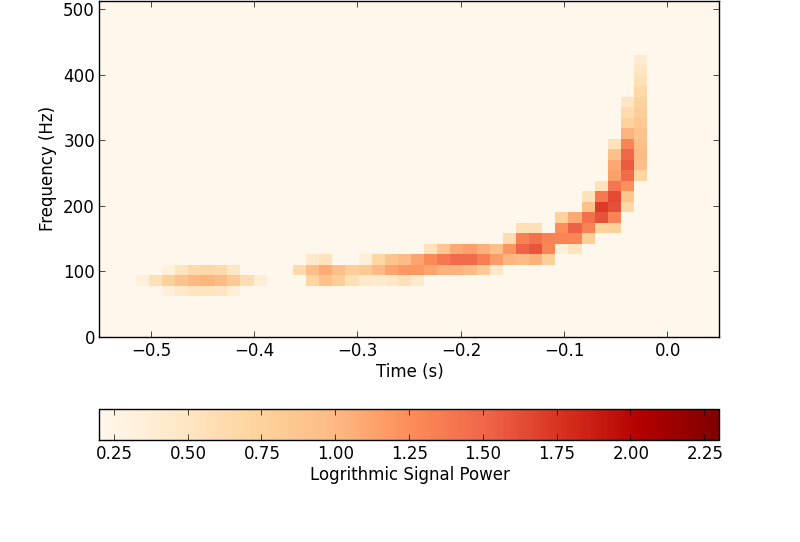
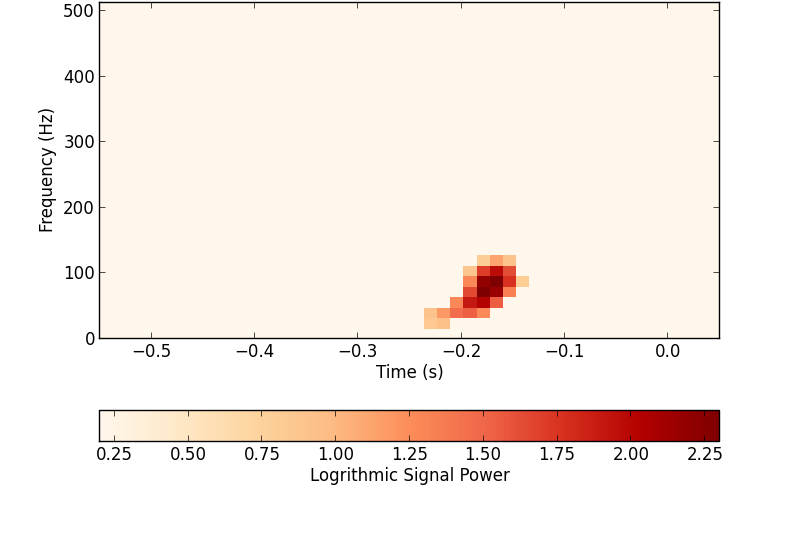
Figure 1: Whitened spectrograms for simulated and recovered signals. Top: (5,5) $M_{\odot}$ simulated (left) and recovered (right) signal. The SNR per time-frequency pixel is lowest at early times and low frequencies; BayesWave only recovers fragments of this portion of the signal. Bottom: (100,100) $M_{\odot}$ simulated (left) and recovered (right) signal. The SNR is concentrated into a small number of time-frequency pixels which are easily recovered by BayesWave.

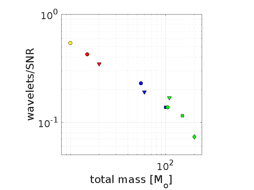
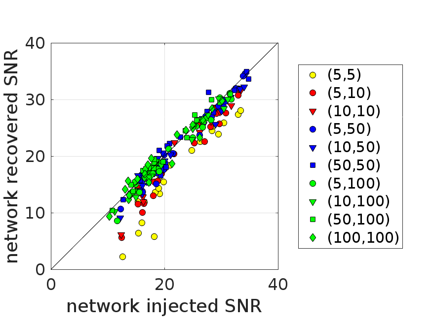
Figure 2: Left: Mean number of wavelets per unit injected network SNR vs. system total mass. As the system mass increases, the signal SNR in concentrated into a smaller time-frequency volume, and can be reconstructed with fewer wavelets. Right: Recovered network SNR vs. injected network SNR. BayesWave is able to recover the full SNR of high-mass systems, which occupy a small time-frequency volume. It systematically underestimates the SNR of low-mass systems, which occupy a larger time-frequency volume at a given SNR.

3.3 Sky Localisation

There are numerous empirical studies of the sky localisation capabilities of existing GW transient detection algorithms, particularly in the context of second-generation GW detector networks (see e.g. [37, 38, 39, 40]). The theoretical basis for sky localisation accuracy is best established for matched-filter searches for binary coalescences. As shown by Fairhurst [50, 51, 52, 53], the localisation is based primarily on triangulation via the time-of-arrival differences between the detector sites. The one-sigma measurement uncertainty in the time of arrival is given by

$$\sigma=\frac{1}{2\pi\rho\,\sigma_{f}}\,,$$ (1)

where $\rho$ is the matched-filter SNR in the detector and $\sigma_{f}$ is the effective bandwidth of the signal; see [51] for definitions. Ignoring the phase and amplitude measured in each detector, Fairhurst shows that one can construct a localisation matrix that defines the contours of fixed probability,

$$\mathbf{M}=\frac{1}{\sum_{k}\sigma_{k}^{-2}}\sum_{i,j}\frac{(\mathbf{d}_{i}-\mathbf{d}_{j})(\mathbf{d}_{i}-\mathbf{d}_{j})^{T}}{2\sigma_{i}^{2}\sigma_{j}^{2}}\,,$$ (2)

where $\mathbf{d}_{i}$ is the position vector of detector $i$ and $\sigma_{i}$ is the timing uncertainty in that detector. The expected sky localisation accuracy with containment probability $p$ is given by

$$A(p,\mathbf{r})=2\pi\sigma_{1}\sigma_{2}[-\log(1-p)]\,,$$ (3)

where $\sigma_{1},\sigma_{2}$ are the inverse square roots of the eigenvalues of the matrix $\mathbf{M}$ after it has been projected onto the sky in the direction $\mathbf{r}$,

$$\mathbf{M}(\mathbf{r})=\mathbf{P}(\mathbf{r})\,\mathbf{M}\,\mathbf{P}(\mathbf{r})\,,\quad\mathbf{P}(\mathbf{r})=\mathbf{I}-\mathbf{r}\mathbf{r}^{T}\,,$$ (4)

where $\mathbf{I}$ is the identity matrix. Since the approximation (3) ignores the phase and amplitude information, it can be considered as a worse-case estimate of the localisation capability.

As shown in [54] and [53], requiring a consistent signal phase and polarisation between the detectors improves the localisation accuracy by an amount which can be approximated by using a timing uncertainty of

$$\sigma_{t}^{c}=\frac{1}{2\pi\rho\,\sigma_{f}}\left(\frac{\sigma_{f}^{2}}{\bar{f^{2}}}\right)^{1/4}\,,$$ (5)

where $\overline{f^{2}}$ is the second frequency moment of the signal. Since $\overline{f^{2}}>\sigma_{f}^{2}$, Eq. (5) will yield smaller localisation areas. In their study of binary inspiral signals of total mass up to 20 $M_{\odot}$, Grover et al. demonstrated that this phase and polarisation correction reduces the predicted localisation areas by a factor of 2–3 relative to timing alone. Finally, Grover et al. also demonstrated that a full Bayesian analysis using signal templates achieves sky localisation accuracies that are still better by a median factor of 1.6; we take this Bayesian analysis to represent the “best possible” performance in the case where the signal waveform is known. [55] found a similar result for binary neutron star sources, with a median factor of $\sim 1.3$ for the 50% localisation area.

Table 1 and Figs. 3 and 4 compare the 50% and 90% localisation areas reported by BayesWave to the predictions of timing-only and phase-corrected triangulation. We see that BayesWave easily outperforms the timing-only predictions. It also outperforms the predictions of phase- and polarisation-corrected triangulation for all but the lowest-mass systems, despite not using a signal template. Indeed, for system masses above 50 M_⊙ the BayesWave performance is approximately equal to that of the optimal templated Bayesian analysis reported in Grover et al. [54].

We conclude that BayesWave is able to localise a gravitational-wave source on the sky as well as a templated analysis despite not using signal templates, provided the signal SNR is concentrated in a sufficiently small time-frequency volume ($\lesssim 10$ wavelets). Furthermore BayesWave still performs reasonably well — within a factor of 2 in area — for higher time-frequency volume signals even for large containment regions.

Table 1: Median ratio of 50% and 90% sky localisation areas reported by BayesWave to those predicted by triangulation. BayesWave typically outperforms the predictions of incoherent (timing-only) triangulation in almost all cases, and outperforms the predictions of coherent (phase- and polarisation-corrected) triangulation for systems of total mass above 50 M_⊙. For comparison, [54] report that the 50% localisations from an optimal templated Bayesian analysis are typically $\sim$0.6-0.7 of those of coherent triangulation [see also [55]]; we see that BayesWave performs comparably for system masses around 100 M_⊙ or more.

		Median BayesWave/triangulation ratio
$m_{1}$ $[M_{\odot}]$	$m_{2}$ $[M_{\odot}]$	50% area		90% area
		incoherent	coherent	incoherent	coherent
5	5	0.67	1.20	0.88	1.60
5	10	0.62	1.12	1.06	2.06
10	10	0.54	1.05	0.74	1.32
5	50	0.42	0.88	0.46	0.97
10	50	0.38	0.76	0.36	0.75
50	50	0.32	0.78	0.32	0.84
5	100	0.21	0.62	0.25	0.71
10	100	0.25	0.70	0.28	0.73
50	100	0.19	0.61	0.23	0.71
100	100	0.13	0.47	0.19	0.75

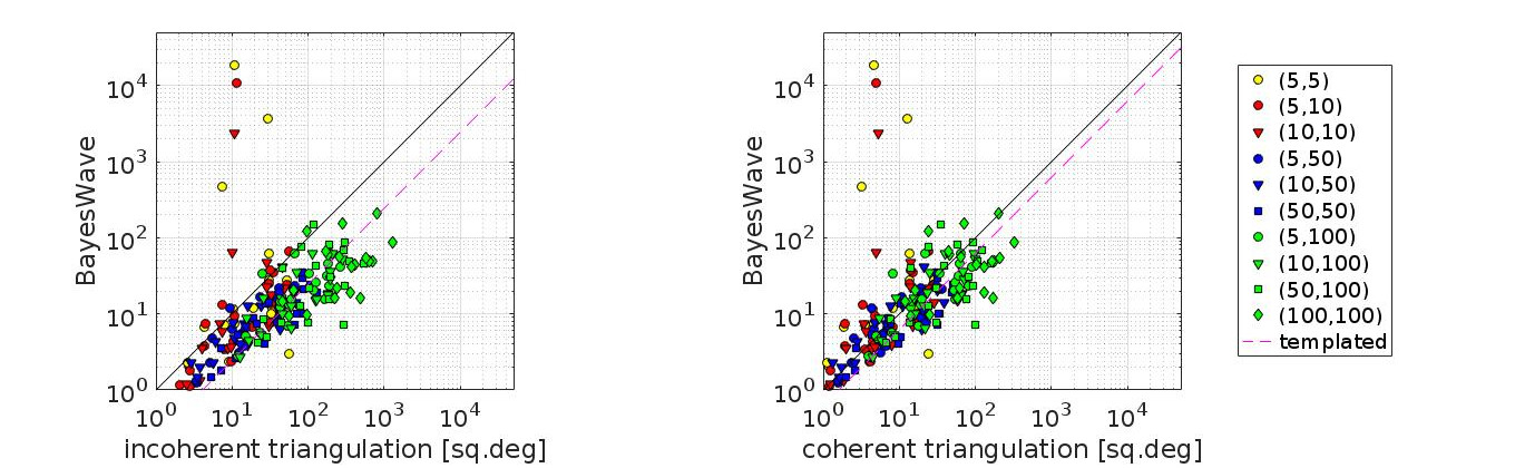
Figure 3: 50% containment localisation areas measured by BayesWave versus those predicted by timing-only “incoherent” triangulation (left) and phase- and polarisation-corrected “coherent” triangulation (right). The dashed line indicates the approximate median performance of a templated Bayesian analysis as reported in [54]. BayesWave systematically outperforms the timing-only predictions for all mass pairs. It also systematically outperforms the predictions of phase- and polarisation-corrected triangulation for all but the lowest-mass systems, despite not using a signal template. For system masses above 50 M_⊙ the BayesWave performance is approximately equal to that of the templated Bayesian analysis. In both cases smaller-bandwidth signals tend to have larger localisation areas, as expected. The small number of outliers are signals from low-mass systems that BayesWave was unable to reconstruct accurately.

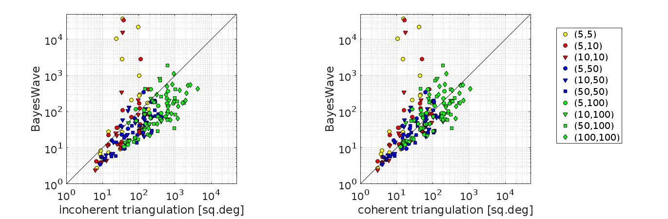
Figure 4: 90% containment localisation areas measured by BayesWave versus those predicted by timing-only “incoherent” triangulation (left) and phase- and polarisation-corrected “coherent” triangulation (right). BayesWave systematically outperforms the timing-only predictions for all mass pairs. It also systematically outperforms the predictions of phase- and polarisation-corrected triangulation for all but the lowest-mass systems, despite not using a signal template. In both cases smaller-bandwidth signals tend to have larger localisation areas, as expected. The small number of outliers are signals from low-mass systems that BayesWave was unable to reconstruct accurately.

3.4 Signal Classification

The confident detection of unmodelled transients depends on the ability to distinguish robustly true signals from the transient noise fluctuations (“glitches”) that are common features of the detector noise backgrounds [56]. Searches for generic GW transients typically rely on comparisons of weighted measures of the cross-correlation between detectors to the total energy in the data for signal-glitch discrimination (see, e.g., [57, 33, 30, 36]). BayesWave does this by calculating the log Bayes factors for the signal and glitch hypotheses. Under each hypothesis, the transient (either the result of the two GW polarizations, or the glitch time-series in each detector) is fit by a linear combination of Morlet-Gabor wavelets. The Bayes factor depends on both the quality of the fit and the priors; generally, signals which have high SNR-per-pixel throughout a large time-frequency volume are most easily distinguished from glitches. Littenberg et al. [46] argue that the signal-vs.-glitch log Bayes factor $\log\mathcal{B}_{\mathcal{S},\mathcal{G}}$ can be approximated by

$$\log\mathcal{B}_{\mathcal{S},\mathcal{G}} \simeq \frac{5N}{2}+5N\log\left(\frac{\rho}{\sqrt{N}}\right)$$ (6)

$$- \sum_{n=1}^{N}\log\left(2^{13/6}\pi^{2/3}\mathcal{Q}_{n}\right)$$

$$+ N\log V_{\lambda}+\left(2+\log\frac{\sqrt{\det\mathcal{C}_{Q}}}{4\pi^{2}}\right)$$

$$\approx \frac{5N}{2}+5N\log\left(\frac{\rho}{\sqrt{N}}\right)\,,$$

where $N$ is the number of wavelets, $\rho$ is the matched-filter SNR, $V_{\lambda}$ is the volume of the intrinsic parameter space, $\mathcal{C}_{Q}$ is the signal parameter covariance matrix, and $\mathcal{Q}_{n}$ is the quality factor of the $n^{\mathrm{th}}$ wavelet. Equation (6) is our approximation, made by keeping only the leading order terms.

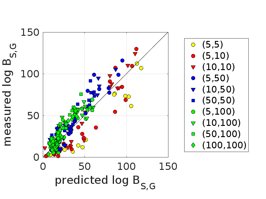
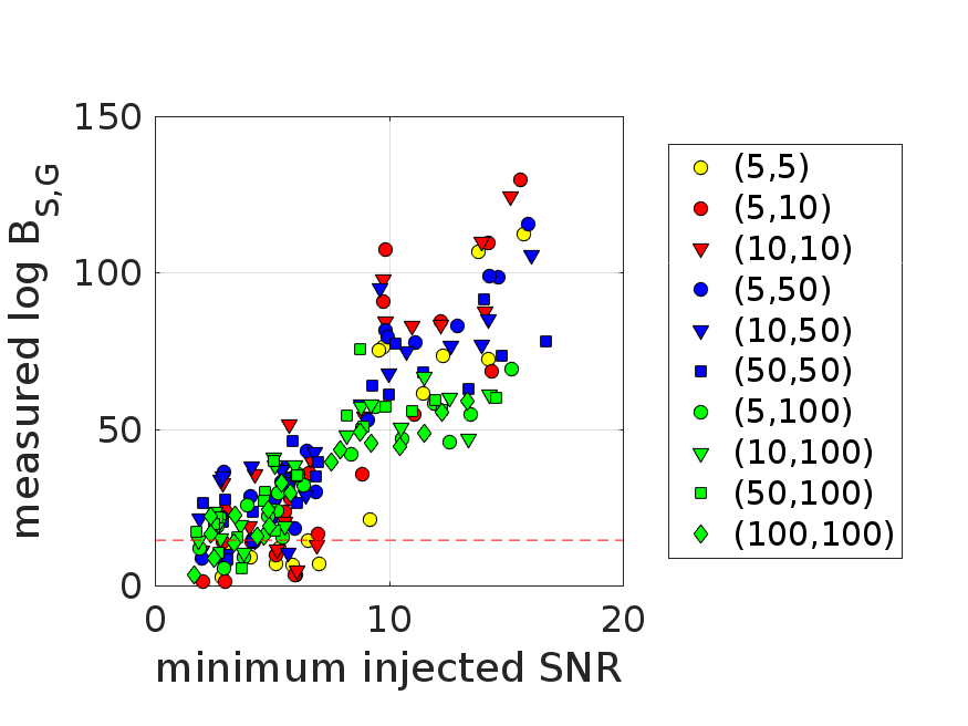
Figure 5: (left) Predicted and measured log Bayes factors for the Signal vs. Glitch test. The measured log Bayes factors are in good agreement with the predicted analytical expressions from [46] and [35], except for the lowest-mass systems, for which BayesWave is unable to recover the full SNR. (Right) Measured log Bayes factors vs. minimum injected SNR. The red dashed line indicates a $\log\mathcal{B}_{\mathcal{S},\mathcal{G}}$ threshold that corresponds to a FAR of 1/100 yr. Low time-frequency volume signals are distinguishable from glitches at this FAR provided the SNR is greater than 5–6 in all three detectors. High time-frequency volume signals are distinguishable for SNRs greater than 7–8 in all three detectors.

We compare the analytical approximation of $\mathcal{B}_{\mathcal{S},\mathcal{G}}$ in Eq. (6) with the measured BayesWave output for a range of BBH masses. As discussed in [46], signal-glitch discrimination improves with the number of detectors that see the transient. We find that the best predictions for $\mathcal{B}_{\mathcal{S},\mathcal{G}}$ come from using the minimum injected SNR for $\rho$ in Eq. (6); i.e., the lowest of the SNRs in H1, L1 or V1. The results are shown in the left panel of Fig. 5, where the correlation between measured and predicted $\log\mathcal{B}_{\mathcal{S},\mathcal{G}}$ is evident. The measured log Bayes factors are lower than predicted for the lowest-mass systems, because BayesWave is unable to recover the full SNR of these signals. Low-mass systems require higher SNR per time-frequency pixel, which in turn limits their reconstruction compared to high-mass systems. The predictive power of Eq. (6) can be improved further by using the minimum recovered SNR instead of the minimum injected SNR.

We can compare these results to the typical log Bayes factor for background noise to establish what real astrophysical signals could be recovered with high confidence. Using real LIGO noise from the 2009-10 run, Littenberg et al. [46] computed log Bayes factors for coincident events found by the cWB pipeline [29, 30] and showed that a threshold of $\log\mathcal{B}_{\mathcal{S},\mathcal{G}}=14.4$ corresponds to a FAR of 1/100 yr. In the first Advanced LIGO run, around the time of GW150914, the same FAR value corresponds to $\log\mathcal{B}_{\mathcal{S},\mathcal{G}}\sim 2$–$3$ (see Fig. 4 in [36]). For illustration, we use the higher of these ($14.4$) as an indicative threshold; this is represented by the red dashed line in the right panel of Fig. 5. We see that low time-frequency volume signals are distinguishable from glitches at this FAR provided the SNR is greater than 5–6 in all three detectors, while high time-frequency volume signals are distinguishable for SNRs greater than 7–8 in all three detectors.

Finally, we note that BayesWave also provides a log Bayes factor for the signal vs. Gaussian noise hypotheses. Cornish and Littenberg [35] show that this log Bayes factor can be approximated by

$$\log\mathcal{B}_{\mathcal{S},\mathcal{N}} = M^{2}\frac{\rho_{\mathrm{net}}^{2}}{2}+\Delta\ln\mathcal{O}$$ (7)

$$\approx M^{2}\frac{\rho_{\mathrm{net}}^{2}}{2}\,,$$

where $M$ is the match (discussed below) and $\rho_{\mathrm{net}}$ is the coherent network SNR. $\mathcal{O}$ is the Occam factor, which we ignore for our comparisons.

Figure 6 shows that the predicted $\log\mathcal{B}_{\mathcal{S},\mathcal{N}}$’s closely follow the measured $\log\mathcal{B}_{\mathcal{S},\mathcal{N}}$’s. As for $\log\mathcal{B}_{\mathcal{S},\mathcal{G}}$, we see that the measured log Bayes factors are (slightly) lower than the predicted ones for the lowest-mass systems, because BayesWave is unable to recover the full SNR of these signals.

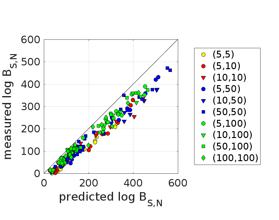
Figure 6: Predicted and measured log Bayes factors for the Signal vs. Gaussian noise test. The measured log Bayes factors are in very good agreement with predicted analytical expressions from [46] and [35] based on the total injected network SNR and the time-frequency volume of the signal. The measured log Bayes factors are systematically lower than the predicted ones for the lightest-mass (highest time-frequency volume) systems, for which BayesWave is unable to recover the full SNR.

3.5 Waveform Reconstruction

Many potential sources of GW transients, such as core-collapse supernovæ and hypermassive neutron stars formed in binary neutron star mergers, are too complicated to model accurately. In some cases even parts of the underlying physics are unknown (e.g., the neutron star equation of state). The ability to reconstruct the received $h(t)$ signal without reliance on accurate “templates” will therefore be crucial for the exploitation of GWs to probe new and unexpected systems.

First-principles estimation of the match between the true GW signal with SNR $\rho_{\mathrm{inj}}$ and a maximum-likelihood reconstruction of the signal based on a time-frequency pixel analysis can be estimated using only the recovered SNR $\rho_{\mathrm{rec}}$ and number of pixels $N$ [60],

$$M\simeq\frac{\rho_{\mathrm{rec}}}{\rho_{\mathrm{inj}}}\left(1+\frac{2N}{\rho_{\mathrm{rec}}^{2}}\right)^{-1/2}$$ (8)

with a one-sigma fractional uncertainty of

$$\frac{\delta M}{M}\simeq\frac{\sqrt{3}}{\rho_{\mathrm{rec}}}\,.$$ (9)

The $\rho_{\mathrm{rec}}/\rho_{\mathrm{inj}}$ factor in Eq. (8) is due to portions of the signal that are not included in the reconstruction, such as the low-frequency early-time portions of the low-mass signals. The factor in parentheses is due to the noise contamination of those pixels that are included in the reconstructed waveform. These expressions should be most accurate in the limit of high SNR per pixel, $\rho_{\mathrm{rec}}^{2}/N\gg 1$.

Figure 7 compares the mismatch, $1-M$, of the waveform reconstructed by BayesWave to the first-principles estimate from Eq. (8). We see that there is broad agreement between the two, with the measured mismatches typically about 50% higher than the first-principles estimate of the lowest achievable mismatch. Not surprisingly, the lowest mismatches are achieved for the signal with smallest time-frequency volume (high masses), where the entire signal in the sensitive band of the detectors is reconstructed. The highest mismatches are for the largest time-frequency volume signals (low masses), where BayesWave is unable to reconstruct the full signal. In these cases, the mismatch is dominated by the BayesWave reconstruction not including the full signal, as opposed to noise contamination of the reconstruction.

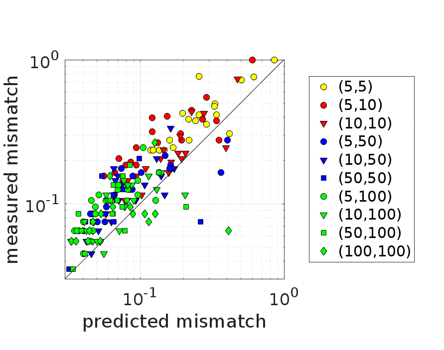
Figure 7: Measured mismatches between the true injected signal and that reconstructed by BayesWave, compared to a first-principles estimate of the lowest achievable mismatch. The measured mismatches are in broad agreement with the first-principles estimate, but are typically 50% higher. The mismatches are smallest for the smallest time-frequency volume signals (high-mass systems), and largest for the largest time-frequency volume signals (low-mass systems) for which BayesWave is unable to reconstruct the full signal. [For visual clarity, we do not show the error bars on the measured mismatches.]

4 Summary and conclusions

We have performed an in-depth analysis of the parameter estimation capabilities of BayesWave, an algorithm for the reconstruction of GW signals without reference to a specific signal model. Using simulated BBH signals added to simulated Advanced LIGO and Advanced Virgo data, we evaluated BayesWave in three key areas: sky position estimation, signal/glitch discrimination, and waveform reconstruction, comparing its performance to first-principles estimates. We found that BayesWave’s effectiveness depends mainly on the time-frequency content of the signal: the fewer wavelets needed to reconstruct a signal, the better the performance. Specifically, higher mass BBH systems tend to have shorter waveforms which can be accurately reconstructed with a small number ($<10$) wavelets.

BayesWave localises the source on the sky better than timing-only triangulation in all scenarios, and is outperformed by optimal Bayesian matched-filter analyses only for low-mass systems ($\leq 50\mathrm{M}_{\odot}$). The measured log Bayes factor for signal-glitch classification closely follows analytic predictions based on the waveform match accuracy and the coherent network SNR. As a result, low time-frequency volume signals are distinguishable from noise glitches provided SNR$>5$–$6$ in all detectors, and high time-frequency volume signals at SNR$>7$–$8$, at a false-alarm rate of 1/100y. Finally, the match between reconstructed and injected waveforms depends on the SNR and the time-frequency volume over which it is spread. Low time-frequency volume signals can achieve matches above 0.9, while high time-frequency volume signals are more typically around a match of $0.6$–$0.8$. The main limitation for waveform reconstruction is the inability to reconstruct the full signal when its SNR is spread over a large number of pixels, rather than noise contamination of the reconstructed signal.

While our study used BBH signals, a key strength of the BayesWave pipeline is that its performance does not depend on signal morphology, so we expect to achieve similar results for generic unmodelled GW transients. For example, it would be very interesting to assess the performance of waveform reconstruction for signals from the post-merger remnant from binary neutron star systems [61], given the recent detection of GW170817 [6]. Also, the waveforms used in our study [48] do not include spin, eccentricity, or higher-mode contributions for BBH signals. While these effects require substantial changes to waveform modelling and matched-filter analyses, BayesWave should be able to account for all of these effects automatically without modification.

Acknowledgements. This work was supported by STFC grants ST/L000962/1 and ST/N005430/1, and by European Research Council Consolidator Grant 647839. We wish to thank Tyson Littenberg, Neil Cornish, and the LIGO-Virgo collaboration Burst group for helpful discussions. We also thank Christopher Berry, Thomas Dent, Jonah Kanner, and Meg Millhouse for useful comments on a draft of this work.

References

- [1] Abbott B P et al. (Virgo, LIGO Scientific) 2016 Phys. Rev. Lett. 116 061102 (Preprint 1602.03837)
- [2] Abbott B P et al. (Virgo, LIGO Scientific) 2016 Phys. Rev. Lett. 116 241103 (Preprint 1606.04855)
- [3] Abbott B â et al. (VIRGO, LIGO Scienitific) 2017 Phys. Rev. Lett. 118 221101
- [4] Abbott B P et al. (Virgo, LIGO Scientific) 2017 Astrophys. J. 851 L35 (Preprint 1711.05578)
- [5] Abbott B P et al. (Virgo, LIGO Scientific) 2017 Phys. Rev. Lett. 119 141101 (Preprint 1709.09660)
- [6] Abbott B et al. (Virgo, LIGO Scientific) 2017 Phys. Rev. Lett. 119 161101 (Preprint 1710.05832)
- [7] Abbott B P et al. (Virgo, LIGO Scientific) 2016 Astrophys. J. 818 L22 (Preprint 1602.03846)
- [8] Belczynski K, Holz D E, Bulik T and O’Shaughnessy R 2016 Nature 534 512 (Preprint 1602.04531)
- [9] Belczynski K et al. 2017 (Preprint 1706.07053)
- [10] Stevenson S, Vigna-Gomez A, Mandel I, Barrett J W, Neijssel C J, Perkins D and de Mink S E 2017 Nature Commun. 8 14906 (Preprint 1704.01352)
- [11] Abbott B P et al. (Virgo, LIGO Scientific) 2016 Phys. Rev. Lett. 116 221101 (Preprint 1602.03841)
- [12] Abbott B P et al. (Virgo, LIGO Scientific) 2016 Phys. Rev. Lett. 116 241102 (Preprint 1602.03840)
- [13] Ott C D 2009 Class. Quant. Grav. 26 063001 (Preprint 0809.0695)
- [14] Kotake K, Takiwaki T, Suwa Y, Nakano W I, Kawagoe S, Masada Y and Fujimoto S i 2012 Adv. Astron. 2012 428757 (Preprint 1204.2330)
- [15] Yakunin K N, Mezzacappa A, Marronetti P, Lentz E J, Bruenn S W, Hix W R, Bronson Messer O E, Endeve E, Blondin J M and Harris J A 2017 (Preprint 1701.07325)
- [16] Richers S, Ott C D, Abdikamalov E, O’Connor E and Sullivan C 2017 Phys. Rev. D95 063019 (Preprint 1701.02752)
- [17] Kuroda T, Kotake K and Takiwaki T 2016 Astrophys. J. 829 L14 (Preprint 1605.09215)
- [18] Bauswein A and Janka H T 2012 Phys. Rev. Lett. 108 011101 (Preprint 1106.1616)
- [19] Hotokezaka K, Kiuchi K, Kyutoku K, Muranushi T, Sekiguchi Y i, Shibata M and Taniguchi K 2013 Phys. Rev. D88 044026 (Preprint 1307.5888)
- [20] Kastaun W and Galeazzi F 2015 Phys. Rev. D91 064027 (Preprint 1411.7975)
- [21] Takami K, Rezzolla L and Baiotti L 2015 Phys. Rev. D91 064001 (Preprint 1412.3240)
- [22] Bernuzzi S, Radice D, Ott C D, Roberts L F, Moesta P and Galeazzi F 2016 Phys. Rev. D94 024023 (Preprint 1512.06397)
- [23] Bernuzzi S, Dietrich T and Nagar A 2015 Phys. Rev. Lett. 115 091101 (Preprint 1504.01764)
- [24] Rezzolla L and Takami K 2016 Phys. Rev. D93 124051 (Preprint 1604.00246)
- [25] Shibata M and Kiuchi K 2017 Phys. Rev. D95 123003 (Preprint 1705.06142)
- [26] Thompson C and Duncan R C 1995 MNRAS 275 255–300
- [27] Ioka K 2001 MNRAS 327 639–662 (Preprint astro-ph/0009327)
- [28] Corsi A and Owen B J 2011 Phys.Rev.D 83 104014 (Preprint 1102.3421)
- [29] Klimenko S, Yakushin I, Mercer A and Mitselmakher G 2008 Class. Quant. Grav. 25 114029 (Preprint 0802.3232)
- [30] Klimenko S, Vedovato G, Drago M, Salemi F, Tiwari V, Prodi G A, Lazzaro C, Ackley K, Tiwari S, Da Silva C F and Mitselmakher G 2016 Phys. Rev. D93 042004 (Preprint 1511.05999)
- [31] Lynch R, Vitale S, Essick R, Katsavounidis E and Robinet F 2017 Phys. Rev. D95 104046 (Preprint 1511.05955)
- [32] Abbott B P et al. (VIRGO, LIGO Scientific) 2016 Phys. Rev. D93 042005 (Preprint 1511.04398)
- [33] Sutton P J et al. 2010 New J. Phys. 12 053034 (Preprint 0908.3665)
- [34] Was M, Sutton P J, Jones G and Leonor I 2012 Phys. Rev. D86 022003 (Preprint 1201.5599)
- [35] Cornish N J and Littenberg T B 2015 Class. Quant. Grav. 32 135012 (Preprint 1410.3835)
- [36] Abbott B P et al. (Virgo, LIGO Scientific) 2016 Phys. Rev. D93 122004 [Addendum: Phys. Rev. D94, 069903 (2016)] (Preprint 1602.03843)
- [37] Klimenko S, Vedovato G, Drago M, Mazzolo G, Mitselmakher G, Pankow C, Prodi G, Re V, Salemi F and Yakushin I 2011 Phys. Rev. D83 102001 (Preprint 1101.5408)
- [38] Abbott B P et al. (VIRGO, LIGO Scientific) 2012 Astron. Astrophys. 539 A124 (Preprint 1109.3498)
- [39] Essick R, Vitale S, Katsavounidis E, Vedovato G and Klimenko S 2015 Astrophys. J. 800 81 (Preprint 1409.2435)
- [40] Becsy B, Raffai P, Cornish N J, Essick R, Kanner J, Katsavounidis E, Littenberg T B, Millhouse M and Vitale S 2017 Astrophys. J. 839 15 [Astrophys. J.839,15(2017)] (Preprint 1612.02003)
- [41] Hooper S, Chung S K, Luan J, Blair D, Chen Y and Wen L 2012 Phys. Rev. D86 024012 (Preprint 1108.3186)
- [42] Littenberg T B and Cornish N J 2015 Phys. Rev. D91 084034 (Preprint 1410.3852)
- [43] Abbott B P et al. (VIRGO, LIGO Scientific) 2017 Phys. Rev. Lett. 118 221101 (Preprint 1706.01812)
- [44] Abbott B P et al. (Virgo, LIGO Scientific) 2017 Phys. Rev. Lett. 119 141101 (Preprint 1709.09660)
- [45] Kanner J B, Littenberg T B, Cornish N, Millhouse M, Xhakaj E, Salemi F, Drago M, Vedovato G and Klimenko S 2016 Phys. Rev. D93 022002 (Preprint 1509.06423)
- [46] Littenberg T B, Kanner J B, Cornish N J and Millhouse M 2016 Phys. Rev. D94 044050 (Preprint 1511.08752)
- [47] Dominik M, Berti E, O’Shaughnessy R, Mandel I, Belczynski K, Fryer C, Holz D E, Bulik T and Pannarale F 2015 Astrophys. J. 806 263 (Preprint 1405.7016)
- [48] Ajith P et al. 2011 Phys. Rev. Lett. 106 241101 (Preprint 0909.2867)
- [49] Sutton P J 2013 (Preprint 1304.0210)
- [50] Fairhurst S 2009 New J. Phys. 11 123006 [Erratum: New J. Phys. 13, 069602 (2011)] (Preprint 0908.2356)
- [51] Fairhurst S 2011 Class. Quant. Grav. 28 105021 (Preprint 1010.6192)
- [52] Fairhurst S 2014 J. Phys. Conf. Ser. 484 012007 (Preprint 1205.6611)
- [53] Fairhurst S 2017 (Preprint 1712.04724)
- [54] Grover K, Fairhurst S, Farr B F, Mandel I, Rodriguez C, Sidery T and Vecchio A 2014 Phys. Rev. D89 042004 (Preprint 1310.7454)
- [55] Berry C P L et al. 2015 Astrophys. J. 804 114 (Preprint 1411.6934)
- [56] Abbott B P et al. (Virgo, LIGO Scientific) 2016 Class. Quant. Grav. 33 134001 (Preprint 1602.03844)
- [57] Chatterji S, Lazzarini A, Stein L, Sutton P J, Searle A and Tinto M 2006 Phys. Rev. D74 082005 (Preprint gr-qc/0605002)
- [58] Veitch J and Vecchio A 2010 Phys. Rev. D81 062003 (Preprint 0911.3820)
- [59] Isi M, Smith R, Vitale S, Massinger T J, Kanner J and Vajpeyi A 2018 (Preprint 1803.09783)
- [60] Sutton P 2018 in preparation
- [61] Abbott B P et al. (Virgo, LIGO Scientific) 2017 Astrophys. J. 851 L16 (Preprint 1710.09320)