X-Pipeline: An analysis package for autonomous gravitational-wave burst searches

Abstract

Autonomous gravitational-wave searches – fully automated analyses of data that run without human intervention or assistance – are desirable for a number of reasons. They are necessary for the rapid identification of gravitational-wave burst candidates, which in turn will allow for follow-up observations by other observatories and the maximum exploitation of their scientific potential. A fully automated analysis would also circumvent the traditional “by hand” setup and tuning of burst searches that is both labourious and time consuming. We demonstrate a fully automated search with X-Pipeline, a software package for the coherent analysis of data from networks of interferometers for detecting bursts associated with GRBs and other astrophysical triggers. We discuss the methods X-Pipeline uses for automated running, including background estimation, efficiency studies, unbiased optimal tuning of search thresholds, and prediction of upper limits. These are all done automatically via Monte Carlo with multiple independent data samples, and without requiring human intervention. As a demonstration of the power of this approach, we apply X-Pipeline to LIGO data to compute the sensitivity to gravitational-wave emission associated with GRB 031108. We find that X-Pipeline is sensitive to signals approximately a factor of 2 weaker in amplitude than those detectable by the cross-correlation technique used in LIGO searches to date. We conclude with the status of running X-Pipeline as a fully autonomous, near real-time triggered burst search in the current LSC-Virgo Science Run.

I Introduction

Gravitational-wave bursts (GWBs) are one of the most interesting classes of signals being sought by the new generation of gravitational-wave detectors. Possible sources include core-collapse supernovae Ott (2009), the merger of binaries containing black-holes or neutron-stars Cutler et al. (1993), gamma-ray bursts Mészáros (2006), and other relativistic systems; see Cutler and Thorne (2002) for a brief overview. These systems typically involve matter at neutron-star densities and very strong gravitational fields, making GWBs potentially rich sources of information on relativistic astrophysics.

The maximum exploitation of a GWB detection would occur when the system is observed by other “messengers” besides gravitational waves, such as in optical, gamma rays, or neutrinos Bloom et al. (2009). Indeed, the first detection of a GWB might rely on independent confirmation by other observatories, and efforts are underway to develop collaborations between gravitational-wave detectors, electromagnetic telescopes, and neutrino observatories (see for example Kanner et al. (2008); Van Elewyck et al. (2009)). The rapid and confident identification of candidate GWBs by gravitational-wave detectors will be vital for these efforts.

Unfortunately, the analysis of gravitational-wave data tends to be a slow process, with a typical latency of several years between the collection of the data and the publication of results. For example, searches for gravitational-wave transients in the first year (2005-2006) of the LIGO Science Run 5 / Virgo Science Run 1 (S5-VSR1) have only recently been published Abbott et al. (2009a, b). One of fastest such analyses has been the search for a gravitational-wave signal associated with GRB 070201 Abbott et al. (2008a), which was published 9 months after the event.

The rapid analysis of gravitational-wave data is not trivial, particularly given the non-stationary nature of the background noise in gravitational-wave detectors and the lack of accurate and comprehensive waveform models for GWB signals. Specifically, we need methods capable of detecting weak signals with a priori unknown waveforms, yet which are simultaneously insensitive to the background noise “glitches” that are common in data from gravitational-wave detectors. Glitch rejection is particularly important since it is the limiting factor in the sensitivity of current burst searches, and a confident detection of a GWB will depend critically on robust background estimation. Detector characterisation Blackburn et al. (2008); Leroy (2009) and search optimization tend to be laborious and time-consuming, as is accounting for other systematic effects such as uncertainties in detector calibration.

These considerations motivate the deployment of data analysis packages that can process data rapidly, yet comprehensively. The ideal scenario is a fully autonomous search – one that runs continuously and without human intervention. This requires an analysis that is self-tuning, adjusting search parameters to changes in the detector network and accounting for variations in the properties of the background noise around the time of candidate events.

We present X-Pipeline Xpi ; Chatterji et al. (2006), a software package designed for autonomous searches for unmodelled gravitational-wave bursts. X-Pipeline targets GWBs associated with external astrophysical “triggers” such as gamma-ray bursts (GRBs), and has been used to search for GWBs associated with more than 100 GRBs that were observed during S5-VSR1 Abbott et al. (2010). It performs a fully coherent analysis of data from arbitrary networks of gravitational-wave detectors, while being robust against noise-induced glitches. We emphasize the novel features of X-Pipeline, particularly a procedure for automated tuning of the background rejection tests. This allows the analysis of each external trigger to be optimized independently, based on background noise characteristics and detector performance at the time of the trigger, maximizing the search sensitivity and the chances of making a detection. This tuning uses independent data samples for tuning and estimating the significance of candidate events, for unbiased selection of GWB candidates. (See also Cannon (2008) for a Bayesian-inspired technique for automated tuning.) X-Pipeline can also account automatically for effects like uncertainty in the sky position of astrophysical trigger and detector calibration uncertainties. Furthermore, for the ongoing S6-VSR2 run, we are preparing the next step in the evolution of GWB searches: a fully autonomous search, wherein X-Pipeline is triggered automatically by email reports of GRBs, and wherein data is analysed and candidate GWBs identified without human intervention. Our goal is the complete analysis of each GRB within 24 hours of the receipt of the GRB notice. Such a rapid analysis would be fast enough to allow further follow-up observations to be prompted by the GWB candidate.

We begin in Section II with a brief discussion of the theory of coherent analysis in gravitational-wave burst detection. In Section III we discuss the main steps followed in an X-Pipeline triggered coherent search. In Section IV we demonstrate the sensitivity of X-Pipeline on GRB 031108 using actual LIGO data, and compare to the upper limits set by the cross-correlation technique used in the published LIGO search for gravitational waves associated with the same GRB. In Section V we discuss the status of autonomous running of X-Pipeline during the current S6-VSR2 science run of LIGO and Virgo. We conclude with a few brief comments in Section VI.

II Coherent Analysis for Gravitational-Wave Burst Detection

Most algorithms currently used in gravitational-wave burst detection can be grouped into two broad classes. In incoherent methods Anderson et al. (2001); Sylvestre (2002), candidate events typically are constructed from each detector data stream independently, and one looks for events with similar duration and frequency band that occur in all detectors simultaneously. By contrast, coherent methods Gursel and Tinto (1989); Tinto (1996); Flanagan and Hughes (1998); Anderson et al. (2001); Sylvestre (2003); Cadonati (2004); Wen and Schutz (2005); Klimenko et al. (2005, 2006); Mohanty et al. (2006); Rakhmanov (2006); Chatterji et al. (2006); Summerscales et al. (2008); Hayama et al. (2007); Searle et al. (2008, 2009); Klimenko et al. (2008) combine data from multiple detectors before processing, and create a single list of candidate events for the whole network. Coherent methods have some advantages over incoherent methods, such as demonstrated usefulness in rejecting background noise “glitches” Cadonati (2004); Wen and Schutz (2005); Chatterji et al. (2006), and for reconstructing GWB waveforms Gursel and Tinto (1989); Summerscales et al. (2008). A less-recognized advantage of coherent methods is that they are relatively easy to tune. For example, time-frequency coincidence windows for comparing candidate GWBs in different detectors are not necessary. Detectors are naturally weighted by their relative sensitivity, so there is no need to tune the relative thresholds for generating candidate events in each detector. This ease of tuning makes coherent methods particularly useful for rapid searches.

That said, there are also draw-backs to coherent methods, the most significant being computational cost. Coherent combinations are typically a function of the sky position of the GWB source; there are $\gtrsim 10^{3}$ resolvable directions on the sky for a worldwide detector network Fairhurst (2009). This cost is compounded by the need to estimate the background due to noise, which requires repeated re-analysis of the data using time shifts. Fortunately, in triggered searches the sky position of the source is often known to high accuracy, and the amount of data to be analysed is relatively small (typically hours), so the computational cost of a fully coherent analysis is modest. This allows triggered searches to take advantage of the benefits of coherent methods while avoiding or minimizing most of the drawbacks.

In this section we give a brief review of some of the main principles of coherent network analysis as implemented in X-Pipeline.

II.1 Formulation

A rigorous treatment of gravitational waves is based on linearized perturbations of the spacetime metric around a fixed background (see for example Flanagan and Hughes (2005)). In the linearized theory based on flat spacetime, when working in a suitable gauge, the perturbations representing the gravitational waves can be shown to obey the ordinary wave equation. The gravitational waves are transverse, and travel at the speed of light. They have two independent polarizations, commonly referred to as “plus” ($+$) and “cross” ($\times$). Their physical manifestation is a quadrupolar change in the distance between freely falling test particles (approximated in interferometric gravitational-wave detectors by the mirrors in the interferometer arms). Explicit definitions of the plus and cross polarization states can be found, for example, in Anderson et al. (2001).

The interferometers currently used to try to detect these waves are based on a laser, beamsplitter, and mirrors at the ends of each arm which serve as test masses. Data from each interferometer record the length difference of the arms and, when calibrated, measure the strain induced by a gravitational wave. The LIGO detectors are kilometer-scale power-recycled Michelson interferometers with orthogonal Fabry-Perot arms (Abbott et al., 2004, 2009c). There are two LIGO observatories: one located at Hanford, WA and the other at Livingston, LA. The Hanford site houses two interferometers: one with 4 km arms (H1), and the other with 2 km arms (H2). The Livingston observatory has one 4 km interferometer (L1). The Virgo detector (V1) is in Cascina near Pisa, Italy. It is a 3 km long power-recycled Michelson interferometer with orthogonal Fabry-Perot arms (Acernese et al., 2008). The GEO 600 detector (Grote et al., 2008), located near Hannover, Germany, is also operational, though with a lower sensitivity than LIGO and Virgo. These instruments are all designed to detect gravitational waves with frequencies ranging from $\sim 30$ Hz to several kHz.

Consider a gravitational wave $h_{+}(t,\vec{x}),h_{\times}(t,\vec{x})$ from a direction $\hat{\Omega}$. The output of detector $\alpha\in[1,\ldots,D]$ is a linear combination of this signal and noise $n_{\alpha}$:

$$d_{\alpha}(t+\Delta t_{\alpha}(\hat{\Omega})) = F_{\alpha}^{+}(\hat{\Omega})h_{+}(t)+F_{\alpha}^{\times}(\hat{\Omega})h_{\times}(t)$$ (1)

$$\mbox{}+n_{\alpha}(t+\Delta t_{\alpha}(\hat{\Omega}))\,.$$

Here $F^{+}(\hat{\Omega})$, $F^{\times}(\hat{\Omega})$ are the antenna response functions describing the sensitivity of the detector to the plus and cross polarizations (note that the choice of polarization basis is arbitrary; we use the $\psi=0$ choice of Appendix B of Anderson et al. (2001)). Also, $\Delta t_{\alpha}(\hat{\Omega})$ is the time delay between the position $\vec{r}_{\alpha}$ of detector $\alpha$ and an arbitrary reference position $\vec{r}_{0}$:

$$\Delta t_{\alpha}(\hat{\Omega})=\frac{1}{c}(\vec{r}_{0}-\vec{r}_{\alpha})\cdot\hat{\Omega}\,.$$ (2)

For brevity, we suppress explicit mention of the time delay and understand the data streams to be time-shifted by the appropriate amount prior to analysis. We also write $h_{+,\times}(t)\equiv h_{+,\times}(t,\vec{r}_{0})$.

Since the detector data is sampled discretely, we use discrete notation henceforth. The discrete Fourier-transform $\tilde{x}[k]$ of a time-series $x[j]$ is

$$\tilde{x}[k] = \sum_{j=0}^{N-1}x[j]\,\mathrm{e}^{-i2\pi jk/N}\,,$$

$$x[j] = \frac{1}{N}\sum_{k=0}^{N-1}\tilde{x}[k]\,\mathrm{e}^{i2\pi jk/N}\,,$$ (3)

where $N$ is the number of data points in the time domain. Denoting the sampling rate by $f_{s}$, we can convert from continuous to discrete notation using $x(t)\to x[j]$, $\tilde{x}(f)\to f_{s}^{-1}\tilde{x}[k]$, $\int dt\to f_{s}^{-1}\sum_{j}$, $\int df\to f_{s}N^{-1}\sum_{k}$, $\delta(t-t^{\prime})\to f_{s}\delta_{jj^{\prime}}$, and $\delta(f-f^{\prime})\to Nf_{s}^{-1}\delta_{kk^{\prime}}$. For example, the one-sided noise power spectral density $S_{\alpha}[k]$ of the noise $\tilde{n}_{\alpha}$ is

$$\langle\tilde{n}_{\alpha}^{*}[k]\tilde{n}_{\beta}[k^{\prime}]\rangle=\frac{N}{2}\delta_{\alpha\beta}\delta_{kk^{\prime}}S_{\alpha}[k]\,,$$ (4)

where the angle brackets indicate an average over noise instantiations.

It is conceptually convenient to define the noise-spectrum-weighted quantities

$$\tilde{d}_{\mathrm{w}\alpha}[k] = \frac{\tilde{d}_{\alpha}[k]}{\sqrt{\frac{N}{2}S_{\alpha}[k]}}\,,$$ (5)

$$\tilde{n}_{\mathrm{w}\alpha}[k] = \frac{\tilde{n}_{\alpha}[k]}{\sqrt{\frac{N}{2}S_{\alpha}[k]}}\,,$$ (6)

$$F^{+,\times}_{\mathrm{w}\alpha}(\hat{\Omega},k) = \frac{F^{+,\times}_{\alpha}(\hat{\Omega})}{\sqrt{\frac{N}{2}S_{\alpha}[k]}}\,.$$ (7)

The normalization of the whitened noise is

$$\langle\tilde{n}_{\mathrm{w}\alpha}^{*}[k]\tilde{n}_{\mathrm{w}\beta}[k^{\prime}]\rangle=\delta_{\alpha\beta}\delta_{kk^{\prime}}\,.$$ (8)

With this notation, equation (1) for the data measured from a set of $D$ detectors can be written in the simple matrix form

$$\boldsymbol{\tilde{d}}=\boldsymbol{F}\boldsymbol{\tilde{h}}+\boldsymbol{\tilde{n}}\,,$$ (9)

where we have dropped the explicit indices for frequency and sky position. We use the boldface symbols $\boldsymbol{\tilde{d}}$, $\boldsymbol{F}$, $\boldsymbol{\tilde{n}}$ to refer to noise-weighted quantities that are vectors or matrices on the space of detectors (note that $\boldsymbol{\tilde{h}}$ is not noise-weighted and is not in the space of the detectors):

$$\boldsymbol{\tilde{d}}\equiv\left[\begin{array}[]{c}\tilde{d}_{\mathrm{w}1}\\ \tilde{d}_{\mathrm{w}2}\\ \vdots\\ \tilde{d}_{\mathrm{w}D}\end{array}\right]\,,\quad\boldsymbol{\tilde{h}}\equiv\left[\begin{array}[]{c}\tilde{h}_{+}\\ \tilde{h}_{\times}\end{array}\right]\,,\quad\boldsymbol{\tilde{n}}\equiv\left[\begin{array}[]{c}\tilde{n}_{\mathrm{w}1}\\ \tilde{n}_{\mathrm{w}1}\\ \vdots\\ \tilde{n}_{\mathrm{w}D}\end{array}\right]\,,$$ (10)

and

$$\boldsymbol{F} \equiv \left[\begin{array}[]{c c}\boldsymbol{F^{+}}&\boldsymbol{F^{\times}}\end{array}\right]\equiv\left[\begin{array}[]{c c}F^{+}_{\mathrm{w}1}&F^{\times}_{\mathrm{w}1}\\ F^{+}_{\mathrm{w}2}&F^{\times}_{\mathrm{w}2}\\ \vdots&\vdots\\ F^{+}_{\mathrm{w}D}&F^{\times}_{\mathrm{w}D}\end{array}\right]\,.$$ (16)

(See Table 1 for a list of the dimensions of all of the quantities used in this section.) Note that each of these quantities is a function of both frequency and (through the antenna response or implied time shift) sky position. As a consequence, coherent combinations typically have to be re-computed for every frequency bin as well as for every sky position. Note also that, because of the noise-spectrum weighting, the whitened noise is isotropically distributed in the space of detectors [equation (8)]. Therefore, all information on the sensitivity of the network both as a function of frequency and of sky position is contained in the matrix $\boldsymbol{F}$ defined by equation (16).

quantity	dimensions
$\boldsymbol{h}$, $\boldsymbol{\tilde{h}}$, $\boldsymbol{\tilde{h}_{\mathrm{max}}}$	$2\times 1$ vectors
$\boldsymbol{F}$	$D\times 2$ matrix
$\boldsymbol{P}^{\text{GW}}$, $\boldsymbol{P}^{\text{null}}$, $\boldsymbol{I}$	$D\times D$ matrices
all other boldfaced symbols: $\boldsymbol{d}$, $\boldsymbol{\tilde{d}}$, $\boldsymbol{F^{+}}$, $\boldsymbol{f}{}^{+}$, $\boldsymbol{e}{}^{+}$ etc.	$D\times 1$ vectors

Table 1: Dimensionality of various quantities used in this section. $D$ is the number of detectors in the network.

II.2 Standard Likelihood

In this section we describe some of the simpler coherent likelihoods: those that can be computed from projections of the data. These are the main ones used for signal detection in X-Pipeline. We begin with the simplest coherent likelihood of all: the standard or maximum likelihood, first derived in Flanagan and Hughes (1998); Anderson et al. (2001).

Let $P(\boldsymbol{\tilde{d}}|\boldsymbol{\tilde{h}})$ be the probability of obtaining the whitened data $\boldsymbol{\tilde{d}}$ in one time-frequency pixel in the presence of a known gravitational wave $\boldsymbol{\tilde{h}}$ from a known direction. Assuming Gaussian noise,

$$P(\boldsymbol{\tilde{d}}|\boldsymbol{\tilde{h}})=\frac{1}{(2\pi)^{D/2}}\exp\left[-\frac{1}{2}\left|\boldsymbol{\tilde{d}}-\boldsymbol{F}\boldsymbol{\tilde{h}}\right|^{2}\right].$$ (17)

For a set $\{\boldsymbol{\tilde{d}}\}$ of $N_{\mathrm{p}}$ time-frequency pixels,

$$P(\{\boldsymbol{\tilde{d}}\}|\{\boldsymbol{\tilde{h}}\})=\frac{1}{(2\pi)^{N_{\mathrm{p}}D/2}}\exp\left[-\frac{1}{2}\sum_{k}\left|\boldsymbol{\tilde{d}}[k]-\boldsymbol{F}[k]\boldsymbol{\tilde{h}}[k]\right|^{2}\right]\,,$$ (18)

where $k$ indexes the pixels. The likelihood ratio $L$ is defined by the log-ratio of this probability to the corresponding probability under the null hypothesis,

$$L\equiv\ln\frac{P(\{\boldsymbol{\tilde{d}}\}|\{\boldsymbol{\tilde{h}}\})}{P(\{\boldsymbol{\tilde{d}}\}|\{0\})}=\frac{1}{2}\sum_{k}\left[\left|\boldsymbol{\tilde{d}}\right|^{2}-\left|\boldsymbol{\tilde{d}}-\boldsymbol{F}\boldsymbol{\tilde{h}}\right|^{2}\right]\,,$$ (19)

where $P(\{\boldsymbol{\tilde{d}}\}|\{0\})$ is the probability of measuring the data $\{\boldsymbol{\tilde{d}}\}$ when no GWB is present ($\boldsymbol{\tilde{h}}=0$).

In practice, the signal waveform $\boldsymbol{\tilde{h}}$ is not known a priori, so it is not clear how to compute the likelihood ratio (19). One approach is to treat the waveform values $\boldsymbol{\tilde{h}}=(\tilde{h}_{+},\tilde{h}_{\times})$ in each time-frequency pixel as free parameters to be fit to the data. The best-fit values $\boldsymbol{\tilde{h}_{\mathrm{max}}}$ are those that maximize the likelihood ratio:

$$0=\left.\frac{\partial L}{\partial\boldsymbol{\tilde{h}}}\right|_{\boldsymbol{\tilde{h}}=\boldsymbol{\tilde{h}_{\mathrm{max}}}}\,.$$ (20)

Because the likelihood ratio $L$ is quadratic in $\boldsymbol{\tilde{h}}$, (20) gives a linear equation for $\boldsymbol{\tilde{h}_{\mathrm{max}}}$. The solution is

$$\boldsymbol{\tilde{h}_{\mathrm{max}}}=(\boldsymbol{F}^{\dagger}\boldsymbol{F})^{-1}\boldsymbol{F}^{\dagger}\,\boldsymbol{\tilde{d}}\,,$$ (21)

where we use $\mbox{}^{\dagger}$ to denote the conjugate transpose. ($\boldsymbol{F}$ is real, but other quantities such as the data vector $\boldsymbol{\tilde{d}}$ are complex.) Substituting the solution for $\boldsymbol{\tilde{h}_{\mathrm{max}}}$ in (19) gives the standard likelihood,

$$E_{\mathrm{SL}}\equiv 2L(\boldsymbol{\tilde{h}_{\mathrm{max}}})=\sum_{k}\boldsymbol{\tilde{d}}^{\dagger}\boldsymbol{P}^{\text{GW}}\boldsymbol{\tilde{d}}\,,$$ (22)

where we define

$$\boldsymbol{P}^{\text{GW}}\equiv\boldsymbol{F}\,(\boldsymbol{F}^{\dagger}\boldsymbol{F})^{-1}\boldsymbol{F}^{\dagger}\,$$ (23)

and we have used the fact that $\boldsymbol{P}^{\text{GW}}$ is Hermitian. (The factor of 2 in the definition of $E_{\mathrm{SL}}$ is purely a matter of taste.)

II.3 Projection Operators and the Null Energy

It is easy to show that $\boldsymbol{P}^{\text{GW}}$ is a projection operator that projects the data into the subspace spanned by $\boldsymbol{F^{+}}$ and $\boldsymbol{F^{\times}}$. We know by equation (1) or (9)-(16) that the contribution to $\boldsymbol{\tilde{d}}$ by any gravitational wave from a fixed sky position is restricted to this subspace. The standard likelihood is therefore the maximum amount of energy in the whitened data that is consistent with the hypothesis of a gravitational wave from a given sky position.

Contrast this with the total energy in the data, which is simply

$${E_{\mathrm{tot}}}=\sum_{k}\left|\boldsymbol{\tilde{d}}\right|^{2}\,.$$ (24)

The total energy is an incoherent statistic in the sense that it contains only autocorrelation terms and no cross-correlation terms. In the limit of a one-detector network, this is the quantity one computes for each time-frequency pixel in an excess-power search Anderson et al. (2001).

The projection operator $\boldsymbol{P}^{\text{null}}\equiv(\boldsymbol{I}-\boldsymbol{P}^{\text{GW}})$, which is orthogonal to $\boldsymbol{P}^{\text{GW}}$, cancels the gravitational-wave signal. This yields the null stream with energy

$${E_{\mathrm{null}}}\equiv{E_{\mathrm{tot}}}-{E_{\mathrm{SL}}}=\sum_{k}\boldsymbol{\tilde{d}}^{\dagger}\boldsymbol{P}^{\text{null}}\boldsymbol{\tilde{d}}\,.$$ (25)

The null energy is the minimum amount of energy in the whitened data that is inconsistent with the hypothesis of a gravitational wave from a given sky position.

One advantage of coherent analysis is that the projection from the full data space with energy ${E_{\mathrm{tot}}}$ to the subspace spanned by $\boldsymbol{F^{+}}$, $\boldsymbol{F^{\times}}$ with energy ${E_{\mathrm{SL}}}$ removes some fraction of the noise, with energy ${E_{\mathrm{null}}}$, without removing any of the signal component (small errors in calibrations, sky position, or power spectra change $\boldsymbol{F}$ but this affects the signal energy only at second order). This means that a signal can be detected with higher confidence. An important caveat is that the full benefit is gained only if the sky position is known a priori, such as in gamma-ray burst searches. If the sky position of the source is not known a priori, one typically repeats the calculation of the likelihood for a set of directions spanning the entire sky ($\gtrsim 10^{3})$ directions). Since $\boldsymbol{F^{+}}$, $\boldsymbol{F^{\times}}$ vary with the sky position, this means that many different projection operators will be applied to the data. This will incur a false-alarm penalty.

II.4 Dominant Polarization Frame and Other Likelihoods

For a single time-frequency pixel, the data from a set of $D$ detectors is a vector in a $D$-dimensional complex space. One basis of this space is formed by the set of single-detector strains (the basis in which all equations have been written thus far); however, this is not the most convenient basis for writing detection statistics. The $2$-dimensional subspace defined by $\boldsymbol{F^{+}},\,\boldsymbol{F^{\times}}$ is a natural starting point for the construction of a better basis. If we examine the properties of this $2$-dimensional space, we find there is a direction (a choice of polarization angle) in which the detector network has the maximum antenna response, and an orthogonal direction in which the network has minimum antenna response. Choosing those two directions as basis vectors, and completing them with an orthonormal basis for the null space, yields a very convenient basis in which to construct detection statistics. To further simplify things it is possible to define the $+,\,\times$ polarizations so that $\boldsymbol{F^{+}}$ lies along the first basis vector, and $\boldsymbol{F^{\times}}$ along the second. This choice of polarization definition is called the dominant polarization frame or DPF Klimenko et al. (2005, 2006). Note that while searches for modeled signals such as binary inspirals often select the polarization basis with reference to the source, the DPF polarization basis is tailored to the detector network at each frequency. This makes it a particularly convenient choice when searching for more general gravitational-wave burst signals.

To see how one constructs the DPF, recall that the antenna response vectors in two frames separated by a polarization angle $\psi$ are related by

$$\boldsymbol{F^{+}}(\psi) = \cos 2\psi\boldsymbol{F^{+}}(0)+\sin 2\psi\boldsymbol{F^{\times}}(0)\,,$$ (26)

$$\boldsymbol{F^{\times}}(\psi) = -\sin 2\psi\boldsymbol{F^{+}}(0)+\cos 2\psi\boldsymbol{F^{\times}}(0)\,$$ (27)

(see for example equations (B9), (B10) of Anderson et al. (2001)). It is straightforward to show that for any direction on the sky, one can always chose a polarization frame such that $\boldsymbol{F^{+}}(\psi)$ and $\boldsymbol{F^{\times}}(\psi)$ are orthogonal and $|\boldsymbol{F^{+}}(\psi)|>|\boldsymbol{F^{\times}}(\psi)|$. Explicitly, given $\boldsymbol{F^{+}}(0)$, $\boldsymbol{F^{\times}}(0)$ in the original polarization frame, the rotation angle $\psi_{\mathrm{DP}}$ giving the dominant polarization frame is

$$\psi_{DP}(\hat{\Omega},k) = \frac{1}{4}\mathrm{atan2}\left(2\boldsymbol{F^{+}}(0)\cdot\boldsymbol{F^{\times}}(0),\right.$$ (28)

$$\left.\quad|\boldsymbol{F^{+}}(0)|^{2}-|\boldsymbol{F^{\times}}(0)|^{2}\right)\,.$$

where $\mathrm{atan2}(y,x)$ is the arctangent function with range $(-\pi,\pi]$. Note that $\psi_{DP}$ is a function of both sky position and frequency (through the noise weighting of $\boldsymbol{F^{+}}$ and $\boldsymbol{F^{\times}}$).

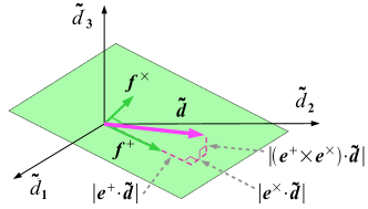
We denote the antenna response vectors in the DPF by the lower-case symbols $\boldsymbol{f}{}^{+}$, $\boldsymbol{f}{}^{\times}$. They have the properties

$$|\boldsymbol{f}{}^{+}|^{2}\geq|\boldsymbol{f}{}^{\times}|^{2}\,,$$ (29)

$$\boldsymbol{f}{}^{+}\cdot\boldsymbol{f}{}^{\times}=0\,.$$ (30)

In the DPF the unit vectors $\boldsymbol{e}{}^{+}\equiv\boldsymbol{f}{}^{+}/|\boldsymbol{f}{}^{+}|$, $\boldsymbol{e}{}^{\times}\equiv\boldsymbol{f}{}^{\times}/|\boldsymbol{f}{}^{\times}|$ are part of an orthonormal coordinate system; see Figure 1. Indeed, the DPF can be viewed as the natural coordinate system in the space of detector data for understanding the sensitivity of the network. Mathematically, rotating to the DPF is the same as doing a singular value decomposition of the matrix $\boldsymbol{F}$. The singular values are $|\boldsymbol{f}{}^{+}|^{2}$ and $|\boldsymbol{f}{}^{\times}|^{2}$; i.e., the magnitudes of the antenna response evaluated in the DPF.

Figure 1: Space of detector strains for the 3-detector case for one data sample. The green plane is the plane spanned by the antenna response vectors $\boldsymbol{f}{}^{+}$, $\boldsymbol{f}{}^{+}$. The thick magenta line is the vector of detector strains $\boldsymbol{\tilde{d}}$ for one realization of noise and signal. The dashed lines show the projection of the data vector into the detector response plane and into the null space.

It should be noted that the DPF does not specify any particular choice of basis for the null space. Convenient choices for the null basis can be motivated by how the null energy is used in the search, but we do not consider this issue here.

In the DPF, the projection operator $\boldsymbol{P}^{\text{GW}}$ takes on the very simple form

$$\boldsymbol{P}^{\text{GW}}=\boldsymbol{e}{}^{+}\boldsymbol{e}{}^{+}{}^{\dagger}+\boldsymbol{e}{}^{\times}\boldsymbol{e}{}^{\times}{}^{\dagger}~{}.$$ (31)

The standard likelihood (22) becomes

$${E_{\mathrm{SL}}}=\sum_{k}\left[\left|\boldsymbol{e}{}^{+}\cdot\boldsymbol{\tilde{d}}\right|^{2}+\left|\boldsymbol{e}{}^{\times}\cdot\boldsymbol{\tilde{d}}\right|^{2}\right]\,,$$ (32)

where we use the notation $\boldsymbol{a}\cdot\boldsymbol{b}$ to denote the familiar dot product between $D\times 1$ dimensional vectors $\boldsymbol{a}$ and $\boldsymbol{b}$. The plus energy or hard constraint likelihood Klimenko et al. (2005, 2006) is the energy in the ${h_{+}}$ polarization in the DPF:

$${E_{+}}\equiv\sum_{k}\left|\boldsymbol{e}{}^{+}\cdot\boldsymbol{\tilde{d}}\right|^{2}\,.$$ (33)

The cross energy is defined analogously:

$${E_{\times}}\equiv\sum_{k}\left|\boldsymbol{e}{}^{\times}\cdot\boldsymbol{\tilde{d}}\right|^{2}\,.$$ (34)

The soft constraint likelihood Klimenko et al. (2005, 2006) (not a projection likelihood) is

$${E_{\mathrm{soft}}}\equiv\sum_{k}\left[\left|\boldsymbol{e}{}^{+}\cdot\boldsymbol{\tilde{d}}\right|^{2}+\epsilon\left|\boldsymbol{e}{}^{\times}\cdot\boldsymbol{\tilde{d}}\right|^{2}\right]\,,$$ (35)

where the weighting factor $\epsilon$ is defined in the DPF as

$$\epsilon\equiv\frac{\left|\boldsymbol{f}{}^{\times}\right|^{2}}{\left|\boldsymbol{f}{}^{+}\right|^{2}}\in[0,1]\,.$$ (36)

Typical values are $\epsilon\sim 0.01-0.1$ for the LIGO network.

Numerous other likelihood-based coherent statistics have been introduced in the literature, such as the Tikhonov regularized statistic Rakhmanov (2006), a sky-map variability statistic Hayama et al. (2007), and modified constraint likelihood statistics Klimenko et al. (2008). Also, comprehensive Bayesian formulations of the problem of GWB detection and waveform estimation are described in Summerscales et al. (2008); Searle et al. (2008, 2009). While some of these statistics are available in X-Pipeline, we do not consider them here.

II.5 Statistical Properties

One convenient property of the projection likelihoods ${E_{+}}$, ${E_{\times}}$, ${E_{\mathrm{SL}}}$, ${E_{\mathrm{null}}}$, ${E_{\mathrm{tot}}}$ is that their statistical properties for signals in Gaussian background noise are very simple. Specifically, for a set of time-frequency pixels and a sky position chosen a priori, each of these energies follows a $\chi^{2}$ distribution with $2N_{\mathrm{p}}D_{\mathrm{proj}}$ degrees of freedom:

$$2E\sim\chi^{2}_{2N_{\mathrm{p}}D_{\mathrm{proj}}}(\lambda)\,.$$ (37)

Here $N_{\mathrm{p}}$ is the number of pixels (or time-frequency volume). $D_{\mathrm{proj}}$ is the number of dimensions of the projection, which is 1 for ${E_{+}},{E_{\times}}$, 2 for ${E_{\mathrm{SL}}}$, and $D$ for ${E_{\mathrm{tot}}}$. $D_{\mathrm{proj}}=D-2$ for ${E_{\mathrm{null}}}$, except when the null stream is constructed as the difference of the data streams from the two co-aligned LIGO-Hanford detectors, H1 and H2, in which case it is $D-1$ (the H1-H2 sub-network is only sensitive to a single gravitational-wave polarization, so only one dimension is removed in forming the null stream). The factor of 2 in the degrees of freedom occurs because the data are complex. The non-centrality parameter $\lambda$ is the expected squared signal-to-noise ratio of a matched filter for the waveform restricted to the time-frequency region in question and after projection by the appropriate likelihood projection operator, summed over the network:

$$\lambda_{+} = 2\sum_{k}|\boldsymbol{f}{}^{+}|^{2}|{h_{+}}|^{2}$$ (38)

$$= \frac{4}{N}\sum_{\alpha}\sum_{k}\frac{\left|F^{+}_{\alpha}(\psi_{DP})\tilde{h}_{+}[k](\psi_{DP})\right|^{2}}{S_{\alpha}[k]}=:\rho_{+}^{2},$$

$$\lambda_{\times} = 2\sum_{k}|\boldsymbol{f}{}^{\times}|^{2}|{h_{\times}}|^{2}$$ (39)

$$= \frac{4}{N}\sum_{\alpha}\sum_{k}\frac{\left|F^{\times}_{\alpha}(\psi_{DP})\tilde{h}_{\times}[k](\psi_{DP})\right|^{2}}{S_{\alpha}[k]}=:\rho_{\times}^{2},\qquad$$

$$\lambda_{\mathrm{SL}} = 2\sum_{k}\left[|\boldsymbol{f}{}^{+}|^{2}|{h_{+}}|^{2}+|\boldsymbol{f}{}^{\times}|^{2}|{h_{\times}}|^{2}\right]$$ (40)

$$= \frac{4}{N}\sum_{\alpha}\sum_{k}\frac{\left|F^{+}_{\alpha}\tilde{h}_{+}[k]+F^{\times}_{\alpha}\tilde{h}_{\times}[k]\right|^{2}}{S_{\alpha}[k]}=:\rho^{2}\,,$$

$$\lambda_{\mathrm{tot}}\!\! = \rho^{2}\,,$$ (41)

$$\lambda_{\mathrm{null}}\!\!\! = 0\,.$$ (42)

Note that in (38) and (39) the antenna responses and waveforms are defined in the DPF. Eqn. (40) is actually independent of the polarization basis used.

The mean and standard deviation of the non-central $\chi^{2}$ distribution (37) are $(2N_{\mathrm{p}}D_{\mathrm{proj}}+\lambda)$ and $\sqrt{2N_{\mathrm{p}}D_{\mathrm{proj}}}$. Consequently, one expects a signal to be detectable by a given coherent statistic when

$$\frac{\lambda}{\sqrt{2N_{\mathrm{p}}D_{\mathrm{proj}}}}\gg 1\,.$$ (43)

Table 2 shows the mean and standard deviation of various energy measures when the correct sky position and the time-frequency region are known a priori.

For a circularly polarized or unpolarized gravitational wave, $\rho_{\times}^{2}/\rho_{+}^{2}\simeq\epsilon\ll 1$ for typical sky positions. For example, for the LIGO-Virgo network of detectors H1-H2-L1-V1, assuming H2 is half as sensitive as H1, L1, and V1, the median value of $\epsilon$ is 0.1, while for the LIGO network H1-H2-L1 the median is 0.02. As a consequence, for many signals $\rho_{\times}^{2}$ is negligible. (An exception is linearly polarized GWBs; for these the random polarization angle can make $\rho_{\times}^{2}>\rho_{+}^{2}$ in the H1-H2-L1 network for approximately 10% of signals for a typical sky position.) Since all of the energies except ${E_{\times}}$ in Table 2 include $\rho_{+}^{2}$, their relative performance is dominated by the level of noise fluctuations. The noise fluctuations in the energies scale as the square-root of the number of orthogonal directions used to compute the energy. As a consequence, we expect those statistics that project the data down to fewer dimensions to perform better for GWB detection. For ${E_{+}}$ the data is projected onto a single direction. ${E_{\mathrm{SL}}}$ and ${E_{\mathrm{soft}}}$ use data along two directions, and so have higher noise. The total energy ${E_{\mathrm{tot}}}$ uses all of the data and therefore incorporates the largest contributions from noise. In practice, coherent consistency tests (discussed in the next section) can be used to reduce the noise background, allowing statistics like ${E_{\mathrm{SL}}}$ to be used effectively, so that all of the signal-to-noise ratio of a GWB ($\rho_{+}^{2}$ and $\rho_{\times}^{2}$) can be included in the detection statistic.

Energy measure	$\mathrm{mean}(2E)|_{\mathrm{GWB}}$	$\displaystyle{\frac{\mathrm{std}(2E)|_{\mathrm{noise}}}{\sqrt{2N_{\mathrm{p}}}}}$
$E_{\mathrm{TOT}}$	$\rho^{2}=\rho_{+}^{2}+\rho_{\times}^{2}$	$\sqrt{D}$
$E_{\mathrm{SL}}$	$\rho^{2}=\rho_{+}^{2}+\rho_{\times}^{2}$	$\sqrt{2}$
$E_{\mathrm{+}}$	$\rho_{+}^{2}$	1
$E_{\mathrm{\times}}$	$\rho_{\times}^{2}$	1
$E_{\mathrm{soft}}$	$\simeq(\rho_{+}^{2}+\epsilon\rho_{\times}^{2})$	$\sqrt{1+\epsilon}$

Table 2: Expected signal and noise contributions to various coherent energies. The mean($2E$) column shows the contribution to the mean energy due to a gravitational wave, evaluated in the dominant polarization frame. See equations (36), (38)–(41). The std($2E$) column shows the standard deviation due to noise fluctuations assuming a non-aligned detector network (i.e., $|\boldsymbol{f}{}^{\times}|>0$). The values for ${E_{\mathrm{soft}}}$ are written as approximate because the weighting factor $\epsilon$ is itself a function of frequency. All of these values assume the time-frequency region to sum over and the correct sky location are known a priori.

II.6 Incoherent Energies and Background Rejection

The various likelihood measures ${E_{\mathrm{SL}}}$, ${E_{+}}$, etc. are motivated as detection statistics under the assumption of stationary Gaussian background noise. Real detectors do not have purely Gaussian noise. Rather, real detector noise contains glitches, which are short transients of excess strain that can masquerade as gravitational-wave burst signals. In practice, without a means to distinguish noise glitches from true GW signals, the sensitivity of a burst search will be limited by such glitches. Coherent analyses can be particularly susceptible to such false alarms, since even a glitch in a single detector will produce large values for likelihoods such as ${E_{\mathrm{SL}}}$. In this section we outline a technique for the effective suppression of such false alarms in coherent analyses.

As shown in Chatterji et al. Chatterji et al. (2006), one can use the autocorrelation component of coherent energies to construct tests that are effective at rejecting glitches. This coherent veto test is based on the null space – the subspace orthogonal to that used to define the standard likelihood. The projection of $\boldsymbol{d}$ on this subspace contains only noise, and the presence or absence of GWs should not affect this projection in any way. By contrast, glitches do not couple into the data streams with any particular relationship to $\boldsymbol{F^{+}},\boldsymbol{F^{\times}}$. As a result, glitches will generally be present in the null space projection. This provides a way to distinguish true GWs from glitches, by requiring the null energy to be small for a transient to be considered a GW Wen and Schutz (2005).

To see how an effective test can be constructed, note that we can write equation (25) for the null energy as

$${E_{\mathrm{null}}} = \sum_{k}\sum_{\alpha,\beta}\tilde{d}^{\dagger}_{\alpha}P^{\mathrm{null}}_{\alpha\beta}\tilde{d}^{\vphantom{\dagger}}_{\beta}\,.$$ (44)

As pointed out in Chatterji et al. Chatterji et al. (2006), the null energy is composed of cross-correlation terms $\tilde{d}^{\dagger}_{\alpha}\tilde{d}^{\vphantom{\dagger}}_{\beta}$ and auto-correlation terms $\tilde{d}^{\dagger}_{\alpha}\tilde{d}^{\vphantom{\dagger}}_{\alpha}$. If the transient signal is not correlated between detectors (as is expected for glitches), then the cross-correlation terms will be small compared to the auto-correlation terms. As a consequence, for a glitch we expect the null energy to be dominated by the auto-correlation components:

$${E_{\mathrm{null}}}\simeq{I_{\mathrm{null}}}\equiv\sum_{k}\sum_{\alpha}P^{\mathrm{null}}_{\alpha\alpha}|\tilde{d}_{\alpha}|^{2}\,.\qquad\mathrm{(glitches)}$$ (45)

This auto-correlation part of the null energy is called the incoherent energy.

By contrast, for a GW signal, the transient is correlated between the detectors according to equations (1) or (9)–(16). By construction of the null projection operator, these correlations cancel in the null stream, leaving only Gaussian noise. They cannot cancel in ${I_{\mathrm{null}}}$, however, since that is a purely incoherent statistic. Therefore, for a strong GW signal we expect

$${E_{\mathrm{null}}}\ll{I_{\mathrm{null}}}\,.\qquad\mathrm{(GW)}$$ (46)

Based on these considerations, the coherent veto test introduced by Chatterji et al. Chatterji et al. (2006) is to keep only transients with

$${I_{\mathrm{null}}}/{E_{\mathrm{null}}}>C,$$ (47)

where $C$ is some constant greater than 1. This test is particularly effective at eliminating large-amplitude glitches. For smaller amplitude glitches ${E_{\mathrm{null}}}$ can be small compared to ${I_{\mathrm{null}}}$ due to statistical fluctuations; for this reason in X-Pipeline we use a modified test where the effective threshold $C$ varies with the event energy, as discussed in Section III.4.

Analogous tests can be imposed on the other coherent energies, ${E_{+}}$, ${E_{\times}}$, etc.. We define the corresponding incoherent energies by

$${I_{+}} \equiv \sum_{k}\sum_{\alpha}\left|e^{+}_{\alpha}\tilde{d}_{\alpha}\right|^{2}\,,$$ (48)

$${I_{\times}} \equiv \sum_{k}\sum_{\alpha}\left|e^{\times}_{\alpha}\tilde{d}_{\alpha}\right|^{2}\,,$$ (49)

$${I_{\mathrm{SL}}} \equiv \sum_{k}\sum_{\alpha}\left[\left|e^{+}_{\alpha}\tilde{d}_{\alpha}\right|^{2}+\left|e^{\times}_{\alpha}\tilde{d}_{\alpha}\right|^{2}\right]={I_{+}}+{I_{\times}}\,.\qquad$$ (50)

In each case, we compare the coherent energy $E$ to its incoherent counterpart $I$, making use of the expectation that for a glitch, $E\simeq I$. For a strong GW, the signal summed over both polarizations should build coherently, so one will find

$${E_{\mathrm{SL}}}>{I_{\mathrm{SL}}}\,.\qquad\mathrm{(GW)}$$ (51)

By contrast, one may find ${E_{+}}>{I_{+}}$ or ${E_{+}}<{I_{+}}$ depending on the polarization of the GW signal. Specifically, if the GW signal is predominantly in the $+$ polarization in the DPF, then one will find

$$\begin{array}[]{c}{E_{+}}>{I_{+}}\\ {E_{\times}}<{I_{\times}}\end{array}\qquad(\mathrm{signal~{}predominantly~{}}{h_{+}})\,.$$ (52)

If the GW signal is predominantly in the $\times$ polarization in the DPF, then one will find the reverse:

$$\begin{array}[]{c}{E_{+}}<{I_{+}}\\ {E_{\times}}>{I_{\times}}\end{array}\qquad(\mathrm{signal~{}predominantly~{}}{h_{\times}})\,.$$ (53)

In general, a GW will be characterised by at least one of ${E_{+}}>{I_{+}}$ or ${E_{\times}}>{I_{\times}}$; i.e., at least one of the polarizations will show a coherent buildup of signal-to-noise across detectors. This allows us to impose coherent glitch rejection tests even in the case where a null stream is not available, such as the H1-L1 network of LIGO detectors. Specific examples of coherent consistency tests are discussed in Sections III.4 and IV.

These incoherent energies are not defined as the magnitude of a projection. As a result, they do not obey $\chi^{2}$ statistics. They do, however, obey a simple relation with the coherent energies:

$${I_{+}}+{I_{\times}}+{I_{\mathrm{null}}}={E_{+}}+{E_{\times}}+{E_{\mathrm{null}}}={E_{\mathrm{tot}}}\,.$$ (54)

Equivalently, the sum of the cross-correlation contributions to ${E_{+}}$, ${E_{\times}}$, and ${E_{\mathrm{null}}}$ cancel:

$$0 = ({E_{+}}-{I_{+}})+({E_{\times}}-{I_{\times}})+({E_{\mathrm{null}}}-{I_{\mathrm{null}}})~{}$$ (55)

$$= ({E_{\mathrm{SL}}}-{I_{\mathrm{SL}}})+({E_{\mathrm{null}}}-{I_{\mathrm{null}}})\,.$$

III Overview of X-Pipeline

X-Pipeline is a matlab-based software package for performing coherent searches for gravitational-wave bursts in data from arbitrary networks of detectors. In this section we give an overview of the main steps followed in a triggered burst search, describing how the data is processed and how candidate GWBs are identified. In Section V we discuss how an X-Pipeline analysis is triggered.

III.1 Preliminaries

X-Pipeline performs the coherent analyses described in Section II. The user (a human or automated triggering software) specifies:

1. a set of detectors;

2. one or more intervals of data to be analysed;

3. a set of coherent energies to compute;

4. a set of sky positions; and

5. a list of parameters (such as FFT lengths) for the analysis.

In standard usage, X-Pipeline processes the data and produces lists of candidate gravitational-wave signals for each of the specified sky positions. It does this by first constructing time-frequency maps of the various energies in the reconstructed ${h_{+}}$, ${h_{\times}}$, and null streams. X-Pipeline then identifies clusters of pixels with large values of one of the coherent energies, such as ${E_{\mathrm{SL}}}$ or ${E_{+}}$.

III.2 Time-frequency maps

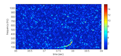
X-Pipeline typically processes data in 256 s blocks. First, it loads the requested data. It constructs a zero-phase linear predictor error filter to whiten the data and estimate the power spectrum Chatterji et al. (2006, 2004). For each sky position, X-Pipeline time-shifts the data from each detector according to equations (1) and (2). The data is divided into overlapping segments and Fourier transformed, producing time-frequency maps for each detector. Given the time-frequency maps for the individual detector data streams $\boldsymbol{\tilde{d}}$, X-Pipeline coherently sums and squares these maps in each pixel to produce time-frequency maps of the desired coherent energies; see Figure 2. This representation gives easy access to the temporal evolution of the spectral properties of the signal, and all statistics and other quantities that are functions of time and frequency.

Figure 2: A simulated $1.4M_{\odot}-10.0M_{\odot}$ neutron star black hole inspiral at an effective distance of 37 Mpc, added to simulated noise from the two LIGO-Hanford detectors. (top) Time-frequency map of the ${E_{+}}$ energy. (bottom) The highest 1% of pixels highlighted. The inspiral “chirp” is clearly visible.

III.3 Clustering and Event Identification

Given time-frequency maps of each of the coherent energies, the challenge is then to identify potential gravitational-wave signals in these maps.

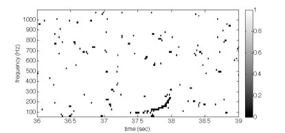
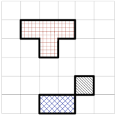
The approach used in X-Pipeline is pixel clustering Sylvestre (2002). The user singles out one of the energy measures – typically ${E_{\mathrm{SL}}}$, the summed energy in the reconstructed ${h_{+}}$ and ${h_{\times}}$ streams – as the detection statistic. A threshold is applied to the detection statistic map so that a fixed percentage (e.g., $1\%$) of the pixels with the highest value in the current map are marked as black pixels; see Figure 2. Following the method of Sylvestre (2002), black pixels that share a common side (nearest neighbors) are grouped together into clusters; see Figure 3 for an example. (As allowed in Sylvestre (2002), the user may specify a different connectivity criterion, such as next-nearest neighbors, or apply the “generalized clustering” procedure.) This clustering technique is appropriate for a GWB whose shape in the time-frequency plane is connected, as opposed to consisting of well-separated “blobs”. This assumption is valid for many well-modeled signals such as low-mass inspirals and ringdowns.

Figure 3: A time frequency map with “black” pixels grouped into 3 clusters. Nearest-neighbor black pixels (those that share an edge) are grouped into a single cluster. Each cluster in this image is denoted by a different color and hatching pattern.

Each cluster is considered a candidate detection event. Each is assigned a detection statistic value from its constituent pixels by simply summing the values of the statistic in the pixels. This is motivated by the additive property of the log-likelihood ratio – the inherited detection statistic is exactly the detection statistic for the area defined by the cluster. Each cluster is also assigned an approximate statistical significance ${\cal S}$ based on the $\chi^{2}$ distribution; see equation (37). This significance is used when comparing different clusters to determine which is the “loudest” – the best candidate for being a gravitational wave signal. Finally, the energy at the same time-frequency locations in maps of each of the other requested likelihoods is also computed and recorded for each cluster.

The clusters are saved for later post-processing. The analysis of time shifting (see equation (2)), FFTing, and cluster identification is then repeated for each of the other sky positions and for each of the requested FFT lengths.

One other important feature of the time-frequency maps is the Fourier transform length or analysis time $T$, which determines the aspect ratio of the pixels. A longer time gives pixels with poor time resolution but good frequency resolution; a shorter time gives pixels with good time resolution but poor frequency resolution. Depending on the signal duration, different analysis times may be optimal. Since each pixel has the same noise distribution (assuming Gaussian statistics), the optimal pixel size is the size for which the signal spans the smallest number of pixels, so that the statistic is least polluted by noise.

Since the optimal analysis time for the incoming signal is not known, X-Pipeline uses several analysis times, and applies a second layer of clustering between analysis times. For this second layer of clustering, clusters made from black pixels at two different analysis times that overlap in time and frequency are compared. The cluster that has the largest significance is kept as a candidate event; the less significant overlapping clusters are discarded.

III.4 Glitch rejection

As noted in Section II, noise glitches tend to have a strong correlation between each coherent energy ${E_{\mathrm{null}}}$, ${E_{+}}$, ${E_{\times}}$, and its corresponding incoherent energy ${I_{\mathrm{null}}}$, ${I_{+}}$, ${I_{\times}}$. X-Pipeline compares the coherent and incoherent energies to veto events that have properties similar to the noise background. These coherent veto tests are applied in post-processing (i.e., after candidate events from the different analysis times are generated and combined).

Two types of coherent veto are available in X-Pipeline. Both are pass/fail tests. The simplest is a threshold on the ratio $I/E$. Following the discussion in Section II.6, a cluster passes the coherent test if

$${I_{\mathrm{null}}}/{E_{\mathrm{null}}} \geq r_{\mathrm{null}}\,,$$ (56)

$$|\log_{10}({I_{+}}/{E_{+}})| \geq \log_{10}(r_{+})\,,$$ (57)

$$|\log_{10}({I_{\times}}/{E_{\times}})| \geq \log_{10}(r_{\times})\,,$$ (58)

where the thresholds $r_{\mathrm{null}}$, $r_{+}$, and $r_{\times}$ may be specified by the user or chosen automatically by X-Pipeline. The form of equations (57) and (58) make these tests two-sided; i.e., they pass clusters that are sufficiently far above or below the diagonal.

Figure 4: ${I_{\mathrm{null}}}$ vs. ${E_{\mathrm{null}}}$ for clusters produced by background noise ($+$) and by simulated gravitational-wave signals ($\Box$). The color axis is the base-10 logarithm of the cluster significance ${\cal S}$. Loud glitches are vetoed by discarding all clusters that fall below the dashed line.

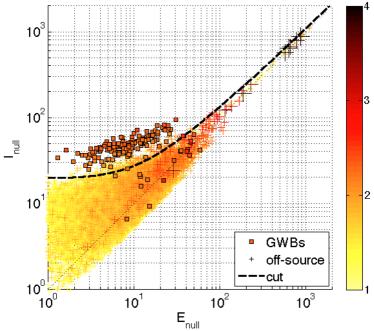
The second type of coherent veto test in X-Pipeline is called the median-tracking veto test. In this test, the exclusion curve is nonlinear and designed to approximately follow the measured distribution of background clusters.

Examination of scatter plots of $I$ vs. $E$ for background clusters shows that, while $I\simeq E$ for loud glitches, there is a bias to $I>E$ at low amplitudes. Furthermore, the width of the distribution of background events around the diagonal varies with $E$. A simple scaling argument shows that for large-amplitude uncorrelated glitches we expect

$$\langle(E-I)^{2}\rangle\propto I\,,$$ (59)

Specifically, for a large single-detector glitch $\tilde{g}(f)$, the correlation with the noise $\tilde{n}(f)$ in another detector will have mean zero and variance $\propto|\tilde{g}|^{2}\propto I$. Consequently, we expect noise events to be scattered about the diagonal with a width that is proportional to $I^{1/2}$ (recall that the energies are dimensionless quantities). The median-tracking test uses this information by estimating the median value of $I$ as a function of $E$ for background events. For each cluster to be tested, it computes the following simple measure $n_{\sigma}$ of how far the cluster is above or below the median:

$$n_{\sigma}\equiv\frac{I-I_{\mathrm{med}}(E)}{I^{1/2}}\,.$$ (60)

An event is passed if

$$n_{\mathrm{null}} > r_{\mathrm{null}}$$ (61)

$$|n_{+}| > r_{+}$$ (62)

$$|n_{\times}| > r_{\times}\,.$$ (63)

As in the ratio test, the thresholds for each energy type are independent and may be specified by the user or selected automatically by X-Pipeline.

The median function $I_{\mathrm{med}}(E)$ is estimated as follows. First, a set of background clusters are binned in $\log_{10}E$ and the median values of $\log_{10}E$ and $\log_{10}I$ in each bin are measured. A quadratic curve of the form

$$\log_{10}I=a(\log_{10}E)^{2}+c$$ (64)

is fit to these sampled medians. The quadratic is merged smoothly to the diagonal $I=E$ above some value of $E$. This shape is entirely ad hoc, but in practice it provides a good fit the observed distribution of glitches.

An example of the median-tracking coherent glitch veto is shown in Figure 4. Each plus symbol ($+$) denotes a background cluster, colored by its significance $\log_{10}{\cal S}$. The large mass of light points at lower left are weak background noise events. The darkly colored points extending along the diagonal to upper right are strong background noise events. Also shown are clusters due to a series of simulated gravitational-wave signals added to the data, denoted by squares ($\Box$). Even though many of these simulated signals are weaker (lighter) than the strong background noise glitches, they are well separated from the background noise population in the two-dimensional $({E_{\mathrm{null}}},{I_{\mathrm{null}}})$ space. The dashed line shows the coherent veto threshold placed on $({E_{\mathrm{null}}},{I_{\mathrm{null}}})$; points below this line are discarded. Scatterplots of ${I_{+}}$ vs. ${E_{+}}$ and ${I_{\times}}$ vs. ${E_{\times}}$ have similar appearance; see Section IV for examples.

In addition to the coherent glitch vetoes, clusters may also be rejected because they overlap data quality vetoes. These are periods when one or more detectors showed evidence of being disturbed by non-gravitational effects that are known to produce noise glitches. Such sources include environmental noise and instabilities in the detector control systems. These data quality vetoes are defined by studies of the data independently of X-Pipeline, and hence are outside of the scope of this report. See Blackburn et al. (2008); Leroy (2009) for recent reviews of data quality and detector characterisation efforts in the LIGO Scientific Collaboration and the Virgo Collaboration.

III.5 Triggered search: tuning and upper limits

We now focus on the strategy for conducting triggered searches with X-Pipeline, specifically searches for gravitational waves associated with gamma-ray bursts (GRBs). As pointed out by Hayama et al. Hayama et al. (2007), GRB searches are an excellent case for the application of coherent analysis, since the sky position of the source is known a priori to high accuracy. We can therefore take full advantage of coherent combinations of the data streams without the false-alarm or computational penalties of scanning over thousands of trial sky directions.

III.5.1 Detection Procedure

For the purposes of a search for unmodelled gravitational-wave emission, a GRB source is characterised by its sky position $\hat{\Omega}$, the time of onset of gamma-ray emission (the trigger time) $t_{0}$, and by the range of possible time delays $\Delta t$ between the gamma-ray emission and the associated gravitational-wave emission. The latter quantity is referred to as the on-source window for the GRB; this is the time interval which is analysed for candidate signals. LIGO searches for gravitational wave bursts associated with GRBs Abbott et al. (2005, 2008a, 2008b) have traditionally used an asymmetric on-source window of $[t_{0}-120\,\textrm{s},t_{0}+60\,\textrm{s}]$, which is conservative enough to encompass most theoretical models of gravitational-wave emission for this source, as well as uncertainties associated with $t_{0}$ Mészáros (2006); Abbott et al. (2005).

In order to claim a detection of a gravitational wave, we need to be able to establish with high confidence that a candidate event is statistically inconsistent with the noise background. In X-Pipeline GRB searches, we use the loudest event statistic Brady et al. (2004); Biswas et al. (2009) to characterise the outcome of the experiment. The loudest event is the cluster in the on-source interval that has the largest significance (after application of vetoes); let us denote its significance by ${\cal S}_{\mathrm{max}}^{\mathrm{on}}$. We compare ${\cal S}_{\mathrm{max}}^{\mathrm{on}}$ to the cumulative distribution $C({\cal S}_{\mathrm{max}})$ of loudest significances measured using background noise (discussed below). We set a threshold on $C({\cal S}_{\mathrm{max}})$ such that the probability of background noise producing a cluster in the on-source interval with significance above this threshold is a specific small value (for example, a 1% chance). The on-source data is then analysed. If the significance $C({\cal S}_{\mathrm{max}}^{\mathrm{on}})$ of the loudest cluster is greater than our threshold, we consider the cluster as a possible gravitational wave detection. We can also set an upper limit on the strength of gravitational-wave emission associated with the GRB in question.

In principle, the cumulative distribution $C({\cal S}_{\mathrm{max}})$ of loudest-event significances for clusters produced by Gaussian background noise can be estimated a priori. In practice, however, real detector data is non-Gaussian. The most straightforward procedure for estimating the background distribution is then simply to analyse additional data from times near the GRB, but outside the on-source interval. These data are referred to as off source. The off-source clusters will not contain a gravitational-wave signal associated with the GRB, and so they can be treated as samples of the noise background. In X-Pipeline, we divide the off-source data into segments of the same length as that used for the on-source data, and analyse each segment in exactly the same manner as the on-source data (using, for example, the same source direction relative to the detectors for computing coherent combinations). For each segment, we determine the significance of the loudest event after applying vetoes. This collection of loudest-event significances from the off-source data then serves as the empirical measurement of $C({\cal S}_{\mathrm{max}})$.

In X-Pipeline we typically set the off-source data to be all data within $\pm 1.5$ hours of the GRB time, excluding the on-source interval. This time range is limited enough so that the detectors should be in a similar state of operation as during the GRB on-source interval, but long enough to provide typically $\sim$50 off-source segments for sampling $C({\cal S}_{\mathrm{max}})$, thereby allowing estimation of probabilities as low as $\sim$2%. To get still better estimates of the background distribution, we also analyse off-source data after artificially time-shifting the data from one or more detectors by different amounts ranging from a few seconds to several hundred seconds. These shifts can give up to approximately 1000 times the on-source data for background estimation, allowing estimation of probabilities at the sub-1% level.

Networks containing both the LIGO-Hanford detectors, H1 and H2, present a special case for background estimation, as local environmental disturbances can produce simultaneous background glitches which are not accounted for in time slides. We therefore do not time-shift H1 relative to H2 unless they are the only detectors operating. In that case, the local probability is computed both with and without time slides to allow a consistency check on the background estimation. (Triggered searches with second-scale on-source windows have the advantage of not requiring time shifts at all; see for example Abbott et al. (2008c).) In practice, we do not see significant differences due to correlated environmental disturbances. We attribute this robustness to the coherent glitch rejection tests described in Section III.4.

III.5.2 Upper Limits

The comparison of the largest significance measured in the on-source data, ${\cal S}_{\mathrm{max}}^{\mathrm{on}}$, to the cumulative distribution $C({\cal S}_{\mathrm{max}})$ estimated from the off-source data allows us to determine if there is a statistically significant transient associated with the GRB. If no statistically significant signal is present, we set a frequentist upper limit on the strength of gravitational waves associated with the GRB. For a given gravitational-wave signal model, we define the 90% confidence level upper limit on the signal amplitude as the minimum amplitude for which there is a 90% or greater chance that such a signal, if present in the on-source region, would have produced a cluster with significance larger than the largest value ${\cal S}_{\mathrm{max}}^{\mathrm{on}}$ actually measured.

We adopt the measure of signal amplitude that is standard for LIGO burst searches, the root-sum-squared amplitude $h_{\mathrm{rss}}$, defined by

$$h_{\mathrm{rss}} = \sqrt{\int_{-\infty}^{\infty}\!\!dt\left[h_{+}^{2}(t)+h_{\times}^{2}(t)\right]},$$ (65)

$$= \sqrt{2\int_{0}^{\infty}\!\!df\left[\tilde{h}_{+}^{2}(f)+\tilde{h}_{\times}^{2}(f)\right]}\,.$$

The units of $h_{rss}$ are Hz^-1/2, the same as for amplitude spectra, making it a convenient quantity for comparing to detector noise curves. For narrow-band signals, the $h_{\mathrm{rss}}$ can also be linked to the energy emitted in gravitational waves under the assumption of isotropic radiation via Riles (2004)

$$E^{\mathrm{iso}}_{\mathrm{GW}}\simeq\frac{\pi^{2}c^{3}}{G}D^{2}f_{0}^{2}h_{\mathrm{rss}}^{2}\,,$$ (66)

where $D$ is the distance to the source and $f_{0}$ is the dominant frequency of the radiation. One drawback of $h_{\mathrm{rss}}$ is that it does not involve the detector sensitivity (either antenna response or noise spectrum). As a result, upper limits phrased in terms of $h_{\mathrm{rss}}$ will depend on the family and frequency of waveforms used, and also on the sky position of the source.

To set the upper limit, we need to determine how strong a real gravitational-wave signal needs to be in order to appear with a given significance. We do this using a third set of clusters, one which contains sample gravitational-wave signals. Specifically, we repeatedly re-analyse the on-source data after adding (“injecting”) simulated gravitational-wave signals to the data from each detector. The data is then analysed as before, producing lists of clusters. The significance associated with a given injection is the largest significance of all clusters that were observed within a short time window (typically 0.1s) of the injection time, after applying vetoes.

The procedure for setting an upper limit is:

1. Select one or more families of waveforms for which the upper limit will be set. For example, a common choice in LIGO is linearly polarized, Gaussian-modulated sinusoids (“sine-Gaussians”) with fixed central frequency and quality factor, and random peak time and polarization angle.

2. Find the significance ${\cal S}_{\mathrm{max}}^{\mathrm{on}}$ of the loudest event in the on-source data, after applying the coherent glitch veto (Section III.4) and any data-quality vetoes.

3. For each waveform family:

   1. Generate random parameter values for a large number of waveforms from the family (e.g., specific peak times and polarization angles for the sine-Gaussian case), and with fixed $h_{\mathrm{rss}}$ amplitude.

   2. Add the waveforms one-by-one to the on-source data, and determine the largest significance of any surviving cluster (after vetoes) associated with each injection.

   3. Compute the percentage of the injections that have ${\cal S}\geq{\cal S}_{\mathrm{max}}^{\mathrm{on}}$.

   4. Repeat 3a–3c using the same waveform family but with different $h_{\mathrm{rss}}$ amplitudes. The 90% confidence-level upper limit is that $h_{\mathrm{rss}}$ for which 90% of the injections have ${\cal S}\geq{\cal S}_{\mathrm{max}}^{\mathrm{on}}$.

III.5.3 Tuning and Closed-Box Analyses

The sensitivity of the pipeline is determined by the relative significance of the clusters produced by real gravitational-wave signals to those produced by background noise. This in turn depends on the details of how the analysis is carried out. In particular, the thresholds used for the coherent glitch rejection tests will have a significant impact on the sensitivity. Too low a threshold will allow background noise glitches to survive, and possibly appear louder than a real gravitational-wave signal. Too high a threshold may reject the gravitational-wave signals we seek.

To improve the sensitivity of X-Pipeline searches, we tune the coherent glitch test to optimize the trade-off between glitch rejection and signal acceptance. We do this using a closed-box analysis. A closed-box analysis estimates the pipeline sensitivity using the off-source and injection data, but not the on-source data. This blind tuning avoids the possibility of biasing the upper limit.

The procedure used for a closed-box analysis follows that used for computing an upper limit, except that an off-source segment is used as a substitute for the true on-source segment. We then test different thresholds for the coherent veto tests, and select the threshold set that gives us the best average “upper limit” estimated from the off-source segments. Specifically, we do the following:

1. For each coherent veto test (${E_{+}}$ vs. ${I_{+}}$, ${E_{\times}}$ vs. ${I_{\times}}$, ${E_{\mathrm{null}}}$ vs. ${I_{\mathrm{null}}}$) we select a discrete set of trial veto thresholds to test.

2. The off-source segments and the injection clusters are divided randomly into two equal sets: one for tuning, and one for upper-limit estimation.

3. For each distinct combination of trial thresholds $(r_{+},r_{\times},r_{\mathrm{null}})$, we do the following:

   1. We apply the coherent veto test (and any data quality vetoes) to the background clusters from each of the tuning off-source segments. The collection of loudest surviving events from each segment gives us $C({\cal S}_{\mathrm{max}})$ for that set of trial thresholds.

   2. We determine the off-source segment that gives the loudest event closest to the $95^{\mathrm{th}}$ percentile of the off-source ${\cal S}_{\mathrm{max}}$ (i.e., closest to $C({\cal S}_{\mathrm{max}})=0.95$). This off-source segment is termed the dummy on-source segment. (Different background segments may serve as the dummy on-source for different trial values of the coherent veto thresholds.)

   3. The dummy on-source clusters and the tuning injection clusters are read, and the coherent vetoes and data-quality vetoes are applied to each. The upper limit is computed, treating the dummy clusters as the true on-source clusters.

4. The final, tuned veto thresholds are the ones that give the lowest upper limit based on the dummy on-source clusters. (If testing multiple waveform families, the upper limits may be averaged across families for deciding the optimal tuning.)

5. To get an unbiased estimate of the expected upper limit, we apply the tuned vetoes to the second set of off-source and injection clusters, that were not used for tuning. Steps 3a – 3c are repeated using the final thresholds, and using the $50^{\mathrm{th}}$ percentile of ${\cal S}_{\mathrm{max}}$ to choose the dummy on-source segment. The upper limit estimated from the dummy on-source segment in this second data set is the predicted upper limit for the GRB; equivalently, it may be interpreted as the sensitivity of the search.

We choose the $95^{\mathrm{th}}$ percentile of ${\cal S}_{\mathrm{max}}$ for tuning to focus on eliminating the tail of high-significance background glitches. This is a deliberate choice, since to be accepted as a detection, a GWB will need to stand well clear of the background. We choose the $50^{\mathrm{th}}$ percentile of ${\cal S}_{\mathrm{max}}$ as the dummy on-source value for sensitivity estimation because this is our best prediction for the typical value of ${\cal S}_{\mathrm{max}}$ in the on-source data under the null hypothesis. Separate data sets are used in tuning and sensitivity estimation to avoid bias from tuning the cuts on the same data used to estimate the sensitivity. The data set used for closed-box sensitivity estimates is later re-used for computing event probabilities and upper limits for the “open-box” (true on-source) data; this introduces no bias because no tuning decisions are made based on the closed-box sensitivity estimate.

In X-Pipeline, the tuning and upper limit calculations are automated. The closed-box analysis is performed first using a pre-selected range of trial thresholds for the coherent glitch test. A web page is generated automatically reporting the details of the closed box analysis, including the optimized threshold values and the predicted upper limits. For the S5/VSR1 search, the user re-runs the post-processing on the on-source data with the fixed optimized thresholds, and another web page report is generated listing detection candidates and upper limits. For the S6/VSR2 search, we propose to automate this “box opening” as well, so that the on-source events are scanned for candidate GWBs immediately once the closed-box tuning analysis has finished.

III.5.4 Statistical and Systematic Errors

There are several sources of error that can affect our analysis. The principal ones are calibration uncertainties (amplitude and phase response of the detectors, and relative timing errors), and uncertainty in the sky position of the GRB.

X-Pipeline is able to account for these effects automatically in tuning and upper limit estimation. Specifically, X-Pipeline’s built-in simulation engine for injecting GWB signals is able to perturb the amplitude, phase, and time delays for each injection in each detector. The perturbations are drawn from Gaussian distributions with mean and variance matching the calibration uncertainties for each detector. Furthermore, the GRB sky position can be perturbed in a random direction by a Gaussian-distributed angle with standard deviation set to the GRB error box width reported by the GCN. Tuning and upper limits based on the perturbed injections are effectively marginalized over these sources of error.

For the S5-VSR1 GRB search, the capability for perturbed injections was not available at the time of the original data analysis, and so the impact of the errors was estimated by re-analysis of a small subset of the full GRB sample. For the S6-VSR2 search, we include calibration and sky-position uncertainties in simulations for all GRBs from the beginning, removing the need to do any additional error analysis.

IV GRB 031108

GRB 031108 Hurley et al. was a long GRB observed by Ulysses, Konus-Wind, Mars Odyssey-HEND and GRS, and RHESSI. As observed by Ulysses, it had a duration of approximately 22 seconds, a 25-100 keV fluence of approximately $2.5\times 10^{-5}$ erg/cm², and a peak flux of approximately $1.8\times 10^{-6}$ erg/cm² s over 0.50 seconds. It was triangulated to a 3-sigma error box with approximate area 1600 square arcminutes with center coordinates 4h 26m 54.86s, $-5^{\circ}\,55^{\prime}\,49.00^{\prime\prime}$.

GRB 031108 occurred during the third science run of the LIGO Scientific Collaboration (“S3”). At that time, the two LIGO-Hanford detectors H1 and H2 were operating, while the Livingston detector L1 was not. A search for gravitational waves associated with the GRB was performed using a cross-correlation algorithm, and reported in Abbott et al. Abbott et al. (2008b).

To demonstrate X-Pipeline, we perform a closed-box analysis of the LIGO H1-H2 data to search for gravitational waves associated with GRB 031108. We tune the search and estimate its sensitivity to gravitational-wave emission as discussed in Section III.5, using the same simulated waveforms as in Abbott et al.. We compare the sensitivity results to those of the cross-correlation search in Abbott et al. We estimate the 90% confidence upper limits from X-Pipeline to be typically 40% lower than those from the cross-correlation search.

IV.1 Analysis

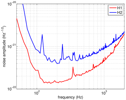
At the time of GRB 031108, the two LIGO Hanford detector H1 and H2 were operating. Figure 5 shows the noise level in the detectors at that time.

Figure 5: Noise spectra of the H1 and H2 detectors at the time of GRB 031108 as estimated by X-Pipeline.

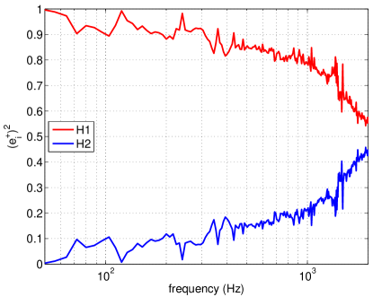
Since the H1 and H2 detectors have identical antenna responses, the network is sensitive to only one of the two gravitational-wave polarizations from any given sky direction. In the DPF, this means that $\boldsymbol{f}{}^{\times}=0$. As a consequence, the cross energy also vanishes identically, ${E_{\times}}=0$, and ${E_{\mathrm{SL}}}={E_{+}}$. Each event cluster is therefore characterised by the two coherent energies ${E_{+}}$ and ${E_{\mathrm{null}}}$, and their associated incoherent components ${I_{+}}$ and ${I_{\mathrm{null}}}$. Figure 6 shows the weighting factors $\boldsymbol{e}{}^{+}$ as a function of frequency.

Figure 6: Normalized contributions to $\boldsymbol{e}{}^{+}\equiv\boldsymbol{f}{}^{+}/|\boldsymbol{f}{}^{+}|$ (in the DPF). Both detectors have the same antenna response, so the coherent weighting at each frequency is determined entirely by the relative noise spectra. Because $\boldsymbol{f}{}^{\times}=0$ for this network, the normalized contribution of detector $i$ to the null stream is simply $1-(e_{i}^{+})^{2}$; i.e., identical to this figure with the H1 and H2 curves swapped.

X-Pipeline was run on all data within $\pm 1$hr of the GRB time for background estimation. Clusters were generated using Fourier transform lengths of 1/8s, 1/16s, 1/32s, 1/64s, 1/128s, and 1/256s. Figure 7 shows scatter plots of ${I_{+}}$ vs. ${E_{+}}$ and ${I_{\mathrm{null}}}$ vs. ${E_{\mathrm{null}}}$ for the half of the off-source clusters that were used for upper limit estimation (i.e., after tuning). Also shown are the clusters produced by simulated sine-Gaussian GWBs at 150 Hz, one of the types tested in Abbott et al. (2008b). These injections had amplitudes of $6.3\times 10^{-21}\mathrm{Hz}^{-1/2}$, approximately equal to the $h_{\mathrm{rss}}$ upper limit estimated from the closed-box analysis.

Figure 7: Scatter plots of off-source ($+$) and simulation ($\Box$) cluster likelihoods: ${I_{+}}$ vs. ${E_{+}}$ (top) and ${I_{\mathrm{null}}}$ vs. ${E_{\mathrm{null}}}$ (bottom). The color denotes $\log_{10}({\cal S})$. Loud background triggers fall close to the diagonal. Simulated gravitational waves also fall close to the diagonal for ${I_{+}}$ vs. ${E_{+}}$, but above the diagonal for ${I_{\mathrm{null}}}$ vs. ${E_{\mathrm{null}}}$. The dashed line denotes the coherent consistency threshold on $({E_{\mathrm{null}}},{I_{\mathrm{null}}})$ that is selected by X-Pipeline’s automated tuning procedure; points below this line are discarded. This test rejects the majority of the loud off-source clusters, while accepting most of the simulated gravitational wave clusters, even if the GWB significiance is typical of background events. The simulated signals in this plot have $h_{\mathrm{rss}}=6.3\times 10^{-21}\mathrm{Hz}^{-1/2}$, approximately equal to the upper limit estimated from the closed-box analysis.

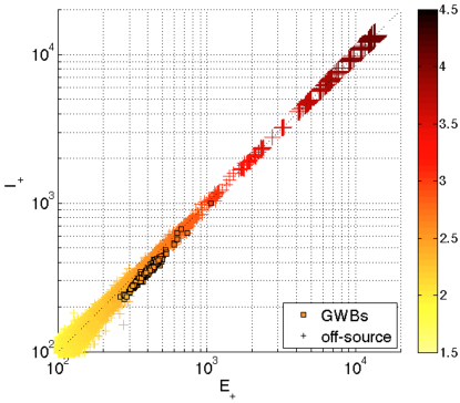
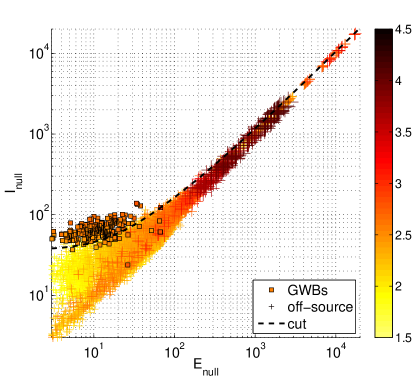
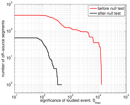
As expected, loud background triggers fall close to the diagonal in both of these plots. The simulated gravitational waves also fall close to the diagonal for ${I_{+}}$ vs. ${E_{+}}$; this is due to the fact that H2 is significantly less sensitive than H1 and so receives very little weighting in the calculation of ${E_{+}}$. In turn, this means that the H1-H2 cross terms in ${E_{+}}$ are small compared to the H1-H1 term, so that ${E_{+}}$ is dominated by the diagonal components and so is very similar to ${I_{+}}$. For the null stream, however, the weightings are reversed, and H2 is weighted higher than H1. As a consequence, gravitational waves lie above the diagonal in the ${I_{\mathrm{null}}}$ vs. ${E_{\mathrm{null}}}$ plot, and it is possible to separate the injections from the background clusters in $({E_{\mathrm{null}}},{I_{\mathrm{null}}})$ space. X-Pipeline’s automated tuning procedure recognizes both of these facts; when run using the median-tracking veto test, it estimates that the best sensitivity will come from requiring a threshold of $r_{+}=5$ on $({E_{\mathrm{null}}},{I_{\mathrm{null}}})$, and imposing no condition on ${I_{+}}$ vs. ${E_{+}}$. The $({E_{\mathrm{null}}},{I_{\mathrm{null}}})$ threshold is indicated in Figure 7 by the dashed line; points below this line are discarded. As can be seen, this test rejects the majority of the loud off-source clusters, while accepting most of the simulated gravitational wave clusters. The off-source clusters that survive the test tend to be of low significance, and therefore will not affect the loudest-event upper limit. Figure 8 shows the distribution of ${\cal S}_{\mathrm{max}}$ before and after the null-stream test.

Figure 8: Distribution of the loudest event significance ${\cal S}_{\mathrm{max}}$ seen in each of the off-source segments used for upper limit estimation, before and after the coherent glitch rejection test. Only 56 of the 391 off-source segments have events that survive the test.

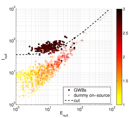
The closed-box analysis discussed in Section III.5 was used to tune the coherent veto test and estimate the expected upper limit from X-Pipeline. Figure 9 shows a scatter plot of the “dummy” on-source clusters. Recall that the dummy on-source region is selected as the background segment that gives the median loudest event surviving the coherent veto test. It therefore represents the expected typical result under the null hypothesis, averaging over noise instantiations, and so is a more robust way to estimate the pipeline sensitivity than, e.g., picking a random segment (or even the on-source segment).

Figure 9: ${I_{\mathrm{null}}}$ vs. ${E_{\mathrm{null}}}$ scatter plot of the dummy on-source ($+$) and simulation ($\Box$) cluster likelihoods used to estimate the upper limit. The color denotes $\log_{10}({\cal S})$. No background events survive the coherent consistency test. The simulated signals in this plot have $h_{\mathrm{rss}}=6.3\times 10^{-21}\mathrm{Hz}^{-1/2}$, approximately equal to the estimated upper limit.

The predicted $h_{\mathrm{rss}}$ upper limits at 90%-confidence for narrow-band sine-Gaussian waveforms of different central frequencies are shown in Table 3 and Figure 10. Table 3 also shows the actual upper limits from the cross-correlation search reported in Abbott et al. (2008b). The predicted X-Pipeline sensitivity is approximately a factor of 1.7 better than that of the cross-correlation pipeline, corresponding to an increase in search volume of a factor of $1.7^{3}\simeq 5$. Similar improvements were seen in the open-box analysis of GRBs in the S5-VSR1 run (2005-2007) Abbott et al. (2010).

frequency (Hz)	100	150	250	554	1000	1850
cross-correlation	18.4	11.3	10.9	12.5	20.4	51.5
X-Pipeline	11.1	6.1	6.5	7.5	12.6	36.7

Table 3: Estimated $h_{\mathrm{rss}}^{90\%}$ amplitude upper limits from X-Pipeline and the best upper limits from the actual cross-correlation search Abbott et al. (2008b). The units are $10^{-21}\mathrm{Hz}^{-1/2}$. The simulated waveforms are circularly polarized sine-Gaussians as described in Abbott et al. (2008b).

Figure 10: 90%-confidence level upper limits on the GW amplitude ($\bullet$) from X-Pipeline for narrow-band circularly polarized sine-Gaussian bursts. The detector noise spectra are also shown for reference.

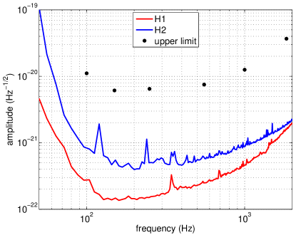
As can been seen in Figure 10, the limiting amplitudes for this GRB track the noise spectrum of H2, and correspond to a matched-filter signal-to-noise ratio of approximately 5 in H2. This occurs because the sensitivity of the analysis is limited by the coherent glitch rejection test. This test requires a measurable correlation between the detectors, which in turn requires that the GWB have some minimal signal-to-noise ratio in each. This behaviour is typical of tuning using the $95^{\mathrm{th}}$ percentile of ${\cal S}_{\mathrm{max}}$, which is an aggressive choice designed to suppress the loud background. While the upper limits tend to be limited by such strong background rejection, our ability to detect a GWB is enhanced, since a GWB candidate will undoubtedly need a significance higher than some very high percentile of the background to be claimed as an actual gravitational wave.

The factor of 1.7 sensitivity improvement of X-Pipeline relative to the cross-correlation search in Abbott et al. (2008b) can be attributed in part to two factors. We estimate that a factor of approximately 1.3 comes from using ${E_{\mathrm{SL}}}$ rather than the cross-correlation as the detection statistic. ${E_{\mathrm{SL}}}$ includes the auto-correlation terms ($\boldsymbol{\tilde{d}}^{\vphantom{*}}_{\mathrm{H1}}\boldsymbol{\tilde{d}}^{*}_{\mathrm{H1}}$, $\boldsymbol{\tilde{d}}^{\vphantom{*}}_{\mathrm{H2}}\boldsymbol{\tilde{d}}^{*}_{\mathrm{H2}}$) in addition to the cross-correlation terms ($\boldsymbol{\tilde{d}}^{\vphantom{*}}_{\mathrm{H1}}\boldsymbol{\tilde{d}}^{*}_{\mathrm{H2}}$) when combining the H1 and H2 data streams. This gives a net increase in the signal-to-noise ratio. More precisely, one can compute the ratio of the expected contribution to ${E_{\mathrm{SL}}}$ due a GWB to the standard deviation in ${E_{\mathrm{SL}}}$ due to Gaussian noise; see Section II.5. Performing the same calculation for the cross-correlation statistic, one finds the per-pixel ratio for ${E_{\mathrm{SL}}}$ to be $1.8\sim 1.3^{2}$ times larger than that for the cross-correlation (assuming a 2:1 ratio in the noise amplitudes for H2:H1). Another factor of $\sim 1.2$ can be attributed to the clustering, which restricts the likelihood calculation to pixels that show significant signal power (and thus tending to exclude pixels that contain only background noise). The cross-correlation statistic in Abbott et al. (2008b) was computed on a minimum time-frequency volume (number of pixels) of approximately 50. By contrast, the typical cluster size in X-Pipeline was found to be 10-30 for injections at the 90% upper limit amplitude. As seen in Section II.5 and Anderson et al. (2001), the amplitude sensitivity in Gaussian noise scales as $N^{-1/4}$. The factor of $\sim 2$ smaller number of pixels used by X-Pipeline should therefore give a factor of $\sim 2^{1/4}=1.2$ sensitivity improvement. Combined with the previous factor of 1.3 gives a total improvement of about 1.6. While this is very close to the average measured improvement, one should keep in mind that these rough estimates have not properly accounted for the non-Gaussianity of the background (which will decrease the sensitivity of both pipelines), or for the tendency of the coherent glitch rejection test to limit the X-Pipeline sensitivity in the absence of strong background glitches. These other effects are presumably also important.

V Autonomous Running

X-Pipeline has been used to process data from S5-VSR1 (2005-2007). This is an “offline” search, being completed almost two years after the last of the GRBs in question was observed. In parallel, X-Pipeline is being improved for the S6-VSR2 run, which started in July 2009. Our goal for S6-VSR2 is fully autonomous running, with a complete analysis of each GRB within 24 hours of the trigger. To achieve this goal requires automatic triggering of X-Pipeline.

V.1 Automated launch of X-Pipeline by GCN triggers

Most of the information for sources which are analyzed by various externally triggered burst searches in LIGO-Virgo come from the GRB Coordinates Network (GCN) gcn . GCN notices and circulars are received in real time by LIGO-Virgo, and the information needed for the search analyses are parsed automatically by perl scripts which are launched each time a GCN notice or circular is received. The information parsed includes: the time and date of the event, the source position (right ascension and declination), the position error, and the duration of the event. For each source, these parameters are compiled and written to a trigger file.

Concurrently, a perl script runs at a central computing site and regularly checks if there are new source events listed in the trigger file. When there are new triggers, the script checks for availability of the LIGO-Virgo data which are necessary for analyzing the source. If the needed data are available, the script launches X-Pipeline event-generation jobs (which include simulation and off-source analyses) on the computing cluster. These jobs are monitored continuously to automatically determine when the jobs have finished. Once they are completed, the post-processing (tuning and detection/upper limit) jobs are automatically launched and likewise monitored. Successful completion of these steps results in a web page in which the results of the analysis are presented, and an email notification being sent to human analysts. Additionally, the scripts which monitor the status of the search and post-processing jobs log that progress for each source event and regularly write this information to a summary status web page. These GCN parsing and triggering scripts are now operational, and X-Pipeline is currently autonomously analysing GRBs from the Swift Gehrels et al. (2004) satellite. Open-box results are available in as little as 6 hours following a GCN alert.

Other modifications currently being made to X-Pipeline focus on the larger sky position error boxes from the Fermi satellite fer . For S6-VSR2, most of the GRB triggers come from the GBM instrument on Fermi, which gives a typical position uncertainty of several degrees. This is much larger than the typical uncertainty of a few arcmin for GRBs from Swift in S5-VSR1. The X-Pipeline launch scripts are currently being modified to set up a grid of sky positions covering this error region, and the handling of events is being modified to minimize the additional computational time required. Finally, the suite of simulated waveforms has been expanded to include binary neutron star and black–hole–neutron–star binary inspirals, since these systems are widely thought to be the progenitors of short GRBs.

VI Summary

X-Pipeline is a software package designed to perform autonomous searches for gravitational-wave bursts associated with astrophysical triggers such as gamma-ray bursts. It performs a fully coherent analysis of data from arbitrary networks of detectors to sensitively search small patches of the sky for gravitational-wave bursts. X-Pipeline features automated tuning of background rejection tests, and a built-in simulation engine with the ability to simulate effects such as calibration uncertainties and sky position errors. X-Pipeline can be launched automatically by receipt of a GCN email, performing a complete analysis of data, including tuning and identification of GWB candidates, without human intervention. Each astrophysical trigger is analysed as a separate search, with background estimation and tuning performed using independent data samples local to the trigger. In a test on actual detector data for a real GRB, we find that X-Pipeline is sensitive to signals approximately a factor of 1.7 weaker than those detectable by the cross-correlation technique used in previous LIGO searches. X-Pipeline has recently been used for the analysis of GRBs from from the LIGO-Virgo S5-VSR1 run, and is currently running autonomously during the S6-VSR2 run to search for gravitational waves associated GRBs observed electromagnetically. Our goal is the rapid identification of possible GWBs on time scales short enough to prompt additional follow-up observations by other observatories.

References

- Ott (2009) C. D. Ott, Classical and Quantum Gravity 26, 063001 (2009), eprint 0809.0695.
- Cutler et al. (1993) C. Cutler, T. A. Apostolatos, L. Bildsten, L. S. Finn, E. E. Flanagan, D. Kennefick, D. M. Markovic, A. Ori, E. Poisson, G. J. Sussman, et al., Phys. Rev. Lett. 70, 2984 (1993).
- Mészáros (2006) P. Mészáros, Rept. Prog. Phys. 69, 2259 (2006), eprint astro-ph/0605208.
- Cutler and Thorne (2002) C. Cutler and K. S. Thorne (2002), eprint gr-qc/0204090.
- Bloom et al. (2009) J. S. Bloom et al. (2009), eprint 0902.1527.
- Kanner et al. (2008) J. Kanner et al., Class. Quant. Grav. 25, 184034 (2008), eprint 0803.0312.
- Van Elewyck et al. (2009) V. Van Elewyck et al., Int. J. Mod. Phys. D18, 1655 (2009), eprint 0906.4957.
- Abbott et al. (2009a) B. P. Abbott et al., Phys. Rev. D 80, 102001 (2009a), eprint 0905.0020.
- Abbott et al. (2009b) B. P. Abbott et al., Phys. Rev. D79, 122001 (2009b), eprint 0901.0302.
- Abbott et al. (2008a) B. Abbott et al., Astrophys. J. 681, 1419 (2008a), eprint 0711.1163.
- Blackburn et al. (2008) L. Blackburn et al., Class. Quant. Grav. 25, 184004 (2008), eprint 0804.0800.
- Leroy (2009) N. Leroy (LIGO Scientific Collaboration and Virgo Collaboration), Class. Quant. Grav. 26, 204007 (2009).
- (13) https://geco.phys.columbia.edu/xpipeline/wiki.
- Chatterji et al. (2006) S. Chatterji, A. Lazzarini, L. Stein, P. Sutton, A. Searle, and M. Tinto, Phys. Rev. D 74, 082005 (2006).
- Abbott et al. (2010) B. P. Abbott et al., The Astrophysical Journal, to appear (2010), eprint 0908.3824.
- Cannon (2008) K. C. Cannon, Classical and Quantum Gravity 25, 105024 (13pp) (2008).
- Anderson et al. (2001) W. G. Anderson, P. R. Brady, J. D. E. Creighton, and E. E. Flanagan, Phys. Rev. D 63, 042003 (2001).
- Sylvestre (2002) J. Sylvestre, Phys. Rev. D 66, 102004 (2002).
- Gursel and Tinto (1989) Y. Gursel and M. Tinto, Phys. Rev. D 40, 3884 (1989).
- Flanagan and Hughes (1998) E. E. Flanagan and S. A. Hughes, Phys. Rev. D 57, 4566 (1998).
- Klimenko et al. (2005) S. Klimenko, S. Mohanty, M. Rakhmanov, and G. Mitselmakher, Phys. Rev. D 72, 122002 (2005).
- Klimenko et al. (2006) S. Klimenko, S. Mohanty, M. Rakhmanov, and G. Mitselmakher, J. Phys. Conf. Ser. 32, 12 (2006).
- Mohanty et al. (2006) S. Mohanty, M. Rakhmanov, S. Klimenko, and G. Mitselmakher, Class. Quant. Grav. 23, 4799 (2006), eprint gr-qc/0601076.
- Rakhmanov (2006) M. Rakhmanov, Class. Quant. Grav. 23, S673 (2006), eprint gr-qc/0604005.
- Klimenko et al. (2008) S. Klimenko, I. Yakushin, A. Mercer, and G. Mitselmakher, Class. Quant. Grav. 25, 114029 (2008), eprint 0802.3232.
- Searle et al. (2008) A. C. Searle, P. J. Sutton, M. Tinto, and G. Woan, Class. Quant. Grav. 25, 114038 (2008), eprint 0712.0196.
- Searle et al. (2009) A. C. Searle, P. J. Sutton, and M. Tinto, Class. Quant. Grav. 26, 155017 (2009), eprint 0809.2809.
- Wen and Schutz (2005) L. Wen and B. Schutz, Class. Quantum Grav. 22, S1321 (2005).
- Hayama et al. (2007) K. Hayama, S. D. Mohanty, M. Rakhmanov, and S. Desai, Class. Quant. Grav. 24, S681 (2007), eprint 0709.0940.
- Tinto (1996) M. Tinto, in Proceedings of the International Conference on Gravitational Waves: Source and Detectors. (World Scientific (Singapore), 1996).
- Sylvestre (2003) J. Sylvestre, Phys. Rev. D 68, 102005 (2003).
- Summerscales et al. (2008) T. Z. Summerscales, A. Burrows, L. S. Finn, and C. D. Ott, The Astrophysical Journal 678, 1142 (2008), eprint 0704.2157.
- Cadonati (2004) L. Cadonati, Class. Quantum Grav. 21, S1695 (2004).
- Fairhurst (2009) S. Fairhurst, New Journal of Physics 11, 123006 (2009).
- Flanagan and Hughes (2005) E. E. Flanagan and S. A. Hughes, New Journal of Physics 7, 204 (2005), eprint gr-qc/0501041.
- Abbott et al. (2004) B. Abbott et al., Nucl. Inst. & Meth. in Phys. Res. 517, 154 (2004).
- Abbott et al. (2009c) B. Abbott et al., Rep. Prog. Phys. 72, 076901 (2009c), eprint arXiv:0711.3041, URL doi:10.1088/0034-4885/72/7/076901.
- Acernese et al. (2008) F. Acernese et al., Classical and Quantum Gravity 25, 114045 (2008).
- Grote et al. (2008) H. Grote et al., Classical and Quantum Gravity 25, 114043 (2008).
- Chatterji et al. (2004) S. Chatterji, L. Blackburn, G. Martin, and E. Katsavounidis, Class. Quant. Grav. 21, S1809 (2004).
- Abbott et al. (2005) B. Abbott et al., Phys. Rev. D 72, 042002 (2005), eprint gr-qc/0501068.
- Abbott et al. (2008b) B. Abbott et al., Phys. Rev. D 77, 062004 (2008b), eprint gr-qc/0709.0766.
- Brady et al. (2004) P. R. Brady, J. D. E. Creighton, and A. G. Wiseman, Class. Quant. Grav. 21, S1775 (2004), eprint gr-qc/0405044.
- Biswas et al. (2009) R. Biswas, P. R. Brady, J. D. E. Creighton, and S. Fairhurst, Classical and Quantum Gravity 26, 175009 (19pp) (2009), eprint 0710.0465.
- Abbott et al. (2008c) B. Abbott et al., Phys. Rev. Lett. 101, 211102 (2008c).
- Riles (2004) K. Riles, LIGO Document: LIGO-T040055-00-Z (2004).
- (47) K. Hurley et al., http://gcn.gsfc.nasa.gov/gcn3/2441.gcn3.
- (48) http://gcn.gsfc.nasa.gov/.
- Gehrels et al. (2004) N. Gehrels, G. Chincarini, P. Giommi, K. O. Mason, J. A. Nousek, A. A. Wells, N. E. White, S. D. Barthelmy, D. N. Burrows, L. R. Cominsky, et al., Astrophys. J. 611, 1005 (2004).
- (50) http://fermi.gsfc.nasa.gov/.