Performance of an externally triggered gravitational-wave burst search

Abstract

We present the performance of searches for gravitational wave bursts associated with external astrophysical triggers as a function of the search sky region. We discuss both the case of Gaussian noise and real noise of gravitational wave detectors for arbitrary detector networks. We demonstrate the ability to reach Gaussian limited sensitivity in real non-Gaussian data, and show the conditions required to attain it. We find that a single sky position search is $\sim$20% more sensitive than an all-sky search of the same data.

I Introduction

Searches for transient gravitational waves (bursts) typically fall into one of two categories: all-sky untriggered searches, which scan the entire sky and search throughout the available data; and triggered or directed searches, which historically analyze only a single point on the sky corresponding to some astrophysical source of interest (see for example Refs. burstS5y2 ; burstGrbS5 ). However, some instruments provide only an approximate sky location for external triggers, which requires scanning a relatively large patch on the sky for an associated gravitational wave. For instance, this is the case for gamma-ray bursts (GRBs) localized by the Gamma-ray Burst Monitor (GBM) Briggs09 ; GBMsysErr_GCN on Fermi, and for some high energy neutrino candidates Baret:2011nu ; 2012arXiv1205.3018T .

We present an implementation of a gravitational wave burst (GWB) search which is able to scan arbitrary sky patches, and demonstrate how the sensitivity of the analysis varies with the sky region searched. In Gaussian noise we find that the sensitivity is a function of the total signal-to-noise-ratio received by the gravitational wave detector network, which is the expected result for an optimal search in Gaussian noise. However for real non-Gaussian gravitational wave detector noise, we find a different dependence of the sensitivity, due to the requirement that the gravitational wave signal be seen by at least two detectors to be distinguished from spurious noise transients. We obtain an empirical formula for the sensitivity of the search in real noise as a function of the sky position for arbitrary detector networks. In particular, a sensitivity loss of $\sim$20% is observed between searching at a single sky position and an all-sky search of the same data.

Finally, we demonstrate the ability to reach Gaussian limited sensitivity in real non-Gaussian data, and show the conditions required to attain it. Specifically, we find that all of the detectors present in the network need to have comparable sensitivity. Moreover, we show that in practice adding a detector to a gravitational wave detector network may actually reduce the search sensitivity for some sky areas when analyzing real data.

We begin in Sec. II with a brief introduction to coherent searches for GWBs. We follow in Sec. III with details of the detection statistic and sky scanning algorithm used in this paper. The spurious-noise rejection tests are presented in Sec. IV. In Sec. V we present the performance of the search for GWBs; in particular, the sky dependence is discussed in Sec. V.1, the comparison between real and Gaussian noise is shown in Sec. V.2, and the dependence on the size of the sky region is presented in Sec. V.3. We conclude with some comments on the implications of these results in Sec. VI.

II Coherent analysis overview

Coherent analysis of gravitational wave data was originally introduced in Ref. Gursel89 . Since then it has proven to be an effective method for GWB searches in LIGO-Virgo data, and it is now the dominant search methodology burstS5y2 ; burstGrbS5 ; S4LIGOGEO ; burstS5y1 ; S5IMBBH ; burstS6allsky ; grb051103 ; grbS6 ; 2012arXiv1205.3018T . Here we give a short overview of coherent analysis in order to introduce notation used in the following sections.

For a gravitational wave $\left(h_{+}(t),h_{\times}(t)\right)$ incoming from a sky location $\hat{\Omega}$ the calibrated data from a gravitational wave detector $\alpha$ are of the form

$$d_{\alpha}(t+\Delta t_{\alpha}(\hat{\Omega}))=\\ F_{\alpha}^{+}(\hat{\Omega})h_{+}(t)+F_{\alpha}^{\times}(\hat{\Omega})h_{\times}(t)+n_{\alpha}(t+\Delta t_{\alpha}(\hat{\Omega}))\,.$$ (1)

Here $F_{\alpha}^{+}(\hat{\Omega})$, $F_{\alpha}^{\times}(\hat{\Omega})$ are the antenna response functions of the given detector to the plus ($+$) and cross ($\times$) polarized gravitational waves, $n_{\alpha}$ is a time series of detector noise, and $\Delta t_{\alpha}(\hat{\Omega})$ is the gravitational wave travel time between the position $\vec{r}_{\alpha}$ of the detector and an arbitrary reference point $\vec{r}_{0}$:

$$\Delta t_{\alpha}(\hat{\Omega})=\frac{1}{c}(\vec{r}_{0}-\vec{r}_{\alpha})\cdot\hat{\Omega}\,.$$ (2)

For the case where the sky location $\hat{\Omega}$ is known a priori, the first step of the analysis is to time shift the data $d_{\alpha}$ by the known $\Delta t_{\alpha}(\hat{\Omega})$ in order to obtain a gravitational wave contribution which is synchronous between the different data time series. The data from each detector are then whitened and decomposed in a time-frequency representation, e.g. using a short Fourier transform or a wavelet decomposition, where the time-frequency basis functions typically have length between several milliseconds and several hundred milliseconds. For a given time-frequency pixel (basis function) of center time $t$ and center frequency $f$ the obtained decomposition can be written compactly as

$$\bm{d}=\bm{F}^{+}h_{+}+\bm{F}^{\times}h_{\times}+\bm{n}\,,$$ (3)

where boldface symbols denote the vector of whitened, time-frequency decomposed time series in the $D$ dimensional space of detectors:

$$\bm{d}=\begin{bmatrix}d_{1}(t,f)/\sqrt{S_{1}(f)}\\ \vdots\\ d_{D}(t,f)/\sqrt{S_{D}(f)}\end{bmatrix}$$ (4a)

$$\bm{n}=\begin{bmatrix}n_{1}(t,f)/\sqrt{S_{1}(f)}\\ \vdots\\ n_{D}(t,f)/\sqrt{S_{D}(f)}\end{bmatrix}$$ (4b)

$$\bm{F}^{+,\times}=\begin{bmatrix}F^{+,\times}_{1}/\sqrt{S_{1}(f)}\\ \vdots\\ F^{+,\times}_{D}/\sqrt{S_{D}(f)}\end{bmatrix}$$ (4c)

Here $S_{i}(f)$ is the one-sided noise power spectrum of detector $i$. Note that the gravitational wave contributions $h_{+}$, $h_{\times}$ are the projection on a time-frequency basis function without any whitening.

The basis used in Eqs. (4) to describe vectors in the $D$ dimensional space of detectors is not adapted to the gravitational wave contribution. Given that the data are whitened and detector noise can be assumed to be uncorrelated between detectors, the vector $\bm{n}$ has an identity covariance matrix, which is invariant under change of orthonormal basis. Hence we can construct a new adapted orthonormal basis, in which the first two vectors span the gravitational wave plane  generated by the $\bm{F}^{+}$ and $\bm{F}^{\times}$ vectors, and the $D-2$ remaining vectors span the null space, the space orthogonal to the gravitational wave plane.

This basis can be further refined in various ways, such as by choosing the first two vectors along the directions of maximal and minimal response to a linearly polarized gravitational wave. These two directions are orthogonal and correspond to the dominant polarization choice Klimenko05 of the arbitrary gravitational wave polarization angle reference, which is a particular choice of the definition of the plus and cross polarizations. We denote the antenna response vectors for this special polarization choice by $\bm{f}^{+}$ and $\bm{f}^{\times}$. They have the properties

$$|\bm{f}^{+}|^{2}\geq|\bm{f}^{\times}|^{2}\,,$$ (5a)

$$\bm{f}^{+}\cdot\bm{f}^{\times}=0\,.$$ (5b)

Note that the choice of which of the plus and cross vector has a larger amplitude is purely conventional. The unit vectors of our adapted basis are hence $\bm{e}^{+}=\bm{f}^{+}/|\bm{f}^{+}|$ and $\bm{e}^{\times}=\bm{f}^{\times}/|\bm{f}^{\times}|$, complemented by vectors spanning the null space, for instance $\bm{e}^{n}=\bm{e}^{+}\wedge\bm{e}^{\times}$ for the case of 3 non-aligned detectors.

An alternative basis choice may be appropriate when we have prior information on the expected gravitational wave polarization. For example, for a circularly polarized gravitational wave signal the projection onto a time-frequency basis function of the two polarizations are related by

$$h_{\times}=\pm ih_{+}\,,$$ (6)

depending on whether the signal is left or right-hand polarized. Hence in the detector space the gravitational wave contribution will lie along either the left or right-handed response vectors

$$\bm{f}^{\circlearrowright}=\bm{f}^{+}+i\bm{f}^{\times},\qquad\bm{f}^{\circlearrowleft}=\bm{f}^{+}-i\bm{f}^{\times}\,,$$ (7)

with corresponding unit vectors $\bm{e}^{\circlearrowright}=\bm{f}^{\circlearrowright}/|\bm{f}^{\circlearrowright}|$, $\bm{e}^{\circlearrowleft}=\bm{f}^{\circlearrowleft}/|\bm{f}^{\circlearrowleft}|$. To construct a left or right-handed basis we use the vectors orthogonal to the response vectors in the gravitational wave plane

$$\bm{f}^{n\circlearrowright}=\frac{\bm{f}^{+}}{|\bm{f}^{+}|^{2}}-i\frac{\bm{f}^{\times}}{|\bm{f}^{\times}|^{2}}\,,\quad\bm{f}^{n\circlearrowleft}=\frac{\bm{f}^{+}}{|\bm{f}^{+}|^{2}}+i\frac{\bm{f}^{\times}}{|\bm{f}^{\times}|^{2}}\,,$$ (8)

with the corresponding unit vectors $\bm{e}^{n\circlearrowright}=\bm{f}^{n\circlearrowright}/|\bm{f}^{n\circlearrowright}|$ and $\bm{e}^{n\circlearrowleft}=\bm{f}^{n\circlearrowleft}/|\bm{f}^{n\circlearrowleft}|$.

Either basis (dominant or circular) can be used to construct two types of statistics: detection statistics and coherent consistency statistics. A detection statistic is used to ranks events as more consistent with a given model of signal buried in noise than a model of noise only. It is usually expressed as the log-likelihood ratio between these two models. Coherent consistency tests, on the other hand, are used to reject spurious noise transients which are usually not included in the noise model of the detection statistic. We discuss the formulation of detection statistics in Sec. III, and coherent consistency tests in Sec. IV; for the moment we note that these statistics are only functions of the data vector $\bm{d}$ and the antenna response vectors $\bm{f}^{+}$ and $\bm{f}^{\times}$ or $\bm{f}^{\circlearrowright},\bm{f}^{\circlearrowleft}$ and $\bm{f}^{n\circlearrowright},\bm{f}^{n\circlearrowleft}$. The value of each statistic is computed independently for each time-frequency pixel, and the resulting values of the detection statistic over the array of time-frequency pixels is used to define gravitational wave events. Specifically, all time-frequency pixels with detection statistic above a certain threshold are clustered to form events, for instance using nearest-neighbor clustering Sylvestre02 . The final detection statistic of such an event is simply the sum of the detection statistic of all the pixels composing the event due to the additive properties of the log-likelihood ratio. The other statistics are also summed over the cluster of pixels composing the event.

This event generation procedure is used on numerous background samples (generated from real data using the time slide technique) and signal samples (generated by adding simulated gravitational wave signals to real data). The obtained background and signal events are used to tune the coherent consistency tests to reject the tail of spurious noise transients inconsistent with the gravitational wave signal hypothesis. Independent samples of background events are then used to estimate the distribution of background events that survive the consistency tests, which is used in turn to define the statistical significance of any candidate gravitational wave events from the analysis of data coincident with the external astrophysical trigger. An independent sample of simulated signal events is used to estimate the sensitivity of the analysis as a function of gravitational wave signal amplitude, and to construct upper limits on the gravitational wave signal amplitude whenever no significant gravitational wave event is found.

III Detection statistic

In a gravitational wave search, the detection statistic is used to ranks events as more consistent with a given model of signal buried in noise than with a model of noise only. The detection statistic is often based on some measure of the energy in the data, motivated by a likelihood-ratio analysis. For the present analysis, we construct a detection statistic following the Bayesian formalism of Ref. Searle08 . The signal model is a circularly polarized gravitational wave signal with Gaussian amplitude distribution of width $\sigma_{h}$, and the noise model is Gaussian. The circular polarization assumption is well motivated for some astrophysical sources, for instance gamma-ray bursts, as discussed in Sec. IV.2. For a right circularly polarized signal we obtain the log-likelihood ratio

$$2L(\bm{d}|\circlearrowright,\sigma_{h})=\frac{|\bm{e}^{\circlearrowright}\cdot\bm{d}|^{2}}{1+1/(\sigma_{h}|\bm{f}^{\circlearrowright}|)^{2}}-\log(1+\sigma_{h}^{2}|\bm{f}^{\circlearrowright}|^{2})\,,$$ (9)

and the left circular polarization log-likelihood ratio $L(\bm{d}|\circlearrowleft,\sigma_{h})$ has an analogous form. The final likelihood ratio is obtained by marginalizing over the left versus right choice, and over a discrete set $\mathcal{A}$ of $\sigma_{h}$ covering the range $[10^{-23},10^{-21}]\,\mathrm{Hz^{1/2}}$ of realistic detectable signals. The detection statistic used thus has the form

$$S_{\text{detection}}=L(\bm{d})=\\ \log\sum_{\sigma_{h}\in\mathcal{A}}\frac{1}{2|\mathcal{A}|}\left[\exp L(\bm{d}|\circlearrowright,\sigma_{h})+\exp L(\bm{d}|\circlearrowleft,\sigma_{h})\right].$$ (10)

The discussion so far has assumed we know the sky position $\hat{\Omega}$ of the gravitational wave source a priori. For some searches this is indeed the case, such as for gamma-ray bursts detected by the Swift satellite BAT05 . In other cases, such as untriggered all-sky searches burstS5y2 ; S4LIGOGEO ; burstS5y1 ; S5IMBBH ; burstS6allsky , $\hat{\Omega}$ is not known, or may only be constrained to some large region of the sky. An example of the latter is gamma-ray bursts detected by the GBM, which has relatively large sky location systematic uncertainties of a few degrees Briggs09 and statistical errors of up to $\sim$10 degrees depending on the $\gamma$-ray flux and spectrum. An error of this size in the sky location used to synchronize the data time series from gravitational wave detectors causes timing discrepancies of up to several milliseconds. A potential gravitational wave signal at a few hundred Hertz could easily be shifted by a quarter of a period or more between a pair of gravitational wave detectors, and the signal could be rejected by a coherent consistency test.

The standard solution in gravitational wave coherent searches is to repeat the analysis over a discrete grid of sky positions covering most of the source sky location probability distribution. Here we use a simple regular grid, composed of concentric circles around the best estimate of the source sky location, which covers at least 95% of the sky location probability distribution. The constant grid step is chosen so that the timing synchronization error between any sky location in the error box and the nearest analysis grid point is less than 10% of the period for the highest frequency gravitational wave signals included in the search. This is small enough to limit the amplitude SNR loss due to timing error to be less than 10%.

Gravitational wave triggers are produced independently for each sky position grid point. The detection statistic $S_{\text{detection}}$, written as a log-likelihood ratio between a signal and a background model, is penalized by the probability $p_{\text{EM}}(\Omega)$ of the trial sky location being the true one, by adding the logarithm of that probability to the detection statistic

$$S_{\text{penalized}}=S_{\text{detection}}+\log p_{\text{EM}}(\Omega)\,.$$ (11)

The reconstructed source sky position for a given signal is the sky position for which the trigger has the largest penalized detection statistic. Only that maximal trigger is kept by the analysis of the grid of sky positions.

As a simple model of $\gamma$-ray satellite errors we use a Fisher probability Briggs99

$$p_{\text{EM}}(\Omega)=p_{\text{Fisher}}(\theta;\kappa)=\frac{\kappa\sin\theta}{\mathrm{e}^{\kappa}-\mathrm{e}^{-\kappa}}\mathrm{e}^{\kappa\cos\theta},$$ (12)

where $\theta$ is the angle between the best estimate sky location and the analyzed one. The parameter $\kappa$ is chosen so that the 95% coverage radius of this Fisher distribution is equal to the 95% coverage radius for a given GRB sky location reconstruction (with statistical and systematic errors added in quadrature). This model is a reasonable approximation for localization performed by a single $\gamma$-ray spacecraft, such as Fermi or Swift, however it may not apply to other instruments, for instance to localization by the Third Interplanetary Network of satellites IPN09 .

IV Coherent consistency tests

IV.1 General framework

Detection statistics such as Eq. (10) are usually constructed assuming the background detector noise is Gaussian. These statistics do not take into account spurious noise transients, mainly because no good model of these transients is available. However these transients are uncorrelated between the different gravitational wave detectors, and powerful coherent consistency tests to reject them can be constructed on that basis Cadonati04 ; Wen05 ; Chatterji06 ; Klimenko08 .

An effective method for rejecting noise transients is to project the gravitational wave data vector $\bm{d}$ onto the null space, and to compare the squared magnitude of this projection with the autocorrelation terms of that projection Chatterji06 . For simplicity let us consider the case of a one dimensional null space along a vector $\bm{e}^{n}$. The squared magnitude of the projection on this vector, also called the coherent null energy, is

$$E_{n}=|\bm{e}^{n}\cdot\bm{d}|^{2}=\sum_{\alpha,\beta}{e^{n*}_{\alpha}}e^{n}_{\beta}\,{d_{\alpha}^{*}}d_{\beta}^{\vphantom{*}}\,.$$ (13)

The autocorrelation part of the null energy, called the incoherent null energy, is

$$I_{n}=\sum_{\alpha}{e^{n*}_{\alpha}}e^{n}_{\alpha}\,{d_{\alpha}^{*}}d_{\alpha}^{\vphantom{*}}=\sum_{\alpha}|e^{n}_{\alpha}|^{2}|d_{\alpha}^{\vphantom{*}}|^{2}\,.$$ (14)

For a strong gravitational wave signal the contribution from the different detectors cancel each other in the coherent null energy, but stay present in the incoherent null energy, hence $E_{n}\ll I_{n}$ is expected. For noise transients the contributions of each detector are expected to be uncorrelated, hence $E_{n}\simeq I_{n}$. Thus, a threshold on the ratio of the incoherent and coherent null energy can be used to reject noise transients.

Several extensions of this framework have been previously implemented and discussed in Ref. Sutton10 . First, the separation between the coherent and incoherent energy for both noise transients and gravitational wave signals depends on the value of the incoherent energy, that is the strength of the deviation from the Gaussian noise hypothesis, hence a more complicated separation line in the coherent/incoherent energy plane than a simple ratio is used in practice. Second, the framework has also been extended to projection vectors that are not in the null space, but in the gravitational wave plane. The incoherent energy will remain comparable to the coherent energy for the case of noise transients, but for gravitational wave signals it will be much smaller or larger than the coherent energy. The previously proposed extension Sutton10 is to use the plus and cross polarization directions in the dominant polarization frame. Along $\bm{e}^{+}$ a coherent buildup of energy is expected for most gravitational wave signals; this projection corresponds to the hard constraint introduced in Ref. Klimenko05 . On the other hand, for many network configurations and large fractions of the sky $|\bm{f}^{\times}|\ll|\bm{f}^{+}|$ Klimenko05 , and the projection on the $\bm{e}^{\times}$ vector can be considered as an effective null stream.

IV.2 Extension to circular polarization

The main issue with the previously described projections is that none of them is effective for the case of two gravitational wave detectors which see roughly independent linear polarizations , which occurs frequently for networks consisting of one LIGO detector plus Virgo. In that case the coherent consistency tests based on the plus and cross energies perform poorly, as the cross-correlation terms are small, and the incoherent and coherent energy are roughly equal for both gravitational waves and noise transients. This issue was noted in the all-sky GWB search of 2005-2007 LIGO-Virgo data burstS5y2 , and can also be seen in the poor upper limits for the search in association with GRBs of the same data burstGrbS5 .

Here we propose to expand the possible projection vectors using the assumption of a circularly polarized gravitational wave signal. This imposes correlations between otherwise independent linear polarizations, and allows us to construct effective consistency tests even for the case of two strongly misaligned gravitational wave detectors. Also, we note that the circular polarization assumption is well motivated for many astrophysical scenarios. For instance, for gamma-ray bursts the expected beamed emission of the gamma rays means that the progenitor is seen roughly along its axis of rotation. Furthermore, gravitational wave emission models which could be seen at extra-galactic distances emit predominantly circularly polarized gravitational waves along their rotation axis Kobayashi03-1 ; Shibata03 ; Davies02 ; Piro07 ; Romero10 .

We consider the projection onto the manifold of circularly polarized gravitational waves, which is formed by the two complex lines along the left and right handed polarization directions. The magnitude of the projection is simply the maximum of the projection on the left and right handed response unit vectors $\bm{e}^{\circlearrowright}$ and $\bm{e}^{\circlearrowleft}$, which we defined in Sec. II,

$$E_{\text{circular}}=\max\left(|\bm{e}^{\circlearrowright}\cdot\bm{d}|^{2},|\bm{e}^{\circlearrowleft}\cdot\bm{d}|^{2}\right)\,.$$ (15)

This projection can be compared to its incoherent part

$$I_{\text{circular}}=I_{\circlearrowright}=I_{\circlearrowleft}\,,$$ (16)

which is equal for the right and left projections. Using the pair of incoherent/coherent energies $E_{\text{circular}},I_{\text{circular}}$ a consistency test can be constructed analogously to the ones based on the plus or cross energies.

Furthermore, given the circular polarization assumption a null test can be constructed by considering the unit vectors $\bm{e}^{n\circlearrowright}$ and $\bm{e}^{n\circlearrowleft}$ that are orthogonal to the circular projection and defined in Sec. II. The null circular energy is defined as the minimum of the magnitude of the projection onto these two unit vectors

$$E_{\text{null circular}}=\min\left(|\bm{e}^{n\circlearrowright}\cdot\bm{d}|^{2},|\bm{e}^{n\circlearrowleft}\cdot\bm{d}|^{2}\right).$$ (17)

As in the previous cases an incoherent counterpart can be defined, with the autocorrelation terms of the null left and right projection being equal. A consistency test can then be constructed using $E_{\text{null circular}}$, $I_{\text{null circular}}$.

V Analysis performance

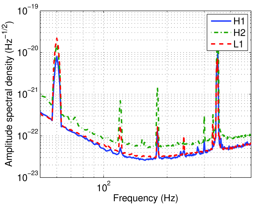
Figure 1: Strain noise spectra from the LIGO detectors used in this study. Note that H2 data are treated as if the detector was located at the Virgo site in order to simulate the gravitational wave detector network operated in 2009-2010.

The analysis methodology described above has been implemented in X-Pipeline Sutton10 , a software package designed for GWB searches in association with external astrophysical triggers. Earlier versions of this package have been used to search for GWBs associated with GRBs burstGrbS5 ; grb051103 .

In order to understand the sky dependence of the sensitivity of GWB searches, we study the performance of X-Pipeline in searching for circularly polarized gravitational wave bursts. Specifically, we characterize the performance for a typical GRB-trigger scenario for the most recent science run of the LIGO-Virgo network iLIGO ; Virgo ; Virgo11 , from 2009-2010. Since data from that period have not yet been released for data analysis performance studies of the type presented here, we use as a proxy a 3 hour long sample of LIGO data from 23 February 2006. At that time the two detectors at the Hanford site and the detector at the Livingston site were taking science quality data; the spectra of the data at the center of that sample are shown on Fig. 1. To be representative of the full network of large scale interferometric gravitational wave detectors which was operational during 2009-2010, we use the data from 2 km detector Hanford site as if that detector was located at the Virgo site, hence throughout this article we will denote these data as from V1. The factor $\sim$2 difference in sensitivity is roughly representative in the difference in sensitivity between Virgo and the two 4 km LIGO detectors (H1 and L1) in the 2009-2010 data set.

These data are used to generate background data samples using the time slide method, and to generate simulated signal samples by adding circularly polarized sine-Gaussian and compact binary inspiral waveforms into these data. We perform full autonomous analyses as used in real externally triggered gravitational wave searches to determine the sensitivity for these signal models. We use a 660 s long time window around fiducial external triggers, and search for gravitational waves over the frequency band 64$-$500 Hz. These are the parameters used in the search for gravitational waves associated with GRBs in 2009-2010 LIGO-Virgo data grbS6 . For reference, we also use simulated Gaussian noise with the same spectral properties. With this reference the effect of non-Gaussian noise transients present in real data can be assessed.

V.1 Single sky position analysis

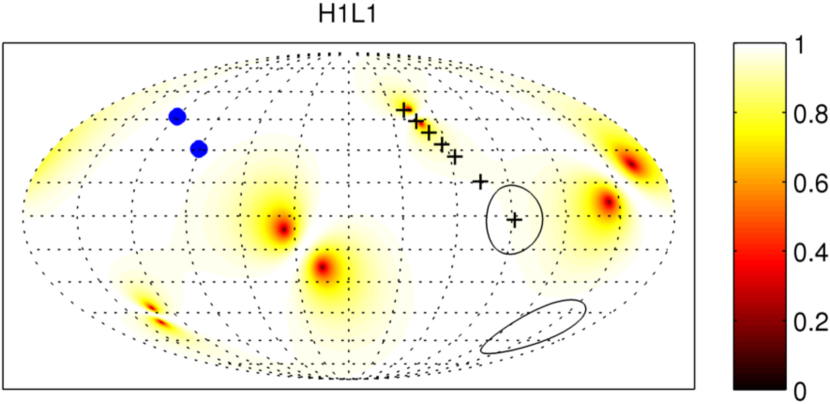
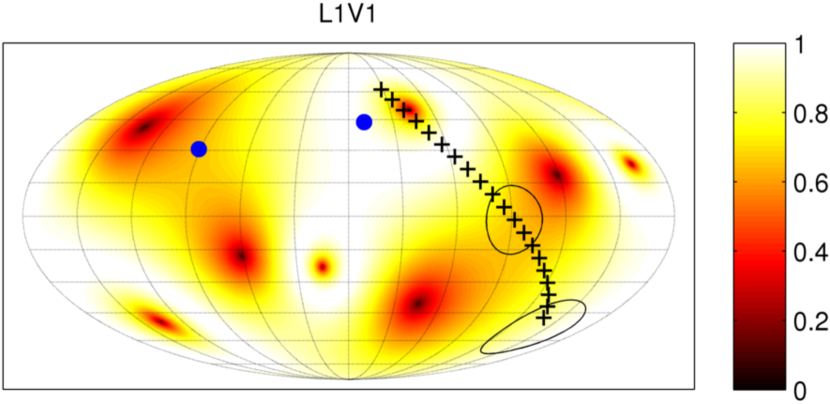
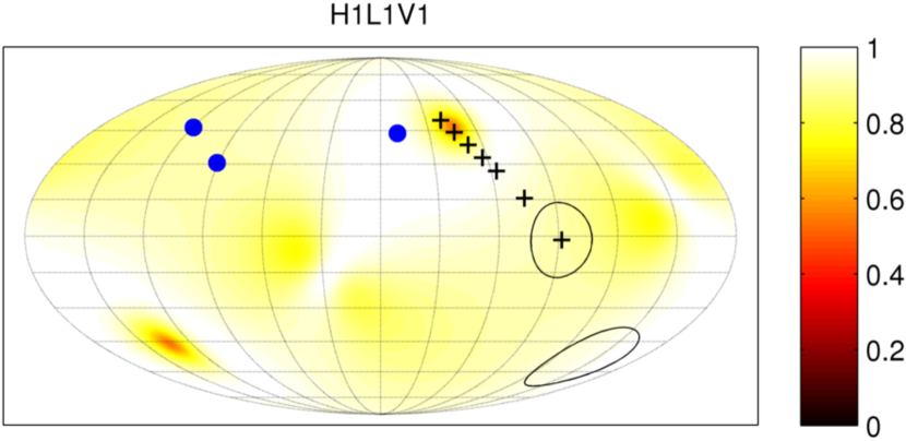
Figure 2: Sky dependence of the penalty factor $\lambda_{c}/\rho_{c}$ [Eq. (22)] assuming that V1 is a factor 2 less sensitive than H1 and L1. From top to bottom the penalty factor for respectively the H1L1, L1V1 and H1L1V1 networks are shown. The coordinates used are the longitude and latitude in a Mollweid projection, as the detectors are fixed to the Earth. The location of the detectors in each network are marked by blue dots; for each detector the projection on the celestial sphere of the location (and its opposite) are the points of maximum antenna response. For the 2 detector networks the zero points of the penalty factor correspond to the null of the antenna response for one of the two detectors. The plus marks show the sky location of the fiducial triggers analyzed to produce Fig. 3, whereas the circles show the large sky regions used for the study shown in Fig. 5. We omit the map for the H1V1 network as it is very similar to the L1V1 map.

To study the effect of different antenna pattern configurations, we perform the analysis of fiducial external triggers well localized to different points in the sky, which is representative of gamma-ray bursts reported by Swift. We use the same time for all these external triggers, but select sky locations which probe different combinations of contributions from the various detectors in the gravitational wave detector network. The fiducial sky locations and gravitational wave detector networks used in this study are shown on the 3 panels of Fig. 2.

In order to have an a priori measure of the signal strength with regard to the detectors noise, we define the coherent network SNR Finn01

$$\rho_{c}=\sqrt{\sum_{\alpha\in\text{network}}\rho_{\alpha}^{2}}$$ (18)

of a gravitational wave signal model as the root-sum-square of the individual SNRs

$$\rho_{\alpha}^{2}=4\int_{0}^{\infty}\frac{|F^{+}_{\alpha}h_{+}(f)+F^{\times}_{\alpha}h_{\times}(f)|^{2}}{S_{\alpha}(f)}\,\mathrm{d}f$$ (19)

of that signal in each detector $\alpha$ across the network. This figure of merit can be used as a predictor of the gravitational wave signal amplitude (distance to the source) needed for the signal to be detected.

We define the detection sensitivity of the search for a particular signal model as the distance $d_{50\%}$ at which that signal is found with $50\%$ efficiency while holding the background false-alarm probability fixed at $1\%$ per on-source window (in this case 1% per 660 s, or a false alarm rate of $1.5\times 10^{-5}$ Hz). This detection sensitivity is estimated by adding gravitational wave signals into either real or simulated detector noise; approximately $10^{4}$ such “injections” are performed spread over 2 decades in distance. We use as our model signal a circularly polarized Gaussian-modulated sinusoid with central frequency $f_{0}=150$ Hz and $Q=9$,

$$\begin{bmatrix}h_{+}(t)\\ h_{\times}(t)\end{bmatrix}=\frac{A}{d}\begin{bmatrix}\cos(2\pi f_{0}t)\\ \sin(2\pi f_{0}t)\end{bmatrix}\exp\left[-\frac{(2\pi f_{0}t)^{2}}{2Q^{2}}\right]\,.$$ (20)

Here $A$ is an arbitrary scaling factor and $d$ the distance to the source. This is a standard waveform for evaluating the sensitivity of triggered GWB searches burstGrbS5 ; grb051103 ; grbS6 ; 2012arXiv1205.3018T ; 2008PhRvD..77f2004A .

For an ideal matched filter search in Gaussian noise $d_{50\%}$ should correspond to the distance at which the median of $\rho_{c}$ for that signal model crosses a certain threshold. This threshold depends on the number of degrees of freedom of the filtering template and the effective number of independent times. For the search considered here, the number of independent trials is of the order of $3\times 10^{5}$: the total time-frequency volume in the on-source window. The false alarm probability per trial is thus approximately $3\times 10^{-8}$. The number of degrees of freedom is 2 (real and imaginary parts of the data) times the number of time-frequency pixels in a Gaussian noise cluster (typically in the 4$-$6 range). Hence using a $\chi^{2}$ distribution for Gaussian noise we obtain an expected threshold on $\rho_{c}$ in the 7.1$-$7.7 range.

However, for an analysis of real data, $\rho_{c}$ is not necessarily a good figure of merit, as a signal needs also to pass coherent consistency tests to be distinguished from non-Gaussian noise transients. Heuristically, a signal needs a sufficient $E-I$ difference that Gaussian noise fluctuations will not destroy the signal consistency as seen by the coherent tests described in Sec. IV. Empirically we find that the penalized coherent SNR

$$\lambda_{c} =\rho_{c}\left[\frac{N_{\text{det}}+1}{N_{\text{det}}-1}\frac{E_{\text{circular}}^{\text{signal}}-I_{\text{circular}}^{\text{signal}}}{E^{\text{signal}}_{\text{circular}}+I_{\text{circular}}^{\text{signal}}}\right]^{1/4}$$ (21)

$$=\rho_{c}\left[\frac{N_{\text{det}}+1}{N_{\text{det}}-1}\frac{\sum_{\alpha\neq\beta}|f_{\alpha}^{\circlearrowright}|^{2}|f_{\beta}^{\circlearrowright}|^{2}}{|\bm{f}^{\circlearrowright}|^{4}+\sum_{\alpha}|f_{\alpha}^{\circlearrowright}|^{4}}\right]^{1/4},$$ (22)

where $N_{\text{det}}$ is the number of detectors in the network, is a good figure of merit for signals in non-Gaussian noise from real gravitational wave detectors . The normalization factor $(N_{\text{det}}+1)/(N_{\text{det}}-1)$ is chosen so that the penalty factor $\lambda_{c}/\rho_{c}$ has a maximum value of 1. Note that the magnitudes of the right and left-handed sensitivity vectors are equal

$$|f_{\alpha}^{\circlearrowright}|=|f_{\alpha}^{\circlearrowleft}|=\left({f_{\alpha}^{+}}^{2}+{f_{\alpha}^{\times}}^{2}\right)^{1/2},$$ (23)

so it does not matter which is used to evaluate Eq. (22).

The distribution on the sky of the penalty factor for different networks is shown in Fig. 2. The maximum of the factor for any network is attained when the sensitivity of all detectors in the network is equal, that is when all $|f_{\alpha}^{\circlearrowright}|$ are equal. For the 2 detector networks the zero points of the penalty factor correspond to the blind spots of one of the two detectors in the network.

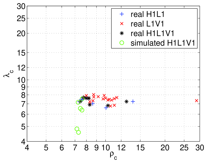
Figure 3: Values of $\rho_{c}$ and $\lambda_{c}$ corresponding to the detection sensitivity $d_{\text{50\%}}$ found when analyzing real and simulated Gaussian noise. Each marker represents a complete end-to-end analysis for one of the networks and sky positions indicated in Fig. 2. Plus marks are for real noise from the H1L1 network, cross marks for real noise from the L1V1 network, star marks for real noise from the H1L1V1 network, and circles are for simulated Gaussian noise from the H1L1V1 network. The analyzed sky position are shown as crosses on Fig. 2.

The test sky positions used in the comparison are also shown in Fig. 2. They are chosen along a line which samples a wide range of penalty factors, in order to distinguish $\lambda_{c}$ and $\rho_{c}$. We use a larger sample of test sky positions for the L1V1 network, as this is the network for which the penalty factor effect is most important.

For each of the trigger sky positions and networks indicated in Fig. 2 we perform a complete analysis using both simulated Gaussian noise and real data. In each case we compute the distance sensitivity $d_{\text{50\%}}$ at which the source model (20) is detectable with 50% probability at a fixed false alarm probability of 1%. The values of $\rho_{c}$ and $\lambda_{c}$ corresponding to this $d_{\text{50\%}}$ are then computed for each test sky position; see Fig. 3. For simulated noise we obtain the expected result that $d_{\text{50\%}}$ corresponds to a threshold on $\rho_{c}$, here equal to $\sim 7.4$, which falls into the expected range of $7.1-7.7$. However, for real noise the obtained value of $\rho_{c}$ is spread over a much larger range of $7.5-30$, whereas $\lambda_{c}$ fluctuates by only 5% around $\sim 7.5$. Two conclusions can be drawn from these results:

1. $\lambda_{c}$ is a good predictor of the analysis sensitivity in real noise as a function of sky position for a given signal model;

2. A sensitivity as good as in Gaussian noise ($\lambda_{c}\sim\rho_{c}$) can be attained for sky positions where the penalty factor is close to 1. This occurs where all detectors have comparable sensitivity, which corresponds to the white areas on Fig. 2.

V.2 Distribution of sensitive distance

The good performance of the penalized coherent SNR $\lambda_{c}$ in predicting the sensitivity of real data analysis allows us to study analytically the sensitivity sky dependence, and to compare it with the Gaussian noise case which is given by $\rho_{c}$.

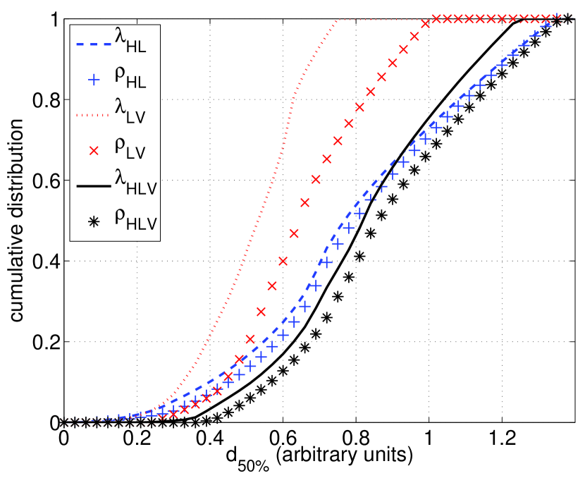
Figure 4: Cumulative distribution over the sky of the sensitive distance $d_{50\%}$ assuming that V1 is a factor 2 less sensitive than H1 and L1. The lines show the distribution when $d_{50\%}$ is assumed to be given by a threshold on $\lambda_{c}$ (real data analysis): blue dashed line for the H1L1 network, red dotted line for the L1V1 network and black solid line for the H1L1V1 network. The marks show the distribution when $d_{50\%}$ is assumed to be given by a threshold on $\rho_{c}$ (Gaussian data analysis): blue pluses for the H1L1 network, red crosses for L1V1 network and black stars for the H1L1V1 network.

Fig. 4 shows the cumulative distribution of the sensitive distance $d_{50\%}$ assuming that V1 is a factor 2 less sensitive than H1 and L1. We consider two cases: a Gaussian noise analysis where the sensitivity is given by a threshold on $\rho_{c}$ and a real noise analysis where the sensitivity is predicted by the same threshold but on $\lambda_{c}$.

For the H1L1 network the real and Gaussian noise sensitivities are very close; our analysis of real data is only a few percent less sensitive than the ideal Gaussian case. However for networks including Virgo, especially for the L1V1 network of two non-aligned detectors, the sensitivity is as much as 20% lower with real data than with ideal Gaussian noise. This is an expected effect of each detector having maximum antenna response near the null response of the other detector, which limits the spurious transient noise rejection methods as they rely on the signal being visible above the Gaussian part of the noise in at least two detectors.

Interestingly for 30% of the sky the sensitivity of the H1L1V1 network is slightly worse than that of the H1L1 network for the real data case. The sensitivity loss occurs for areas of the sky where the antenna patterns are optimal for the H1 and L1 detectors, and relatively poor for V1. Hence for these sky regions Virgo brings additional non-stationary noise but only a very small increase in the total gravitational wave signal. We note that the sensitivity difference is less than 10%, and is a consequence of the non-optimality of our analysis of real data (the optimal procedure for real data is not known). To verify this prediction, we repeat the full end-to-end analysis of a dozen sky positions in those regions for both the H1L1 and H1L1V1 network. The comparison of the obtained $d_{50\%}$ confirms that the H1L1V1 network is less sensitive in those sky regions by up to 10%. This indicates that care should be taken when selecting detectors for the analysis of real data in mis-aligned networks.

V.3 Large sky area analysis

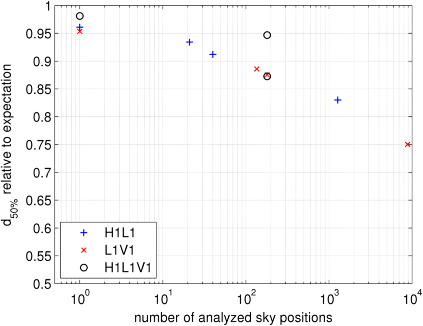
Figure 5: Fractional value of $d_{\text{50\%}}$ for real detector noise as a function of the number of analyzed sky positions relative to the expectation based on the typical threshold $\lambda_{c}=7.5$, which we obtained in Fig. 3. Blue plus marks denote results for the H1L1 network, red cross marks for the L1V1 network and black circle marks for the H1L1V1 network. The 6 marks around 100 sky positions correspond to search sensitivity over the sky patches represented as circles on Fig. 2. The 2 marks with sky position number > 1000 correspond to search sensitivity over the full sky.

In principle, searching over a large sky area should lower the sensitivity, due to the trials factor incurred from repeating the analysis over a grid of sky positions. We have seen that the penalized coherent SNR $\lambda_{c}$ is a good figure of merit for the sensitivity of X-Pipeline as a function of a single sky position. We therefore expect that for large sky areas the 50% efficiency distance $d_{50\%}$ should correspond to a threshold on the median value of $\lambda_{c}$ over the analyzed sky area, where the median takes into account the prior $p_{\text{EM}}(\Omega)$ on the true source sky position. Due to the trials factor, the threshold on this median $\lambda_{c}$ will typically be slightly higher than in the single sky position case, and the ratio between the two yields an estimate of the sensitivity loss due to a large sky area analysis.

To assess this sensitivity loss we repeat the analysis using typical sky location uncertainties for the GBM instrument on Fermi: a $5^{\circ}$ statistical error and two-component systematic error as described in Ref. GBMsysErr_GCN . This results in a search grid of $\sim$700 square degrees in area. Due to limited computational resources only a small number of sky regions and network combinations are used; the analysed sky regions are shown as circles on Fig. 2. For completeness, we also perform a full-sky analysis for the H1L1 and L1V1 networks.

The resulting sensitive distances $d_{\text{50\%}}$ relative to the expected value for a single sky point analysis are shown in Fig. 5. We find that the performance loss of GBM-type error regions compared to precisely-localized external triggers is less than 10%. A complete lack of sky position information (requiring an all-sky search) decreases the sensitivity by $\sim 20\%$. Hence the availability of external triggers which are well localized on the sky ($\lesssim 1\,\mathrm{deg^{2}}$) improves the sensitivity by up to 20%. This is in addition to the sensitivity improvement resulting from the known time of the trigger, which reduces the trials factor from the length of data to be searched Kochanek93 .

VI Conclusion

We have studied how the sensitivity of a search for GWBs performed by X-Pipeline depends on the sky region specified by an external astrophysical trigger. Two aspects of the sky region affect the search sensitivity: the magnitudes of the antenna patterns of the various gravitational wave detectors in the network over this region; and the area of the region, which affects the size of the parameter space of the search.

For the case of Gaussian background noise we have obtained the result expected for an optimal analysis, namely the sensitivity is given by a threshold on the coherent SNR $\rho_{c}$, and this threshold falls into the range predicted by a $\chi^{2}$ distribution given the number of independent trials in the search.

For real data we introduce a penalized coherent SNR $\lambda_{c}$, which proves to be a good predictor of the search sensitivity in real non-Gaussian noise. It is expressed as the coherent SNR times a penalty factor; this penalty factor is equal to 1 (no penalty) if all detectors have equal sensitivity for a given sky position, and to 0 if only one of the detectors is sensitive. For regions of the sky where the penalty factor is equal to 1, the sensitivity in real noise is as good as in the Gaussian noise case.

The penalized coherent SNR $\lambda_{c}$ allows us to separate the effect of antenna patterns changing over the sky from the effect of a search parameter space increase due to a large search sky region. We find that trigger information that allows us to restrict the search to a single sky position increases the sensitivity by $\sim 20\%$ compared to searching over the whole sky, and by $\sim 10\%$ compared to searching over error boxes of a few hundred square degrees. This addresses part of the long-standing question on how externally triggered searches relate to all-sky and all-time searches for gravitational waves.

- (1) J. Abadie et al., Phys. Rev. D 81, 102001 (2010)
- (2) B. P. Abbott et al., Astrophys. J. 715, 1438 (2010)
- (3) M. Briggs et al., AIP Conf. Proc. 1133, 40 (2009)
- (4) V. Connaughton, GCN circular 11574 (2011)
- (5) B. Baret et al., Phys. Rev. D 85, 103004 (2012)
- (6) S. Adrián-Martínez et al.(May 2012), arXiv:1205.3018
- (7) Y. Gürsel and M. Tinto, Phys. Rev. D 40, 3884 (1989)
- (8) B. Abbott et al., Classical and Quantum Gravity 25, 245008 (Dec. 2008)
- (9) B. P. Abbott et al., Phys. Rev. D 80, 102001 (2009)
- (10) J. Abadie et al.(Jan. 2012), arXiv:1201.5999
- (11) J. Abadie et al.(Feb. 2012), arXiv:1202.2788
- (12) J. Abadie et al.(2012), arXiv:1201.4413
- (13) J. Abadie et al.(2012), arXiv:1205.2216
- (14) For simplicity we consider only the case of a network composed of non-aligned detectors, as in the most recent science run of the LIGO-Virgo detector network (only one gravitational wave detector was operational at the LIGO-Hanford site during the 2009-2010 run).
- (15) S. Klimenko, S. Mohanty, M. Rakhmanov, and G. Mitselmakher, Phys. Rev. D 72, 122002 (2005)
- (16) J. Sylvestre, Phys. Rev. D 66, 102004 (2002)
- (17) A. C. Searle, P. J. Sutton, M. Tinto, and G. Woan, Class. Quantum Grav. 25, 114038 (2008)
- (18) S. D. Barthelmy et al., Space Sci. Rev. 120, 143 (2005)
- (19) M. Briggs et al., Astrophys. J. Suppl. Ser. 122, 503 (1999)
- (20) K. Hurley et al., AIP Conf. Proc 1133, 55 (2009)
- (21) L. Cadonati, Class. Quantum Grav. 21, S1695 (2004)
- (22) L. Wen and B. F. Schutz, Class. Quantum Grav. 22, S1321 (2005)
- (23) S. Chatterji et al., Phys. Rev. D 74, 082005 (2006)
- (24) S. Klimenko, I. Yakushin, A. Mercer, and G. Mitselmakher, Class. Quantum Grav. 25, 114029 (2008)
- (25) P. J. Sutton et al., New J. Phys. 12, 053034 (2010)
- (26) This happens when the orientation of the detector arms differs by when projected onto the plane orthogonal to the gravitational wave direction of propagation.
- (27) S. Kobayashi and P. Mészáros, Astrophys. J. Lett. 585, L89 (2003)
- (28) M. Shibata, K. Shigeyuki, and E. Yoshiharu, Mon. Not. R. Astron. Soc. 343, 619 (2003)
- (29) M. B. Davies, A. King, S. Rosswog, and G. Wynn, Astrophys. J. Lett. 579, L63 (2002)
- (30) A. L. Piro and E. Pfahl, Astrophys. J. 658, 1173 (2007)
- (31) G. E. Romero, M. M. Reynoso, and H. R. Christiansen, Astron. Astrophys. 524, A4 (2010)
- (32) B. P. Abbott et al., Rep. Prog. Phys. 72, 076901 (2009)
- (33) T. Accadia et al., JINST 7, P03012 (2012)
- (34) T. Accadia et al., Class. Quantum. Grav. 28, 114002 (2011)
- (35) L. S. Finn, Phys. Rev. D 63, 102001 (2001)
- (36) B. Abbott et al., Phys. Rev. D 77, 062004 (Mar. 2008)
- (37) Equation (22) follows from (21) provided the relative noise levels do not vary significantly across the bandwidth of the signal.
- (38) C. S. Kochanek and T. Piran, Astrophys. J. Lett. 417, 17 (1993)