Gravitational waves from remnant massive neutron stars of binary neutron star merger: Viscous hydrodynamics effects

Abstract

Employing a simplified version of the Israel-Stewart formalism of general-relativistic shear-viscous hydrodynamics, we explore the evolution of a remnant massive neutron star of binary neutron star merger and pay special attention to the resulting gravitational waveforms. We find that for the plausible values of the so-called viscous alpha parameter of the order $10^{-2}$, the degree of the differential rotation in the remnant massive neutron star is significantly reduced in the viscous timescale, $\lesssim 5$ ms. Associated with this, the degree of non-axisymmetric deformation is also reduced quickly, and as a consequence, the amplitude of quasi-periodic gravitational waves emitted also decays in the viscous timescale. Our results indicate that for modeling the evolution of the merger remnants of binary neutron stars, we would have to take into account magnetohydrodynamics effects, which in nature could provide the viscous effects.

I Introduction

The merger of binary neutron stars is one of the promising sources of gravitational waves for ground-based gravitational-wave detectors such as advanced LIGO, advanced VIRGO, and KAGRA detectors . This fact has motivated the community of numerical relativity to construct a reliable model for the inspiral, merger, and post-merger stages of binary neutron stars by numerical-relativity simulations.

The recent discoveries of two-solar mass neutron stars twosolar strongly constrain the possible evolution processes in the merger and post-merger stages, because the presence of these heavy neutron stars implies that the equation of state of neutron stars has to be stiff enough to support the self-gravity of the neutron stars with mass $\gtrsim 2M_{\odot}$. Numerical-relativity simulations with a variety of hypothetical equations of state that can reproduce the two-solar-mass neutron stars have shown that massive neutron stars surrounded by a massive torus are likely to be the canonical remnants formed after the merger of binary neutron stars of typical total mass 2.6–$2.7M_{\odot}$ (see, e.g., Refs. STU2005 ; Hotokezaka2011 ; bauswein ; Hotokezaka2013 ; takami ; tim , and Refs. ms16 ; luca for a review).

Because the remnant massive neutron stars are rapidly rotating and have a non-axisymmetric structure, they could be a strong emitter of high-frequency gravitational waves of frequency 2.0–3.5 kHz (e.g., Refs. bauswein ; Hotokezaka2013 ; takami ; tim ; ms16 ; luca ). A special attention has been attracted by this aspect in the last decade, and many purely hydrodynamics or radiation hydrodynamics simulations have been performed in numerical relativity for predicting the gravitational waveforms. However, the remnant massive neutron stars and a torus surrounding them should be strongly magnetized because during the merger process, the Kelvin-Helmholtz instability inevitably occurs and contributes to significantly enhancing the magnetic-field strength in a timescale much shorter than the dynamical one $\lesssim 1$ ms PR ; kiuchi . In addition, the remnant massive neutron stars are in general differentially rotating, and hence, the magnetic field may be further amplified through magnetorotational instability BH98 . As a result of these instabilities, magnetohydrodynamics (MHD) turbulence shall develop as shown by a number of high-resolution MHD simulations for accretion disks (see, e.g., Refs. alphamodel ; suzuki ; local ), and it is likely to determine the evolution of the system in the following manner: (i) angular momentum would be quickly redistributed; (ii) the degree of the differential rotation would be quickly reduced; (iii) as a consequence of the evolution of the rotational velocity profile, non-axisymmetric deformation may be modified. By these effects, the remnant massive neutron stars may result in a weak emitter of high-frequency gravitational waves.

For rigorously exploring these processes resulting from a turbulence state, extremely-high-resolution MHD simulation is necessary (see, e.g., Ref. kiuchi for an effort on this). However, such simulations will not be practically feasible at least in the next several years because of the limitation of the computational resources. One phenomenological approach for exploring the evolution of the system that is subject to angular-momentum transport is to employ viscous hydrodynamics in general relativity DLSS04 ; radice ; SKS16 . The viscosity is likely to be induced effectively by the local MHD turbulence alphamodel ; suzuki ; local , and thus, relying on viscous hydrodynamics implies that local MHD and turbulence processes are coarse grained and effectively taken into account. The merit in this approach is that we do not have to perform an extremely-high-resolution simulation and we can save the computational costs significantly.

In this paper, we perform a viscous hydrodynamics simulation for a remnant massive neutron star of binary neutron star merger. Following our previous work SKS16 , we employ the Israel-Stewart-type formalism Israel1976 , in which the resulting viscous hydrodynamics equations are not parabolic-type but telegraph-type, and hence, the causality is preserved hiscock , by contrast to the cases in which Navier-Stokes-type equations LL59 are employed. In Ref. SKS16 , we show that with our choice of the viscous hydrodynamics formalism, it is feasible to perform long-term stable simulations for strongly self-gravitating systems.

This paper is organized as follows: In Sec. II, we briefly review our formulation for shear-viscous hydrodynamics. After we briefly describe our setting for numerical simulations in Sec. III, we present the results of viscous hydrodynamics evolution for the remnant of binary neutron star merger in Sec. IV. Section V is devoted to a summary. Throughout this paper, $c$ denotes the speed of light.

II Formulation for viscous hydrodynamics

II.1 Basic equations

We write the stress-energy tensor of a viscous fluid as SKS16

$$T_{ab}=\rho hu_{a}u_{b}+Pg_{ab}-\rho hc^{-2}\nu\tau_{ab}^{0}\,,$$ (1)

where $\rho$ is the rest-mass density, $h$ is the specific enthalpy, $u^{a}$ is the four velocity, $P$ is the pressure, $g_{ab}$ is the spacetime metric, $\nu$ is the viscous coefficient for the shear stress, and $\tau^{0}_{ab}$ is the viscous tensor. Here, $\rho$ obeys the continuity equation $\nabla_{a}(\rho u^{a})=0$. In terms of the specific energy $\varepsilon$ and pressure $P$, $h$ is written as $h=c^{2}+\varepsilon+P/\rho$. $\tau_{ab}^{0}$ is the symmetric tensor and satisfies $\tau_{ab}^{0}u^{a}=0$. We suppose that $\nu$ is a function of $\rho$, $\varepsilon$, $P$, and angular velocity $\Omega$, and will give the relation below.

Taking into account the prescription of Ref. Israel1976 , we define that $\tau_{ab}^{0}$ obeys the following evolution equation:

$${\cal{L}}_{u}\tau_{ab}^{0}=-\zeta(\tau_{ab}^{0}-\sigma_{ab}),$$ (2)

where ${\cal{L}}_{u}$ denotes the Lie derivative with respect to $u^{a}$, and we write $\sigma_{ab}$ as

$$\sigma_{ab}:=h_{a}^{~{}c}h_{b}^{~{}d}(\nabla_{c}u_{d}+\nabla_{d}u_{c})={\cal{L}}_{u}h_{ab},$$ (3)

with $h_{ab}=g_{ab}+u_{a}u_{b}$ and $\nabla_{a}$ the covariant derivative associated with $g_{ab}$. $\zeta$ is a constant of (time)^-1 dimension, which has to be chosen in an appropriate manner so that $\tau_{ab}^{0}$ approaches $\sigma_{ab}$ in a short timescale: We typically choose it so that $\zeta^{-1}$ is shorter than the dynamical timescale of given systems (but it should be much longer than the time-step interval of numerical simulations, $\varDelta t$).

Equation (3) can be rewritten as

$${\cal{L}}_{u}\tau_{ab}=-\zeta\tau_{ab}^{0},$$ (4)

where $\tau_{ab}:=\tau_{ab}^{0}-\zeta h_{ab}$. We employ this equation for $\tau_{ab}$ as one of the basic equations of viscous hydrodynamics, and hence, the stress-energy tensor is rewritten as follows:

$$T_{ab} = \rho h(1-c^{-2}\nu\zeta)u_{a}u_{b}+(P-\rho hc^{-2}\nu\zeta)g_{ab}$$ (5)

$$-\rho hc^{-2}\nu\tau_{ab}\,.$$

Then, the viscous hydrodynamics equations are derived from $\nabla_{a}T^{a}_{~{}b}=0$ (see Ref. SKS16 for details).

II.2 Setting viscous parameter

In the so-called $\alpha$-viscous model, $\nu$ is written as (see, e.g., Ref. ST )

$$\nu=\alpha_{v}c_{s}^{2}\Omega^{-1},$$ (6)

where $c_{s}$ is the sound velocity and $\Omega$ denotes the typical value of the angular velocity. $\alpha_{v}$ is the so-called $\alpha$-viscous parameter, which is a dimensionless constant supposed to be of the order $10^{-2}$ or more as suggested by latest high-resolution MHD simulations for accretion disks alphamodel ; suzuki ; local .

In this paper, we consider viscous hydrodynamics evolution of a weakly differentially rotating neutron star, and hence, we set

$$\nu=\alpha_{v}c_{s}^{2}\Omega_{\rm f}^{-1},$$ (7)

where we set $\Omega_{\rm f}=2\pi/(0.5\,{\rm ms})$ which is close to the maximum value of the angular velocity for the initial state of remnant massive neutron stars (see, e.g., Fig. 2). We note that $c_{s}\Omega_{\rm f}^{-1}\lesssim 15$ km with this setting in our present model. Since $c_{s}\Omega_{\rm f}^{-1}$ should not exceed the size of the neutron star, this is a reasonable setting.

The viscous angular momentum transport timescale is approximately defined by $R^{2}/\nu$ and estimated to be

$$t_{\rm vis} \approx 4.4\,{\rm ms}\left({\alpha_{v}\over 0.01}\right)^{-1}\left({c_{s}\over 0.5c}\right)^{-2}\left({R\over 10\,{\rm km}}\right)^{2}$$ (8)

$$\hskip 85.35826pt\times\left({\Omega\over 10^{4}\,{\rm rad/s}}\right),$$

where we assumed Eq. (6) for $\nu$. We note that for the central region of the merger remnant, the sound velocity is quite high typically as $c_{s}\sim 0.5c$ with maximum $\sim 0.6c$ (and hence, the velocity in most of the region of the merger remnant is subsonic). In the vicinity of the rotation axis (for a small value of $R$), the timescale may be even shorter. Thus, within $\sim 5(\alpha_{v}/0.01)^{-1}$ ms, the angular momentum is expected to be redistributed in the merger remnant. In the following, we will show that this is indeed the case.

III Setting for numerical simulations

Table 1: Key quantities for the initial condition employed in the present viscous hydrodynamics simulations: Baryon rest mass, $M_{*}$, gravitational mass, $M$, the maximum rest-mass density, $\rho_{\rm max}$, angular velocity at $R=0$, $\Omega_{a}$, maximum angular velocity, $\Omega_{\rm max}$, and dimensionless angular momentum, $J/M^{2}$. The mass, density, and angular velocity are shown in units of $M_{\odot}$, ${\rm g/cm}^{3}$, and rad/s, respectively.

$M_{*}$	$M$	$\rho_{\rm max}$	$\Omega_{a}$	$\Omega_{\rm max}$	$J/M^{2}$
2.94	2.62	$1.0\times 10^{15}$	$3.2\times 10^{3}$	$9.4\times 10^{3}$	0.76

III.1 Brief summary of simulation setting

For solving Einstein’s evolution equation, we employ the original version of Baumgarte-Shapiro-Shibata-Nakamura formulation with a puncture gauge BSSN . The gravitational field equations are solved in the usual fourth-order finite differencing scheme (e.g., Ref. ms16 for a review).

The initial condition of the present simulations is imported from a simulation result for binary neutron star mergers. That is, we first performed a purely hydrodynamics simulation for the merger up to $\sim 5$ ms after the onset of the merger. The merger simulation was performed with a grid resolution, which is the same as in the high-resolution viscous hydrodynamics simulation (see below). Then, we extract the weighted rest-mass density, $\rho_{*}:=\rho\alpha u^{t}\psi^{6}$, weighted spatial velocity field, $\hat{u}_{i}:=hu_{i}$, and specific energy, $e:=h\alpha u^{t}-P/(\rho\alpha u^{t})$, where $\alpha$ is the lapse function and $\psi$ is the conformal factor for the three-dimensional metric, $\psi=[{\rm det}(\gamma_{ij})]^{1/12}$ with $\gamma_{ij}$ the three-dimensional metric. We prepare these quantities in a new computational domain for viscous hydrodynamics and then solve initial value equations (constraint equations) assuming the conformal flatness of the system. If necessary, an interpolation for data is performed (this is the case for lower-resolution runs). The assumption of the conformal flatness is acceptable because the magnitude for all the components of $\psi^{-4}\gamma_{ij}-\delta_{ij}$ is much smaller than unity (at most 0.02) for the merger remnant employed in this paper. For the initial condition, we set $\tau^{0}_{ab}=0$ for simplicity.

In this study, we employ the so-called H4 equation of state H4 , approximating it by a piecewise polytropic equation of state with four pieces read . During the numerical evolution, we employ a modified version of the piecewise polytropic equation of state in the form

$$P=P_{\rm pwp}(\rho)+(\Gamma-1)\rho[\varepsilon-\varepsilon_{\rm pwp}(\rho)],$$ (9)

where $\varepsilon_{\rm pwp}(\rho)$ denotes the specific internal energy associated with $P_{\rm pwp}$ satisfying $d\varepsilon_{\rm pwp}=-P_{\rm pwp}d\rho^{-1}$ and the adiabatic constant $\Gamma$ is set to be $1.8$.

Numerical simulations are performed in Cartesian coordinates $(x,y,z)$ with a nonuniform grid. Specifically, we employ the following grid structure (the same profile is chosen for $y$ and $z$)

$$\varDelta x=\left\{\begin{array}[]{ll}\varDelta x_{0}&~{}~{}~{}x\leq x_{\rm in},\\ \varDelta x_{i}=f\varDelta x_{i-1}&~{}~{}~{}x>x_{\rm in},\end{array}\right.$$ (12)

where $\varDelta x_{0}$ is the grid spacing in an inner region with $x_{\rm in}\approx 22.5$ km. $\varDelta x_{i}:=x_{i+1}-x_{i}$ with $x_{i}$ the location of $i$-th grid. At $i={\rm in}$, $\varDelta x_{i}=\varDelta x_{0}$. $f$ determines the nonuniform degree of the grid spacing and we set it to be $1.03$. We change $\varDelta x_{0}$ as $295$ m (low resolution), $220$ m (middle resolution), and $148$ m (high resolution) to confirm that the dependence of the numerical results on the grid resolution is weak (see Appendix A). The outer boundary is located at $\approx\pm 2100$ km along each axis for all the grid resolutions. Unless otherwise stated, we will show the results in the high-resolution runs in the following. We note that the wavelength of gravitational waves emitted by remnants of binary neutron star mergers is typically 120 km in our present model. Thus, with this setting of the computational domain, the outer boundary is located in a wave zone. To suppress the growth of unstable modes associated with the high-frequency numerical noises, we incorporate a six-order Kreiss-Oliger-type dissipation term as in our previous study SKS16 .

The viscous coefficient is written in the form of Eq. (7). Latest high-resolution MHD simulations for accretion disks alphamodel ; suzuki ; local have suggested that the $\alpha$-viscous parameter would be of the order $10^{-2}$ or more. Taking into account this numerical-experimental fact, we choose $\alpha_{v}=0.01$ and 0.02. $\zeta$ is set to be $\approx 2\Omega_{\rm max}\approx 6\Omega_{a}$ in this work.

IV Numerical results

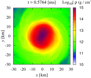
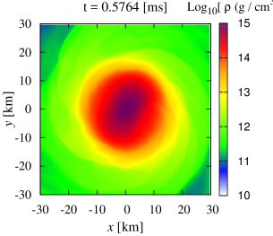
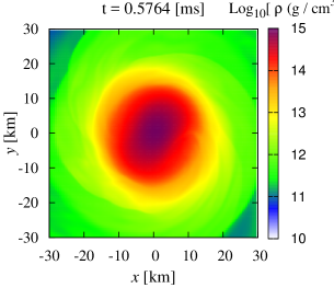
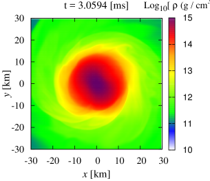
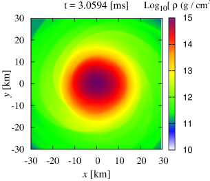
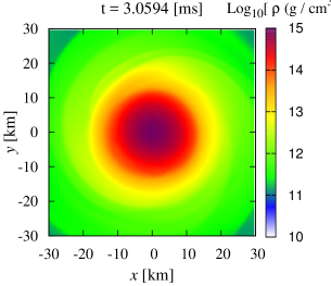
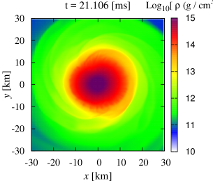
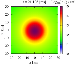
Figure 1: Evolution of rest-mass density profiles on the equatorial plane with $\alpha_{v}=0$ (left column), 0.01 (middle column), and 0.02 (right column). Each column shows three snapshots of different time: The top, middle, and bottom rows show the results for $t\approx 0$, 3, and 21 ms, respectively.

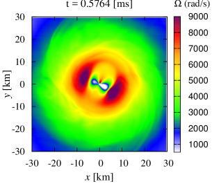
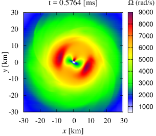
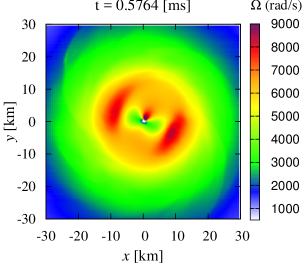
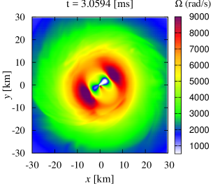
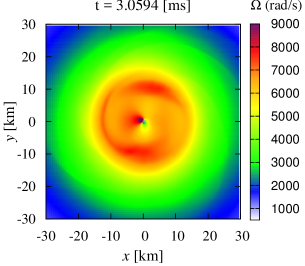
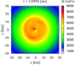
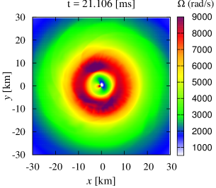
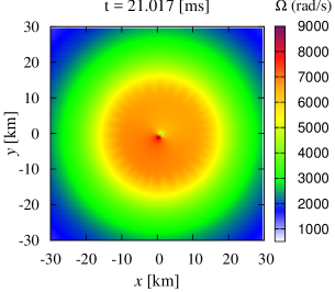
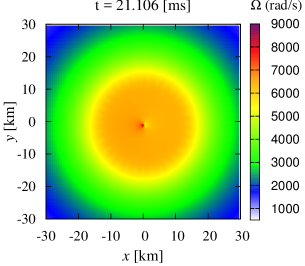
Figure 2: The same as Fig. 1 but for the angular velocity. The angular velocity is determined by $[-(y-y_{0})v^{x}+(x-x_{0})v^{y}]/[(x-x_{0})^{2}+(y-y_{0})^{2}]$ where $(x_{0},y_{0})$ is a mass center appropriately determined: $x_{0}$ and $y_{0}$ are slightly different from zero. Note that for the white region (near $(x_{0},y_{0})$), we cannot accurately determine the angular velocity.

Figures 1 and 2 display the evolution of the profiles for the rest-mass density and angular velocity on the equatorial plane, respectively. For calculating the angular velocity, we first determine the center of mass $(x_{0},y_{0})$ of the massive neutron star on the equatorial plane. Here, $x_{0}$ and $y_{0}$ are in general slightly different from zero. Then, the angular velocity is defined by $\Omega=[-(y-y_{0})v^{x}+(x-x_{0})v^{y}]/R^{2}$ where $R=\sqrt{(x-x_{0})^{2}+(y-y_{0})^{2}}$. For these figures, the left, middle, and right columns show the results for $\alpha_{v}=0$, 0.01, and 0.02, respectively. The top, middle, and bottom rows show the results for $t\approx 0$, 3, and 21 ms, respectively.

As we have always observed in the merger simulations Hotokezaka2011 ; bauswein ; Hotokezaka2013 ; takami ; tim ; ms16 ; luca , the remnants of binary neutron star mergers have a non-axisymmetric structure. In the absence of viscous effects, this non-axisymmetric structure is preserved for the timescale of $>10$ ms (see the left column of Fig. 1) because of the absence of efficient processes of angular momentum transport, and thus, the differential rotation is preserved (see the left column of Fig. 2). Note that the torque exerted by the massive neutron star of non-axisymmetric structure to surrounding material transports angular momentum outwards, but its timescale is not as short as 10 ms.

By contrast, in the presence of viscosity with $\alpha_{v}=O(10^{-2})$, the angular momentum transport process works efficiently. The middle and right columns of Fig. 2 illustrate that the angular velocity profile is modified approximately to a uniform profile for $R<15$ km in the timescale of less than 10 ms. As a result, the rest-mass density profile is also modified quickly. The middle and right columns of Fig. 1 illustrate that in a timescale of $\ll 20$ ms, the non-axisymmetric structure disappears and the remnant becomes approximately axisymmetric. The disappearance of the non-axisymmetric structure is reflected in the fact that spiral arms in the envelope disappear for $\alpha_{v}=0.01$ and 0.02 (by contrast, for $\alpha_{v}=0$, the spiral arms are continuously observed). This results from the viscous effect by which torque exerted by the remnant massive neutron star is significantly weaken due to the reduced degree of the non-axisymmetry. It is also found from Fig. 1 that in the presence of nonzero viscosity, the matter expands outwards: For $\alpha_{v}=0$, the region with $\rho\geq 10^{12}\,{\rm g/cm^{3}}$ is extended only to $R\sim 20$ km but for $\alpha_{v}=0.01$ and 0.02, it is extended to $R\sim 30$ km.

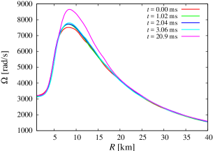
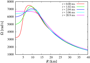
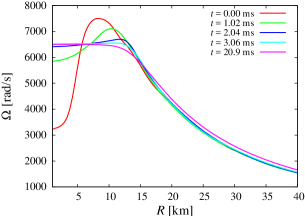
Figure 3: Averaged angular-velocity profiles along the cylindrical radius at selected time slices for the models with $\alpha_{v}=0$ (left column), 0.01 (middle column), and 0.02 (right column).

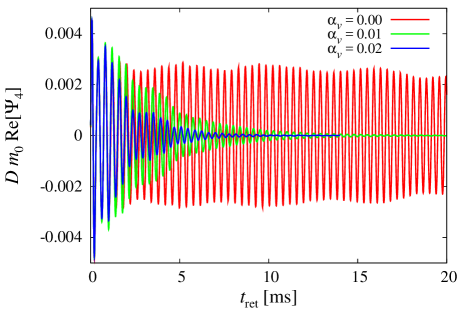
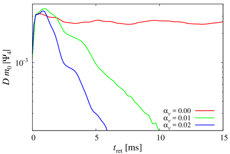
Figure 4: Left: Gravitational waveforms for $\alpha_{v}=0$, 0.01, and 0.02. Here we plot the real part of $\Psi_{4}$ for the $l=m=2$ spin-weighted spherical-harmonics component. $D$ and $m_{0}(=2.7M_{\odot})$ are the distance from the source to the observer and initial gravitational mass of the binary system. We assume that the observer of gravitational waves is located along the rotation axis of the massive neutron star. Right: Evolution of the absolute value of $\Psi_{4}$. To clarify the exponential damping of the curves, for plotting the right panel, we apply a filter to $|\Psi_{4}|$ in order to erase high-frequency noises.

Figure 3 shows the evolution of the averaged angular velocity along the cylindrical radius $R$. The averaged angular velocity is obtained by averaging $\Omega$ along the azimuthal angle $\varphi=\tan^{-1}[(y-y_{0})/(x-x_{0})]$ for fixed values of $R$ and $z$ as

$$\bar{\Omega}(R,z)={1\over 2\pi}\int_{0}^{2\pi}\Omega(R,z,\varphi)\,d\varphi.$$ (13)

As often observed in numerical relativity simulations (e.g., Ref. STU2005 ), the merger remnants are initially differentially rotating, and the maximum of the angular velocity, $\Omega$, is located in the vicinity of the stellar surface of the remnant massive neutron stars. Such profiles are formed during the merger process, because at the onset of the merger, two neutron stars with opposite velocity vectors collide with each other and kinetic energy is dissipated at their contact surfaces. In the absence of the viscous effects, this profile is preserved for a timescale longer than 20 ms. By contrast, in the presence of the viscous effects, this differential rotation disappears in the viscous timescale, $t_{\rm vis}$, because of the efficient viscous angular momentum transport. Because the peak of $\Omega$ is initially located near the stellar surface, the angular velocity near the rotation axis is increased. That is, the angular momentum is transported inward inside the massive neutron star. In this example, the rotation period of the resulting massive neutron star, $2\pi/\Omega$, is relaxed uniformly to be $\approx 1$ ms.

Associated with the viscous angular momentum transport, a massive torus surrounding the central massive neutron star develops in the presence of viscosity. The rest mass of the torus, measured for the matter with $R\geq 10$ and 15 km at $t=20$ ms, is $\approx 0.41$ and $0.19M_{\odot}$ for $\alpha_{v}=0.02$ and $\approx 0.38$ and $0.17M_{\odot}$ for $\alpha_{v}=0.01$ , respectively. The torus mass for $\alpha_{v}=0$ at $t=20$ ms is $\approx 0.26$ and $0.15M_{\odot}$ for $R\geq 10$ and 15 km, and hence, the viscous angular momentum transport enhances the massive torus formation.

As shown in Fig. 3, the torus is preserved to be differentially rotating around the central massive neutron star, and hence, it is still subject to viscous heating and viscous angular momentum transport. As indicated in our previous study SKS16 , the inner part of the torus will be heated up significantly due to the long-term viscous heating, and eventually, an outflow could be driven with a substantial amount of mass ejection. Exploring the generation processes of the outflow and mass ejection by a long-term numerical-relativity simulation is one of our future issues.

These viscous effects are reflected intensely in gravitational waves emitted by the remnant massive neutron star. Figure 4 shows the gravitational waveforms for $\alpha_{v}=0$, 0.01, and 0.02 all together. Here, we plot the real part of the out-going components of the complex Weyl scalar (the so-called $\Psi_{4}$) for the $l=m=2$ spin-weighted spherical-harmonics component. For $\alpha_{v}=0$, quasi-periodic gravitational waves are emitted for a timescale much longer than 10 ms, reflecting the fact that the non-axisymmetric structure of the massive neutron star is preserved (this waveform is essentially the same as that we found in our merger simulation Hotokezaka2013 ). The right panel of Fig. 4 clearly shows that the amplitude of gravitational waves is nearly constant for this case. By contrast, the gravitational-wave amplitude decreases exponentially in time in the viscous timescale for $\alpha_{v}\not=0$. This reflects the fact that the non-axisymmetric structure of the massive neutron star is damped in the viscous timescale. This suggests that, in the presence of MHD turbulence which would induce turbulence viscosity, the merger remnant of binary neutron stars may not emit high-amplitude gravitational waves for a timescale longer than $\sim 10$ ms.

The right panel of Fig. 4 shows that the amplitude of gravitational waves damps in an exponential manner $\propto\exp(-t/\tau)$ where $\tau$ is the $e$-holding damping timescale. In the present results, $\tau$ is approximately written as

$$\tau\approx 3.6\,{\rm ms}\left({\alpha_{v}\over 0.01}\right)^{-1}.$$ (14)

This timescale agrees approximately with the timescale for the change of the angular velocity found in Fig. 3.

We note that the author of Ref. radice recently performed a viscous hydrodynamics simulation for the merger of binary neutron stars. He also showed that the luminosity of gravitational waves decreases with the increase of the viscous coefficient, although he focused only on the case with a small viscous parameter (in the terminology of alpha viscosity, he focuses only on the cases of $\alpha_{v}=O(10^{-3})$ or less).

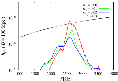
Figure 5: The spectrum of gravitational waves for $\alpha_{v}=0$, 0.01, and 0.02 with $D=100$ Mpc. We assume that the observer is located along the most optimistic direction (i.e., along the rotation axis). The spectrum, $h_{\rm eff}$, is defined by $|\tilde{h}(f)f|$ where $\tilde{h}(f)$ is the Fourier spectrum of gravitational waves. The dashed curve referred to as aLIGO denotes $[S_{n}(f)f]^{1/2}$ where $S_{n}$ is the one-sided noise spectrum density for the “Zero Detuning High Power” configuration of Advanced LIGO ligonoise .

Figure 5 plots the spectrum of gravitational waveforms defined by $h_{\rm eff}:=|f\tilde{h}(f)|$ where $\tilde{h}(f)$ is the Fourier transformation of gravitational waves defined by

$$\tilde{h}(f):=\int_{0}^{T}h(t)e^{-2\pi ift}dt.$$ (15)

Here $T$ corresponds to the final time of the simulation and $h(t)=h_{+}-ih_{\times}$ with $h_{+}$ and $h_{\times}$ denoting the plus and cross modes of gravitational waves. In numerical simulation, we obtain $\ddot{h}(t)(=\Psi_{4})$, and hence, we calculate $\tilde{h}(f)$ by

$$\tilde{h}(f)=-\int_{0}^{T}{\Psi_{4}(t)\over(2\pi f)^{2}}e^{-2\pi ift}dt.$$ (16)

Figure 5 shows that the peak amplitude decreases monotonically with the increase of $\alpha_{v}$, while the peak frequency depends only weakly on the value of $\alpha_{v}$. We note that we stopped our simulations at $t\approx 25$ ms, and hence, for $\alpha_{v}=0$ for which gravitational waves are emitted for a timescale longer than 25 ms, the peak amplitude of $\tilde{h}(f)$ would be underestimated.

To qualitatively understand the behavior on the decrease of the peak amplitude for the spectrum, we consider a simple model in which the gravitational waveforms denoted by $h:=h_{+}-ih_{\times}$ are written as a monochromatic form $A\exp(2\pi if_{p}t-\tau_{v}t)$ where $A$ is the amplitude of $h$, $f_{p}$ is the monochromatic frequency of gravitational waves, and $\tau_{v}$ denotes the damping time of the gravitational-wave amplitude (which should be proportional to $\alpha_{v}$ and approximately equal to $\tau$ in Eq. (14)). Then, at the peak of the Fourier spectrum, $f=f_{p}$, we obtain

$$|\tilde{h}(f_{p})|={1-\exp(-\tau_{v}T)\over\tau_{v}}A.$$ (17)

Thus, for $\tau_{v}T\gg 1$, $|\tilde{h}(f_{p})|=A\tau_{v}^{-1}$. Since $|\tilde{h}(f_{p})|=AT$ for $\tau_{v}\rightarrow 0$, the peak amplitude is by a factor of $(\tau_{v}T)^{-1}$ (i.e., by a factor of several) smaller than that in the non-viscous case. The numerical results agree qualitatively with this rule.

V Summary

Employing a simplified formalism for general relativistic viscous hydrodynamics that can minimally capture the effects of the shear viscous stress, we performed numerical-relativity simulations for the evolution of a remnant of binary neutron star merger, paying particular attention to gravitational waves emitted by the merger remnant. As often found in the purely hydrodynamical simulations STU2005 ; Hotokezaka2011 ; bauswein ; Hotokezaka2013 ; takami ; tim ; ms16 ; luca , in the absence of viscous effects, the merger remnant emits quasi-periodic gravitational waves for a timescale longer than 10 ms keeping their amplitude high and their frequency approximately constant. However, in the presence of viscous effects, the amplitude of gravitational waves damps in an exponential manner in time. The timescale of the exponential damping agrees approximately with the viscous timescale, which is $\lesssim 5$ ms for a plausible viscous coefficient with $\alpha_{v}\gtrsim 0.01$. This suggests that the merger remnant of binary neutron stars may not be a strong emitter of gravitational waves.

In reality, the viscous effects would be induced by MHD turbulence. Since we do not know whether the MHD turbulence is equivalent to the shear viscous-hydrodynamical turbulence, our present result is still speculative. To obtain the true answer in this problem, we have to perform an extremely-high-resolution MHD simulation in future. However, it will not be an easy task to perform such simulations in the near future because of the limitation of computational resources. Thus, the best attitude we can currently take is to keep in mind that there would be a variety of the possibilities for the evolution of the merger remnants of binary neutron stars because we have not yet fully understood the physics for the merger remnant. Thus, even if gravitational waves of a significant amplitude are not observed for the post merger phase of binary neutron star mergers in the near-future gravitational-wave observation, we should not consider that such observation implies that a massive neutron star is not formed after the merger. On the other hand, if gravitational waves of a significant amplitude are observed for the post merger phase of binary neutron star merger, we will be able to conclude that a massive neutron star is formed as a remnant and viscous effects do not play an important role for the merger remnant.

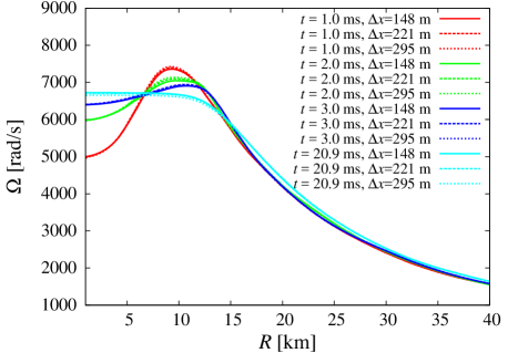
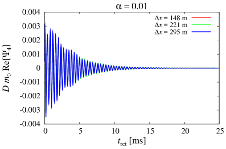
Figure 6: Left: The averaged angular velocity along the cylindrical radius at selected time slices for three different grid resolutions. Right: The gravitational waveforms for $\alpha_{v}=0.01$ with three different grid resolutions.

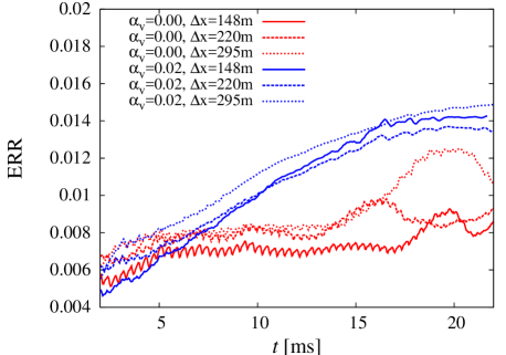
Figure 7: Evolution for the violation of the Hamiltonian constraint (ERR defined in Eq. (18)).

Appendix A Convergence and accuracy

The results shown in this paper depend only weakly on the grid resolution. To demonstrate this fact, we plot the averaged angular velocity profile and gravitational waveforms in Fig. 6. This shows that the numerical results indeed depend very weakly on the grid resolutions. The plots of Fig. 6 show that our numerical results are reliable. This result illustrates a merit of employing viscous hydrodynamics that we do not have to perform simulations with extremely high resolution in this framework, by contrast to the cases of MHD simulations.

To check the accuracy of our simulations, we also monitored the violation of the Hamiltonian constraint, denoted by $H=0$. Following our previous paper SKS16 , we focus on the following rest-mass-averaged quantity,

$${\rm ERR}={1\over M_{*}}\int\rho_{*}{|H|\over\sum_{k}|H_{k}|}d^{3}x,$$ (18)

where $H=\sum_{k}H_{k}$ and $H_{k}$ denotes individual components in $H$ composed of the energy density, the square terms of the extrinsic curvature, and three-dimensional Ricci scalar. $M_{*}$ denotes the total rest mass of the system. ERR shows an averaged degree for the violation of the Hamiltonian constraint (for ERR=0, the constraint is satisfied, while for ERR=1, the Hamiltonian constraint is by 100% violated). Figure 7 plots the evolution of ERR for $\alpha_{v}=0$ and 0.02 and for the three grid resolutions. As we showed in Ref. SKS16 , the convergence with respect to the grid resolution is lost because the spatial derivative of the velocity, which presents in the equations of $\tau_{ij}$, introduces a non-convergent error. However, the degree of the violation is kept to be reasonably small, i.e., ERR $\lesssim 0.015$, in our simulation time, irrespective of the values of $\alpha_{v}$. This approximately indicates that the Hamiltonian constraint is satisfied within 1.5% error. Therefore, we conclude that the results obtained in this paper are reliable at least in our present simulation time.

References

- (1) J. Abadie et al. Collaboration], Nucl. Instrum. Meth. A 624, 223 (2010): T. Accadia et al. Class. Quant. Grav. 28, 025005 (2011) [Erratum-ibid. 28, 079501 (2011)]: K. Kuroda, Class. Quant. Grav. 27, 084004 (2010).
- (2) P. B. Demorest et al., Nature (London) 467, 1081 (2010); J. Antoniadis et al., Science 340, 1233232 (2013).
- (3) M. Shibata, K. Taniguchi, and K. Uryū, Phys. Rev. D 71, 084021 (2005): M. Shibata and K. Taniguchi, Phys. Rev D 73, 064027 (2006).
- (4) K. Hotokezaka, K. Kyutoku, H. Okawa, M. Shibata, and K. Kiuchi, Phys. Rev. D 83, 124008 (2011).
- (5) A. Bauswein and H.-Th. Janka, Phys. Rev. Lett. 108, 011101 (2012).
- (6) K. Hotokezaka, K. Kiuchi, K. Kyutoku, T. Muranushi, Y. -I. Sekiguchi, M. Shibata and K. Taniguchi, Phys. Rev. D 88, 044026 (2013).
- (7) K. Takami, L. Rezzolla, and L. Baiotti, Phys. Rev. D 91, 064001 (2015).
- (8) T. Dietrich, S. Bernuzzi, M. Ujevic, and B. Brügmann, Phys. Rev. D 91, 124041 (2015).
- (9) M. Shibata, Numerical Relativity (World Scientific Publishing Co., 2016).
- (10) L. Baiotti and L. Rezzolla, Rep. Prog. Phys. to be published (arXiv: 1607.03540).
- (11) D. J. Price and S. Rosswog, Science 312, 719 (2006).
- (12) K. Kiuchi, K. Kyutoku, Y. Sekiguchi, M. Shibata, and T. Wada, Phys. Rev. D 90, 041502(R) (2014); K. Kiuchi, P. Cerda-Duran, K. Kyutoku, Y. Sekiguchi, and M. Shibata, Phys. Rev. D 92, 124034 (2015).
- (13) S. A. Balbus and J. F. Hawley, Rev. Mod. Phys. 70, 1 (1998).
- (14) J. F. Hawley, S. A. Richers, X. Guan, and J. H. Krolik, Astrophys. J. 772, 102 (2013).
- (15) T. K. Suzuki and S. Inutsuka, Astrophys. J. 784, 121 (2014).
- (16) J. M. Shi, J. M. Stone, and C. X. Huang, Mon. Not. R. Soc. Astron. 456, 2273 (2016): G. Salvesen, J. B. Simon, P. J. Armitage, and M. C. Begelman, Mon. Not. R. Soc. Astron. 457, 857 (2016).
- (17) M. D. Duez, Y.-T. Liu, S. L. Shapiro, and B. C. Stephens, Phys. Rev. D 69, 104030 (2004).
- (18) D. Radice, Astrophys. J. Lett. 838, L2 (2017) (arXiv: 1703.02046).
- (19) M. Shibata, K. Kiuchi, and Y. Sekiguchi, Phys. Rev. D 95, 083005 (2017).
- (20) W. Israel and J. M. Stewart, Ann. Phys. 118, 341 (1979).
- (21) W. A. Hiscock and L. Lindblom, Annals of Physics, 151, 466 (1983).
- (22) L. D. Landau and E. M. Lifshitz, Fluid Mechanics (Peragamon Press, London, 1959).
- (23) N. I. Shakura and R. A. Sunyaev, Astron. Astrophys. 24, 337 (1973): S. L. Shapiro and S. A. Teukolsky, Black holes, White dwarfs, and Neutron stars: the Physics of Compact Objects (Wiley, 1983), chapter 14.
- (24) M. Shibata and T. Nakamura, Phys. Rev. D 52, 5428(1995): T. W. Baumgarte and S. L. Shapiro, Phys. Rev. D 59, 024007(1998): M. Campanelli, C. O. Lousto, P. Marronetti, and Y. Zlochower, Phys. Rev. Lett. 96, 111101 (2006): J. G. Baker, J. Centrella, D.-I. Choi, M. Koppitz, and J. van Meter, Phys. Rev. Lett. 96, 111102 (2006).
- (25) N. K. Glendenning and S. A. Moszkowski, Phys. Rev. Lett. 67, 2414 (1991).
- (26) J. S. Read, B .D. Lackey, B. J. Owen, and J. L. Friedman, Phys. Rev. D 79, 124032 (2009).
-
(27)
https://dcc.ligo.org/cgi-bin/DocDB/
ShowDocument?docid=2974