Summed Parallel Infinite Impulse Response (SPIIR) Filters For Low-Latency Gravitational Wave Detection

Abstract

With the upgrade of current gravitational wave detectors, the first detection of gravitational wave signals is expected to occur in the next decade. Low-latency gravitational wave triggers will be necessary to make fast follow-up electromagnetic observations of events related to their source, e.g., prompt optical emission associated with short gamma-ray bursts. In this paper we present a new time-domain low-latency algorithm for identifying the presence of gravitational waves produced by compact binary coalescence events in noisy detector data. Our method calculates the signal to noise ratio from the summation of a bank of parallel infinite impulse response (IIR) filters. We show that our summed parallel infinite impulse response (SPIIR) method can retrieve the signal to noise ratio to greater than 99% of that produced from the optimal matched filter. We emphasise the benefits of the SPIIR method for advanced detectors, which will require larger template banks.

I Introduction

The interferometric gravitational wave (GW) detectors LIGO LIG , and Virgo VIR have reached a sensitivity at which the detection of GWs is possible. The LIGO detectors are currently undergoing a major upgrade to Advanced LIGO, for which the sensitivity will be improved ten fold relative to Initial LIGO Smith and for the LIGO Scientific Collaboration (2009). Hence Advanced LIGO will be able to detect GW (GW) sources within a volume of space one thousand times larger than that of initial LIGO, out to $\sim$200-300$\,\mathrm{Mpc}$ Adv (2007).

The emission of GWs produced by compact binary coalescence (CBC) can be modelled with a high degree accuracy Abbott et al. (2009). When two compact bodies, such as neutron stars or black holes are in orbit, Einstein’s equations predict the generation of GWs. As the bodies spiral towards each other a GW is created that increases in frequency over time until the bodies merge, following what is known as the inspiral waveform. Ground based detectors have frequency passbands that allow them to be sensitive to the final stages of such events up to a total system masses of several hundred $M_{\odot}$.

Neutron star binary mergers are widely thought to be the progenitors of short hard gamma-ray bursts (short GRBs) Fox et al. (2005); Nakar (2007). The delay between the final GW emission and the onset of the GRB is estimated to be as short as 0.1 seconds or as long as tens to hundreds of seconds van Putten (2009); Zhang and Mészáros (2004). The electromagnetic emission of the GRB event is not well understood. Related to the initial GRB there is thought to be a prompt emission in the X-ray and optical wavelengths followed by a delayed afterglow of cascading wavelengths. Prompt optical emission may occur tens to hundreds of seconds after the initial burst. The low-latency detection of the GW associated with a neutron star merger could lead to the localisation of a GRB source event on the sky, enabling fast moving telescopes to observe the prompt optical emission. Data collected from a multitude of sources — GWs, gamma-rays, X-rays and optical counterparts of the GRB — will lead to maximum insight into these highly energetic events.

The standard strategy for searching for the existence of inspiral waveforms in the detector data is based on matched filtering Abbott et al. (2009) (and references therein). This method, based on Wiener optimal filtering, is a correlation of an expected inspiral waveform template and the detector data, weighted by the inverse noise spectral density of the detector Wainstein and Zubakov (1962). In order to save computational costs, this correlation is performed in the frequency domain, via a Fourier transform of a finite segment of detector data. In previous LIGO searches, the detector data is split up into “science blocks”, which are further divided into “data segments” chosen to be at least twice the length of the longest waveform in the template bank Abbott et al. (2008). Each proceeding data segment is chosen to overlap the previous one by 50%. Each segment therefore must be matched filtered in a time that is half the length of the segment for a real-time analysis, that is, the filter output rate is equal to the data input rate. In this case, the matched filter process has a minimum latency (from signal arrival to signal detection) that is proportional to the longest template (see Luan (2011) for more details). Advanced LIGO will have an increased bandwidth over Initial LIGO, with the lower bound dropping from 40$\,\mathrm{Hz}$ to 10$\,\mathrm{Hz}$ Adv (2007). GW signals from CBC events spend much more time at these lower frequencies. Hence waveforms used for matched filtering in Advanced LIGO will be much longer (1000s of seconds). This in turn means the segment length will be increased, further increasing the latency. The latency of this method to produce GW triggers is longer than the time to onset of prompt optical emission after coalescence (10s to 100s of seconds). After this amount of time, the early electromagnetic counterpart of a GRB event will be significantly faded, and may be missed by telescopes altogether.

A low-latency GW detection method is required to trigger follow-up electromagnetic observations of the prompt optical emission. So far two frequency domain methods have been developed to solve this issue. The VIRGO group has produced a low-latency pipeline based on Multi-Band Template Analysis (MBTA) Buskulic et al. (2010), and LIGO is also working on a new method, Low-Latency On-line Inspiral Data analysis (LLOID) method. In MBTA the matched filtering technique is split over two frequency bands, and the output is coherently added, reducing latency. A latency of less than 3 minutes until the availability of a trigger using this method has been achieved Buskulic et al. (2010). Low-latency in the LLOID method is achieved by first down-sampling the incoming data into multiple streams and then applying frequency domain finite impulse response (FIR) filters gst . The computational cost of this pipeline is reduced by decreasing the number of templates via singular value decomposition Cannon et al. (2010).

We introduce a new method to detect CBC signals in the time domain using infinite impulse response (IIR) filters. Approximating an inspiral waveform by a summation of time shifted exponentially increasing sinusoids enables us to construct a bank of parallel single-pole IIR filters. Each IIR filter acts as a narrow bandpass filter. When each appropriately delayed IIR filter is added the coherent output approximates the matched filter output of the exact waveforms. We call this the summed parallel infinite impulse response (SPIIR) method. Figure 1 visually demonstrates the idea of using a bank of IIR filters as narrow bandpass filters.

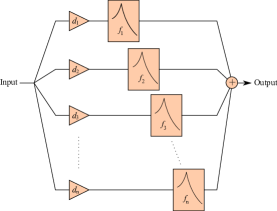
Figure 1: A schematic overview of the SPIIR method. The input is split into different channels, time delayed by an amount $d$, then passed through a narrow bandpass IIR filters, each with a different central frequency $f$. Finally the output of each individual IIR filter is summed, giving the output of the SPIIR method.

For a full explanation of the mathematical principles, see Luan (2011). In this follow up paper, we numerically address the issues essential to the practical use of this method for the upcoming advanced detectors. We calculate the filter coefficients and demonstrate via numerical simulations how well our method approximates the optimal matched filter as a function the number of filters per bank using a range of parameters. We also show that the detection rate of the SPIIR method is very similar to that of the matched filter method. It has been shown theoretically that in order to get the same latency as the SPIIR method, the frequency domain matched filter method would require greater computational resources Luan (2011).

The structure of this paper is as follows: In section II we will go through the formal introduction of the inspiral waveform and matched filtering, and how to get from the continuous frequency domain matched filter to the time domain discrete matched filter. This will lead to a demonstration on how it is possible to approximate an inspiral signal by a sum of exponentially increasing sinusoids. The methodology is explained in Section III and will cover how we set up our simulation to test the efficiency of the SPIIR method as opposed to the frequency domain matched filter. Section IV will analyse the results of the simulation and Section V will discuss the implications of these results for advanced detectors.

II Methodology

Gravitational wave interferometers output the strain induced by gravitational waves incident on the detector, as well as inherent noise. In unitless strain, the detector output will be,

$$s(t)=\begin{cases}n(t)&\text{if signal is absent}\\ n(t)+h(t)&\text{if signal is present}\end{cases}$$ (1)

where $n(t)$ is the noise inherent in the detector. The sensitivity of the instrument can be characterized by the (one-sided) strain power spectral density $S_{n}(f)$,

$$\left\langle\tilde{n}(f)\tilde{n}^{*}(f^{\prime})\right\rangle=\frac{1}{2}S_{n}(f)\delta(f-f^{\prime})$$ (2)

where the tilde represents the forward Fourier transform,

$$\tilde{q}(f)=\int_{-\infty}^{\infty}q(t)e^{-2\pi ift}dt.$$ (3)

II.1 The Inspiral Waveform

The gravitational-wave strain incident at the interferometer is given by

$$h(t)=F_{+}(\theta,\phi,\psi)h_{+}(t)+F_{\times}(\theta,\phi,\psi)h_{\times}(t)$$ (4)

where the detector response functions $F_{+}$ and $F_{\times}$ are functions of $(\theta,\phi)$ - the standard spherical polar coordinates measured with respect to the Earth’s fixed frame, and $\psi$ is the polarisation angle. The detector response function can be found in Anderson et al. (2001). The $+$ and $\times$ polarisations of the waveform are,

$$h_{+}(t) =\left(\frac{1+\cos^{2}\iota}{2}\right)A(t)\cos\phi(t)$$ (5)

$$h_{\times}(t) =\left(\cos\iota\right)A(t)\sin\phi(t)$$ (6)

For non-spinning binaries with a chirp mass $\mathcal{M}=((m_{1}m_{2})^{3}/(m_{1}+m_{2}))^{1/5}$ in the range of $1-3M_{\odot}$ — we will hereafter assume — the waveforms can be modelled to very high accuracy using the Restricted post-Newtonian (PN) expansion Abbott et al. (2004); Blanchet et al. (1995, 1996) in the LIGO band (assumed to be 10-1500 $\,\mathrm{Hz}$ for advanced LIGO). For restricted waveforms, only the leading order of the amplitude $A(t)$ is taken,

$$A(t) =\frac{G\mathcal{M}}{Dc^{2}}\left(\frac{t_{c}-t}{5G\mathcal{M}/c^{3}}\right)^{-1/4}$$ (7)

and the post-Newtonian phase $\phi(t)$ is given by

$$\phi(t) =\phi_{c}-2\left(\frac{t_{c}-t}{G\mathcal{M}/c^{3}}\right)^{5/8}+\mbox{higher order terms}$$ (8)

In addition to the source masses $m_{1},m_{2}$, there are several unknown parameters; the time of coalescence $t_{c}$, the phase at coalescence $\phi_{0}$, distance from observer to source $D$, the inclination angle of the binary’s orbital plane relative the line of sight $\iota$, and the polarisation angle $\psi$. However by using the linear combination trigonometric identity, one can re-express the strain (4) by splitting the scaling factor due to distance, sky location and orientation to the mass dependant time evolution of the waveform Fairhurst and Brady (2008),

$$h(t) =\frac{1\,\mathrm{Mpc}}{D_{\rm eff}}\left[h_{c}(t)\cos\phi_{0}+h_{s}(t)\sin\phi_{0}\right]$$ (9)

where the scalar factor $D_{\rm eff}$ is,

$$D_{\rm eff}=\frac{D}{\sqrt{F_{+}^{2}\left(1+\cos^{2}\iota\right)^{2}/4+F_{\times}^{2}\left(\cos\iota\right)^{2}}}$$ (10)

which gives $\phi_{0}$, an unknown phase as,

$$\phi_{0}=\phi_{c}+\arctan\frac{F_{\times}\left(2\cos\iota\right)}{F_{+}\left(1+\cos^{2}\iota\right)}$$ (11)

We now define the terms $h_{c}$ and $h_{s}$ as the waveform at $\phi_{0}=0$ and $\phi_{\pi/2}$, scaled at 1$\,\mathrm{Mpc}$ as the so called “cosine” and “sine” phases Brady and Fairhurst (2008),

$$h_{c}(t) =A_{1\,\mathrm{Mpc}}(t)\cos\phi(t)$$ (12)

$$h_{s}(t) =A_{1\,\mathrm{Mpc}}(t)\sin\phi(t)$$ (13)

II.2 The Matched Filter

The matched filter $Q$ is a linear operator that maximises the ratio of “signal” to “noise” present in the detector data $s$ Allen et al. (2005). It is denoted by,

$$z(t) =2\int_{-\infty}^{\infty}\frac{\tilde{s}(f)\tilde{Q}^{*}(f)}{S_{n}(|f|)}e^{2\pi ift}df=\left(s(t)\left|Q\right)\right.$$ (14)

Where we have also defined the inner product $\left(a\left|b\right)\right.$. The signal to noise ratio (SNR) is generally defined as the ratio of observed filter output to it’s expected root-mean square flucations or standard deviation,

$$\mathrm{SNR} =\frac{z}{\sqrt{\left\langle(z-\left\langle z\right\rangle)^{2}\right\rangle}}=\frac{z}{\sqrt{\left\langle z\right\rangle^{2}}}=\frac{z}{\sqrt{\left(Q\left|Q\right)\right.}}$$ (15)

Note that in the absence of a signal, $\left\langle\mathrm{SNR}\right\rangle=0$ and $\left\langle(\mathrm{SNR})^{2}\right\rangle=1$ independent of the normalisation of the filter $Q$.

II.3 Two-Phase Filter

A convenient way to search for the unknown phase constant $\phi_{0}$ is to filter both phases $h_{c}$ and $h_{s}$ separately and then combined to form a complex signal. The two-phase filter is defined as,

$$z(t) =\left(s(t)\left|h_{c}\right)\right.+i\left(s(t)\left|h_{s}\right)\right.$$ (16a)

$$\begin{split}&=2\int_{-\infty}^{\infty}\frac{\tilde{s}(f)\tilde{h}_{c}^{*}(f)}{S_{n}(f)}e^{2\pi ift}df\\ &\qquad\qquad+i2\int_{-\infty}^{\infty}\frac{\tilde{s}(f)\tilde{h}_{s}^{*}(f)}{S_{n}(|f|)}e^{2\pi ift}df\end{split}$$ (16b)

The advantage of using the phases $h_{c,s}$ is that in the stationary phase approximation Droz et al. (1999), $h_{c}$ and $h_{s}$ are exactly orthogonal ($\left(h_{c}\left|h_{s}\right)\right.=\left(h_{s}\left|h_{s}\right)\right.$, $\left(h_{c}\left|h_{s}\right)\right.=0$). It then follows, $\tilde{h}_{c}(f)=i\tilde{h}_{s}(f)$ for $f>0$. Generally, this is applied to (16) to give the two-phase matched filter as,

$$z(t) =4\int_{0}^{\infty}\frac{\tilde{s}(f)\tilde{h}_{c}^{*}(f)}{S_{n}(|f|)}e^{2\pi ift}df$$ (17)

However in this paper, we prefer to maintain the form of the two-phase filter in (16). In convention with the field, the amplitude signal to noise ratio of the (quadrature) matched filter is defined as the absolute value of the two-phase filter, divided by a normalisation constant that is equal to standard deviation of the real and imaginary parts of the two-phase filter,

$$\rho(t)=\frac{|z(t)|}{\sigma}$$ (18)

where $\sigma^{2}$ is,

$$\sigma^{2}=2\int_{-\infty}^{\infty}\frac{\left|\tilde{h}_{c}(f)\right|^{2}}{S_{n}(f)}df=\left(h_{c}\left|h_{c}\right)\right.$$ (19)

Note that in the in the absence of a signal (just noise), the SNR $\rho$ (18) is Rayleigh distributed with mean $\sqrt{\pi/2}$ and variance $1$, which is identical to the Chi-distribution with two degrees of freedom (one for each of the phases). This of course implies that the SNR squared, $\rho^{2}$ is Chi-square distributed with two degrees of freedom. Hence the probability of finding an SNR value greater than $\rho_{*}$ is Brady and Fairhurst (2008),

$$P(\rho^{2}>\rho_{*}^{2})=e^{-\rho_{*}^{2}/2}.$$ (20)

II.4 Digital Time Domain Filtering

The two-phase matched filter 16 is a cross correlation of phase $h_{c,s}(t)$ and the detector output $s(t)$, weighted by the inverse noise spectral density $S_{n}(f)$. By defining the quantity $x$ as the over-whitened strain data,

$$x(t)=\int_{-\infty}^{\infty}\frac{\tilde{s}(f)}{S(f)}e^{2\pi ift}df$$ (21)

we can use the cross-correlation theorem to define the two-phase matched filter in the time domain,

$$z(t) =2\int_{-\infty}^{t}x(t^{\prime})h_{c}(t^{\prime}-t)dt^{\prime}+i2\int_{-\infty}^{t}x(t^{\prime})h_{s}(t^{\prime}-t)dt^{\prime}$$ (22)

$$=2\int_{-\infty}^{t}x(t^{\prime})\hat{h}(t^{\prime}-t)dt^{\prime}$$ (23)

where $\hat{h}=h_{c}(t)+ih_{s}(t)=A(t)e^{i\phi(t)}$.

The discrete form of the continuous time domain matched filter (23) is,

$$z_{k}=2\sum_{j=-\infty}^{k}x_{j}\hat{h}_{j-k}\Delta t$$ (24)

where $t=k\Delta t$. In practise, the inspiral waveform template $h_{i}$ is bounded (because the detector is only sensitive over a bandwidth), and the summation becomes finite, making this a finite impulse response (FIR) filter.

II.5 Infinite Impulse Response Filter

Now let us introduce an alternative digital filter, the infinite impulse response (IIR) filter. The difference equation of a general IIR filter is,

$$y_{k}=\sum_{n=1}^{N}a_{n}y_{k-n}+\sum_{m=0}^{M}b_{m}x_{k-m}$$ (25)

where $y_{k}$ is the filter output at time step $k$, ($t=k\Delta t$), $x_{k}$ is the filter input, and $a$’s and $b$’s are complex coefficients.

Examples of IIR filters in common usage are Chebyshev, Butterworth and elliptic filters. IIR filters use much less computational resources than an equivalent FIR filter. This is because they have “memory” — the previous outputs are fed back into the filter. However digital IIR filter design is a more complex process than FIR design. Obtaining the coefficients is usually done by first constructing an equivalent analog filter and applying well-known methods, such as the bi-linear transform or impulse invariance. Multiple IIR filters used together have different forms, such as direct form I & II, cascade (series) and parallel. In a series configuration, the overall transfer function is the multiplication of each IIR filter transfer function. In a parallel bank of IIR filters, where the output is summed together, the overall transfer function is the summation of the different transfer functions.

First, let’s analyse the simplest single-pole IIR filter. The difference equation of this filter is

$$y_{k}=a_{1}y_{k-1}+b_{0}x_{k}.$$ (26)

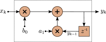
Figure 2: A signal processing schematic showing the flow of data through a digital single-pole IIR filter. The input, $x_{k}$ is multiplied by a complex constant $b_{0}$, then added to the previous output that has been multiplied by another complex constant $a_{1}$, resulting in the current output $y_{k}$. It should be noted that this filter, in principle, should be have been run forever.

A solution to this first-order linear inhomogeneous difference equation is

$$y_{k}=\sum_{j=-\infty}^{k}x_{j}b_{0}a_{1}^{k-j}.$$ (27)

By defining the complex coefficient $a_{1}$ in the form,

$$a_{1}=e^{-(\gamma+i\omega)\Delta t}$$ (28)

and comparing (24) and (27), it is easy to see that the output of the simple filter (26) is the cross-correlation of $x_{k}$ and complex sinusoid $u_{n}$ with frequency $\omega$ and a magnitude that increases with an exponential factor $\gamma$ for $n<0$:

$$u_{n}=b_{0}e^{(\gamma+i\omega)n\Delta t}\Theta(-n)$$ (29)

where $\Theta(-n)$ is the Heaviside function.

II.6 Approximation to an inspiral waveform

Since $\phi(t)$ is not linear in time, a complex sinusoid (29) cannot approximate the $h_{c,s}$ phases of the inspiral waveform $\hat{h}(t)=A(t)e^{i\phi(t)}$. However we can easily linearise the phases by a first-order Taylor expansion about the time $t_{l}^{*}$:

$$A(t)e^{i\phi(t)}\simeq A(t_{l}^{*})e^{i\phi(t_{l}^{*})+i\dot{\phi}(t_{l}^{*})(t-t_{l}^{*})};$$ (30)

since the amplitude $A(t)$ does not increase at the same rate as $\phi(t)$, only a linear expansion of $\phi(t)$ is required. Multiplying by the window function $e^{\gamma_{l}(t-t_{l})}\Theta(t_{l}-t)$ makes this approximation an exponentially increasing constant frequency complex sinusoid with cutoff time $t_{l}$:

$$u_{l}(t) =A(t_{l}^{*})e^{i(\phi(t_{l}^{*})+\dot{\phi}(t_{l}^{*})(t_{l}-t_{l}^{*}))}e^{(\gamma_{l}+i\dot{\phi}(t_{l}^{*})(t-t_{l})}\Theta(t_{l}-t).$$ (31)

The expansion point $t_{l}^{*}$ is chosen to be near the cutoff time, $t_{l}^{*}=t_{l}-\alpha T_{l}$, where $\alpha$ is a tunable parameter and the interval $T_{l}$ is the duration in which the approximation is valid:

$$|\frac{1}{2}\ddot{\phi}(t_{l})T_{l}^{2}|=\epsilon<1$$ (32)

and $\epsilon$ is a tunable parameter chosen to be to small. Equation (31) implies that the coefficient $b_{0}$ for the $l$th complex sinusoid is,

$$b_{0,l} =A(t_{l}^{*})e^{i(\phi(t_{l}^{*})+\dot{\phi}(t_{l}^{*})(t_{l}-t_{l}^{*}))}$$ (33)

and the frequency $\omega_{l}=\dot{\phi}(t_{l}^{*})$.

In this paper, we chose the cutoff time $t_{l}$ of the first sinusoid to correspond to the time at which the waveform has the highest frequency detectable by the LIGO detector band. The next sinusoid is chosen by moving to an earlier time, $t_{l+1}=t_{l}-T_{l}$. Since we want the $l$th sinusoid to be mostly present on the interval $t_{l}-T_{l}<t<t_{l}$, we choose the damping factor to be $\gamma_{l}=\beta/T_{l}$, where $\beta$ is a tunable parameter. This procedure is repeated until the time $t_{l}$ corresponds to a time in the waveform that has frequency below the LIGO detector band. Hence the number of sinusoids is dependent on the value of $\epsilon$, the rate of frequency change ($\ddot{\phi}(t)$), which is dependent on the masses of the system, and the detector bandwidth. For more information on this procedure, see Luan (2011).

We can now approximate the phases $\hat{h}(t)=A(t)e^{i\phi(t)}$ by an addition of a series of damped sinusoids $u(t)$ with cutoff times $t_{l}$:

$$A(t)e^{i\phi(t)}\simeq U(t) =\sum_{l}u_{l}(t)$$

$$=\sum_{l}b_{0,l}e^{(\gamma_{l}+i\omega_{l})(t-t_{l})}\Theta(t_{l}-t).$$ (34)

Figure 3 shows an illustration of how damped constant frequency sinusoids can add to give an inspiral like waveform.

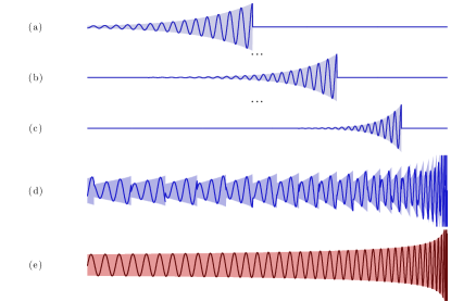
Figure 3: An illustrative diagram demonstrating the ability to linearly sum exponentially increasing constant frequency sinusoids to approximate an inspiral like waveform. The top three panels (a-c) show three example sinusoids with different damping, frequency and cutoff time factors. Panel (d) shows the linear addition of all the sinusoids (at different scales). Panel (e) shows the exact inspiral-like waveform. Note that this figure is only for illustrative purposes.

II.7 Summed Parallel IIR filtering

Each complex sinusoid $u_{l}(t)$ in equation (II.6) can be searched for in the data $x$ using the single pole IIR filter (26). Here the cutoff time is incorporated by running each filter on a delay, $d_{l}=t_{l}/\Delta t$. The output of the $l$th filter at time $k$ is

$$y_{k,l}=a_{1,l}y_{k-1,l}+b_{0,l}x_{k-d_{l}}.$$ (35)

The linear summation of the output of all filters is the cross-correlation of the data $x$ and the approximate waveform $U(t)$ in (II.6):

$$z_{k}\simeq 2\Delta t\sum_{l}y_{k,l}.$$ (36)

Here $z$ is equivalent to the value computed by the discrete time domain two phase filter (24) when using a template $\hat{h}(t)=U(t)$. From equation (18), it follows that the absolute value of the summation (36) divided by $\sigma_{U}$ is the SNR, which we term the output of the Summed Parallel Infinite Impulse Response (SPIIR). The normalisation factor $\sigma_{U}$ is defined as

$$\sigma_{U}^{2}=4\int_{0}^{\infty}\frac{\left|\tilde{U}_{\Re}(f)\right|^{2}}{S_{n}(f)}df.$$ (37)

Where $\tilde{U}_{\Re}(f)$ is the Fourier transform of the real part of $U(t)$, (which approximates $h_{c}(t)$). The similarity of the SPIIR output and the matched filter output will depend on how well $U(t)$ approximates the given template.

III Implementation for Performance Testing

III.1 IIR bank construction

To confirm the ability of the SPIIR method to recover a good SNR, it is first required to show that the approximate inspiral waveform (II.6) is a good “match” to the theoretical inspiral waveform (9). We define the overlap $\Delta$ as the inner product of the approximate waveform $U$ and the template $h$:

$$\Delta=\left(\frac{h}{\sqrt{\left(h\left|h\right)\right.}}\left|\frac{U}{\sqrt{\left(U\left|U\right)\right.}}\right)\right.=\frac{\left(h\left|U\right)\right.}{\sqrt{\left(h\left|h\right)\right.\left(U\left|U\right)\right.}}$$ (38)

We initially approximate a canonical 2PN 1.4-1.4 $M_{\odot}$ inspiral waveform band limited to 10-1500$\,\mathrm{Hz}$ using the value of the tunable parameters $\epsilon$, $\alpha$ and $\beta$ to be consistent with the high overlap results of Luan (2011). With some minor variation of their values, we aim to recover the highest overlap possible. Once a good choice of $\alpha$ and $\beta$ is found for the 2PN 1.4-1.4 $M_{\odot}$ template, we use the same values for other templates, but vary the value $\epsilon$ (and consequently the number of IIR filters in each bank) to see the effect on overlap.

III.2 Detector Data Simulation

To test the detection efficiency of the SPIIR method compared to the frequency domain matched filter, we will filter two mock signals, one for which the input data is just LIGO-like noise, and the other with the same noise plus an inspiral waveform injection scaled to represent a source at a chosen effective distance $D_{\rm eff}$.

For this test, we need to construct a finite segment of detector data to filter. Because of the IIR filters should in principle should be run for an infinite length of the input data, we need to run the IIR bank for a finite “warm-up” period before the output is consistent with that of an IIR filter that has been running for an infinite amount of time. In practise, we choose to run each filter for 2 $e$-foldings of time before we accept the output as being identical to one which has run for an infinite amount of time. Additionally, since each IIR filter in the bank runs on a delay, the summed output of all the IIR filters will not be produced until after the longest delay time ($d_{\rm max}$) has passed. The filter that has the longest delay ($d_{\rm max}$) is also the one that has the longest decay rate $\gamma_{\rm max}$. In total, the input data must at least $d_{\rm max}+2\gamma_{\rm max}^{-1}$ in length before any output is produced. Hence the length of the input data is,

$$N_{\rm input}=d_{\rm max}+2\gamma_{\rm max}^{-1}+N_{\rm analysis}$$ (39)

where $N_{\rm analysis}$ is the length of analysis period, which we choose to be 4 seconds. Hence the 4$\,\mathrm{s}$ SPIIR output will tell us whether there is an injection that ended somewhere within those 4 seconds. At a sample rate of 4096$\,\mathrm{Hz}$, the analysis period is $N_{\rm analysis}=16834$ data points long. In our simulation, we find $d_{\rm max}=4081683$ and $2\gamma_{\rm max}^{-1}=149432$, resulting in $N_{\rm input}=4247499$.

III.2.1 Noise generation

The LIGO-like noise data is produced by creating a normally distributed white noise time series of length $N_{\rm input}$, then colouring it by the theoretical advanced LIGO noise spectrum $S_{n}(f)$ A. We then over-whiten this time series using equation (21) to produce the waveform-free noise input data $x$:

$$x_{\rm noise}(t)=n^{\rm ow}(t).$$ (40)

III.2.2 Waveform injection

We create our waveform injections by first producing an inspiral waveform band-limited between 10 and 1500$\,\mathrm{Hz}$. The injection is padded with zeros so that it has the length $N_{\rm input}$. The end of the waveform is chosen so that it finishes somewhere after $d_{m}+2\gamma_{m}^{-1}$ data points. The injection signal is then over whitened using equation (21). The over-whitened injection can then be placed in the over-whitened noise signal,

$$x_{\rm noise+injection}(t)=x_{\rm noise}(t)+h^{\rm ow}(t).$$ (41)

III.2.3 Matched filter comparison

As a comparison, we will also perform a frequency domain correlation matched filter. For this process, since the input data is already over-whitened, it only needs to be cross-correlated with the waveform. Section II.2 outlines how this is done. The cosine phase $h_{c}(t)$ gets pre-padded with enough zeros to get to length $N_{\rm input}$. This ensures that $\tilde{h}_{c}(f)$ has the same spectral resolution as $\tilde{s}(f)$. The matched filter (17) produces a time series of $N_{\rm input}$ length. However the first $N_{\rm input}-N_{\rm analysis}$ data points are erroneous wrap-around caused by the FFT. Only the interval $[N_{\rm input}-N_{\rm analysis}+1,N_{\rm analysis}]$ is used to determine if a waveform is present.

III.3 Detection Efficiency

To test the detection efficiency of the SPIIR method compared to the traditional matched filter method we will construct several receiver operating characteristic (ROC) curves for 2PN 1.4-1.4 $M_{\odot}$ waveforms injected for different effective distances $D_{\rm eff}$. To create each ROC curve, we first find the false alarm rate. The false alarm rate is found by realising an $N_{\rm input}$ length LIGO-like noise time series, filtering this input data, and analysing the output of the 4$\,\mathrm{s}$ analysis period (the SNR). We will count this realisation as a false positive if at any point within the 4 seconds the SNR goes over a given SNR threshold. Several thresholds will be chosen, giving the false positive as a function of threshold. After $>10^{6}$ noise realisations, the false alarm rate is simply the ratio of total number of false positives to number of noise realisations. Likewise, to see if the IIR filter doesn’t miss too many true positives, we inject a 2PN 1.4-1.4 $M_{\odot}$ waveform using the prescribed method in III.2.2 for a given $D_{\rm eff}$ into LIGO-like noise. After filtering, if at any point within the analysis period the SNR is above a given threshold, this realisation is counted as a true positive. Again, after $>10^{6}$ noise realisations, we calculate the detection rate as a ratio of the total number of true positives to number of realisations. The plot of false alarm rate versus detection rate gives the ROC curve.

IV Results

IV.1 Inspiral Waveform Overlap

Starting with the canonical 1.4-1.4 $M_{\odot}$ second order post-Newtonian binary waveform band limited to be between 10 and 1500 $\,\mathrm{Hz}$ we found, using the parameters $\epsilon=0.04$, $\alpha=0.99$, $\beta=0.25$ in the procedure outlined in Section II.6, that can recover an overlap of 99% using 687 IIR filters.

We find that increasing the value of $\epsilon$ will in general increase the overlap, as the frequency space is more finely sampled. However there seems to be a limit, as the damping factor $\gamma$ causes the adjacent IIR filters to run into each other.

With this choice of $\alpha$ and $\beta$ we are able to recover a high overlap for different mass pairs as well. Figure 4 shows the overlap as a function of number of IIR filters for six different mass pairs.

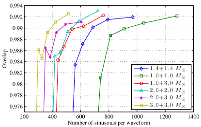
Figure 4: The overlap between the exact inspiral waveform and the approximate inspiral waveform as a function of number of damped sinusoids. In general the greater the number of sinusoids per waveform, the greater the overlap. However the choice of $\gamma_{l}$s greatly affects the overlap.

IV.2 Ability to Recover SNR

Figure 5 shows the SNR produced from both the matched filter technique and the SPIIR method. The input time series is constructed following Section III.2. The injection of a 2PN 1.4-1.4 $M_{\odot}$ waveform scaled for an effective distance of 250$\,\mathrm{Mpc}$ is added to LIGO-like noise. The $x$-axis of the plot is centred about end of the injection ($t=\tau_{c}$), which is directly in the middle of the analysis period. Around this time, the SNR peaks to 8.2, which is near the expected value of 7.9 for an injection at this distance.

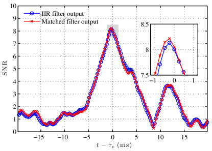
Figure 5: The SNR output of both the SPIIR method and a traditional matched filter method. The plot is centred on $t-\tau_{c}$ where $\tau_{c}$ is the time at which the injection ends. From the two curves, it is clear that the SPIIR method can return a very similar SNR to that from the optimal filter.

This plot shows that the SPIIR method is capable of recovering a very similar SNR to the matched filter at all times.

IV.3 Detection Efficiency

We analysed over $10^{6}$ independent noise realisations, for which the waveform had been injected at $D_{\rm eff}$ of 250, 300, 350, 400 $\,\mathrm{Mpc}$. We performed both IIR filtering and traditional matched filtering. Figure 6 shows that the SPIIR method recovers most of the same events as the traditional matched filter method. At false alarm rates of greater than $10^{-5}$, the SPIIR method recovers greater than 99% of the injections recovered by the matched filter when searching for injections at an effective distance of 250$\,\mathrm{Mpc}$ (SNR$\sim$7.9). Even in the worst case, at a false alarm rate of $10^{-6}$, the SPIIR method catches 4.5% of injections scaled at an extreme 400$\,\mathrm{Mpc}$ (SNR$\sim$5), whereas the matched filter catches 5% of injections at this scale.

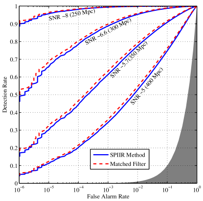
Figure 6: The receiver operating characteristics (ROC) of both the IIR filter method and the traditional matched filter method. The x-axis shows the false alarm rate, and the y-axis the detection rate. A one-to one relationship, which is the worst case scenario, is shown by the boundary of the shaded area. We show four different ROC curves, where the each curve represents the detection rate as a function of false alarm rate for waveform injected at effective distances of 250, 300, 350 and 400 $\,\mathrm{Mpc}$ (SNR $\sim$ 8, 6.6, 5.7 and 5 respectively).

V Summary and Discussion

The use of a bank of simple IIR filters for each template as opposed to the matched filter method enables us get two extra processes for a minimal additional cost. The first is that the individual IIR filter outputs can be arranged into groups, such that their total summed output is roughly independent and orthogonal to each other. This enables, with minimal extra overhead, the calculation of a $\chi^{2}$ distributed statistic, giving a secondary method of verification. We will demonstrate this in an upcoming paper. The second natural advantage of using a parallel bank of single-pole IIR filters is that they can easily be executed in parallel using multi-threaded processors, such as graphics processing units (GPUs). Indeed, a side study has shown that this is possible Liu (2011). This leads to the future possibility that a single personal computer may be able to process the detection of GWs.

A further way to reduce the computation of the IIR calculation is to split the incoming data into differently down-sampled channels. The output of each IIR filter in the bank is the correlation of a fixed frequency sinusoid and the incoming data. For the sinusoids that have frequencies $<$124$\,\mathrm{Hz}$, the incoming data need only be sampled at 256$\,\mathrm{Hz}$. The current pipeline of LLOID uses a similar multi-channel down-sampling in their detection pipeline. Their pipeline consists of the integration of the open-source real-time multimedia handling software gstreamer and the LIGO Algorithm Library (LAL) gst . This software library is an ideal platform to integrate the SPIIR method. The total computation can also be further reduced by sharing IIR filters (via interpolation) between different templates Luan (2011).

Although the design of the IIR filter so far only applies to chirping, post-Newtonian approximation inspirals, we have performed preliminary tests using more complicated combinations of single-pole IIR filters to replicate the waveform of an inspiral with spin. If the amplitude/frequency beating of a spinning inspiral waveform can be simulated by the linear addition of two different non-spinning inspirals with different masses, then it can be approximated by a linear addition of damped sinusoids. In this case, the SPIIR method can produce the SNR for the beating waveform. There is also the possibility of using higher order IIR filters, although designing the coefficients can be very difficult.

VI Conclusion

We have demonstrated that the through the use of a parallel bank of single pole IIR filters, it is possible to approximate the SNR derived from the matched filter with greater than 99% overlap. The main advantage of our SPIIR method is that it operates completely in the time domain, and in principle it has zero latency (not taking into account whitening or computational time). The SPIIR method recovers most of the injections the optimal matched filter recovers.

We foresee that the use of IIR filters for time domain filtering of Advanced LIGO will be ideal, as the waveforms will be much longer. The frequency domain matched filter will take more time to calculate GW triggers, essentially ruling out the possibility of triggering the detection the prompt optical emission related to neutron star mergers (GRBs). We have shown that the use of a parallel bank of IIR filters requires less computational cost, with minimal detection rate loss, and most importantly can be calculated in the time-domain with near zero latency.

VII Acknowledgements

We would like to thank Kipp Cannon, Drew Keppel and Chad Hanna for detailed discussion on the design and implementation of low-latency detection algorithms. This work was done in part during the LIGO Visiting Student Researcher program, which was partially funded by the 2009 UWA Research Collaboration Award. This research was supported by the Australian Research Council. SH gratefully acknowledges the support of an Australian Postgraduate Award.

Appendix A Noise Spectral Density

We use an algebraic expression for the noise spectral density of Advanced LIGO detectors defined by,

$$\begin{split}S_{h}(f)=S_{0}\left\{\left(\frac{f}{f_{0}}\right)^{-4.14}-5\left(\frac{f_{0}}{f}\right)^{2}+\right.\\ \left.111\left(\frac{1-\frac{f}{f_{0}}^{2}+0.5\frac{f}{f_{0}}^{4}}{1.+0.5\frac{f}{f_{0}}^{2}}\right)\right\};\end{split}$$ (42)

where, $f_{0}=215$Hz and $S_{0}=10^{49}$.

References

- (1) URL http://www.ligo.org.
- (2) URL http://www.virgo.infn.it/.
- Smith and for the LIGO Scientific Collaboration (2009) J. R. Smith and for the LIGO Scientific Collaboration, Classical and Quantum Gravity 26, 114013 (2009), eprint 0902.0381.
- Adv (2007) Advanced LIGO Reference Design, LIGO Tech. Rep. M060056 (2007), URL http://www.ligo.caltech.edu/docs/M/M060056-08/M060056-08.pdf.
- Abbott et al. (2009) B. P. Abbott, R. Abbott, R. Adhikari, P. Ajith, B. Allen, G. Allen, R. S. Amin, S. B. Anderson, W. G. Anderson, M. A. Arain, et al. (LIGO Scientific Collaboration), Phys. Rev. D 79, 122001 (2009).
- Fox et al. (2005) D. B. Fox, D. A. Frail, P. A. Price, S. R. Kulkarni, E. Berger, T. Piran, A. M. Soderberg, S. B. Cenko, P. B. Cameron, A. Gal-Yam, et al., Nature (London) 437, 845 (2005), eprint arXiv:astro-ph/0510110.
- Nakar (2007) E. Nakar, Phys. Rep. 442, 166 (2007), eprint arXiv:astro-ph/0701748.
- van Putten (2009) M. H. P. M. van Putten, ArXiv e-prints (2009), eprint 0905.3367.
- Zhang and Mészáros (2004) B. Zhang and P. Mészáros, International Journal of Modern Physics A 19, 2385 (2004), eprint arXiv:astro-ph/0311321.
- Wainstein and Zubakov (1962) L. A. Wainstein and V. D. Zubakov, Extraction of Signals from Noise (Prentice-Hall, 1962).
- Abbott et al. (2008) B. Abbott, R. Abbott, R. Adhikari, J. Agresti, P. Ajith, B. Allen, R. Amin, S. B. Anderson, W. G. Anderson, M. Arain, et al. (The LIGO Scientific Collaboration, http://www.ligo.org), Phys. Rev. D 77, 062002 (2008).
- Luan (2011) J. Luan, Phys. Rev. D (2011), (to be submitted).
- Buskulic et al. (2010) D. Buskulic, Virgo Collaboration, and LIGO Scientific Collaboration, Classical and Quantum Gravity 27, 194013 (2010).
- (14) URL https://www.lsc-group.phys.uwm.edu/daswg/projects/gstlal.html.
- Cannon et al. (2010) K. Cannon, A. Chapman, C. Hanna, D. Keppel, A. C. Searle, and A. J. Weinstein, Phys. Rev. D 82, 044025 (2010).
- Anderson et al. (2001) W. G. Anderson, P. R. Brady, J. D. Creighton, and É. É. Flanagan, Phys. Rev. D 63, 042003 (2001), eprint arXiv:gr-qc/0008066.
- Abbott et al. (2004) B. Abbott, R. Abbott, R. Adhikari, A. Ageev, B. Allen, R. Amin, S. B. Anderson, W. G. Anderson, M. Araya, H. Armandula, et al., Phys. Rev. D 69, 122001 (2004), eprint arXiv:gr-qc/0308069.
- Blanchet et al. (1995) L. Blanchet, T. Damour, B. R. Iyer, C. M. Will, and A. G. Wiseman, Phys. Rev. Lett. 74, 3515 (1995), eprint gr-qc/9501027.
- Blanchet et al. (1996) L. Blanchet, T. Damour, and B. R. Iyer, Phys. Rev. D 54, 1860 (1996).
- Fairhurst and Brady (2008) S. Fairhurst and P. Brady, Class. Quant. Grav. 25, 105002 (2008), eprint 0707.2410.
- Brady and Fairhurst (2008) P. R. Brady and S. Fairhurst, Classical and Quantum Gravity 25, 105002 (2008), eprint 0707.2410.
- Allen et al. (2005) B. Allen, W. G. Anderson, P. R. Brady, D. A. Brown, and J. D. E. Creighton (2005), eprint gr-qc/0509116.
- Droz et al. (1999) S. Droz, D. J. Knapp, E. Poisson, and B. J. Owen, Phys. Rev. D 59, 124016 (1999), eprint arXiv:gr-qc/9901076.
- Liu (2011) Y. Liu, J. Comput. Phys. (2011), (in preparation).