The generalized shrinkage estimator for the analysis of functional connectivity of brain signals

Abstract

We develop a new statistical method for estimating functional connectivity between neurophysiological signals represented by a multivariate time series. We use partial coherence as the measure of functional connectivity. Partial coherence identifies the frequency bands that drive the direct linear association between any pair of channels. To estimate partial coherence, one would first need an estimate of the spectral density matrix of the multivariate time series. Parametric estimators of the spectral density matrix provide good frequency resolution but could be sensitive when the parametric model is misspecified. Smoothing-based nonparametric estimators are robust to model misspecification and are consistent but may have poor frequency resolution. In this work, we develop the generalized shrinkage estimator, which is a weighted average of a parametric estimator and a nonparametric estimator. The optimal weights are frequency-specific and derived under the quadratic risk criterion so that the estimator, either the parametric estimator or the nonparametric estimator, that performs better at a particular frequency receives heavier weight. We validate the proposed estimator in a simulation study and apply it on electroencephalogram recordings from a visual-motor experiment.

TTSupported in part by the National Science Foundation (Division of Mathematical Sciences). and

1 Introduction

The goal of this paper is to estimate dependence between multi-channel electroencephalogram (EEG) signals. In the time domain, partial cross-correlation is used to measure the strength of direct linear dependence between a pair of channels. In the frequency domain, partial coherence is utilized to identify the frequency bands that drive the direct linear association. To estimate partial coherence, one first needs to estimate the spectral density matrix, which is done via a parametric method (by fitting a parametric model to the EEGs) or by some nonparametric procedure such as kernel-smoothing. Both of these procedures have their strengths and weaknesses. In this paper we develop a generalized shrinkage procedure which is a weighted average of the parametric and nonparametric estimates. The frequency-specific weights are derived data-adaptively so that the estimator (parametric versus nonparametric) that performs better at a particular frequency receives heavier weight.

To obtain a parametric estimate of the spectral density matrix, one can fit a model, such as the vector autoregressive model (VAR), which has been applied extensively in the analysis of a variety of brain signals [e.g., Goebel et al. (2003); Eichler (2005); Schlögl and Suppa (2006); Thompson and Siegle (2009)]. It is simple and can be easily applied for assessing Granger-causality and the direction of information between the signals [Kaminski and Blinowska (1991); Kaminski et al. (2001)]. Moreover, when the lag order is sufficiently large, the VAR estimates are known to be well localized in frequency. Nonparametric estimators are derived from periodogram matrices which are the data analog of the spectral density matrix. One nonparametric estimator is obtained by smoothing the periodograms across frequencies. The performance of these estimators is a function of the smoothing parameter and so these estimators may not always give well-localized estimates. However, they are asymptotically mean squared consistent and robust to model specification. In this work we develop the generalized shrinkage estimator which is a weighted average of the parametric estimator and the nonparametric estimator and thus provides a good compromise between these two estimators.

The remainder of the paper is organized as follows. In Section 2 we discuss partial coherence and the past works on shrinkage estimation. Section 3 lays out the framework for the generalized shrinkage estimator. In Section 4 we show the performance of the generalized shrinkage estimator relative to the VAR estimator, smoothed periodogram and the multitaper on a simulated data set. In Section 5 we use the generalized shrinkage estimator to analyze functional connectivity on an EEG data set. And finally, in Section 6, we summarize the conclusions of this research and briefly discuss properties of the generalized shrinkage estimator and future directions.

2 Background

Coherence, the frequency domain analog of cross-correlation, is a temporally invariant frequency-specific measure of linear association between signals. Consider a trivariate time series $(X(t),Y(t),Z(t))^{\top}$. Denote $X_{\omega}(t),Y_{\omega}(t)$ and $Z_{\omega}(t)$ to be the bandpass-filtered signals so that each of their spectra is concentrated on some narrow frequency band around $\omega$. Ombao and van Bellegem (2008) showed that coherence has an appealing interpretation of being the squared absolute cross-correlation between a pair of bandpass filtered signals, so that in this case, the coherence between $X(t)$ and $Y(t)$ at frequency $\omega$ can be interpreted as the squared cross-correlation between $X_{\omega}(t)$ and $Y_{\omega}(t)$. However, if the linear association between $X(t)$ and $Y(t)$ at frequency $\omega$ is confounded by $Z(t)$, conclusions based on the associations between $X(t)$ and $Y(t)$ may be misleading and misinterpreted because they may be related only indirectly through $Z(t)$. In other words, coherence does not model direct linear association. We can obtain a direct measure of frequency-specific linear association using partial coherence, which is interpreted as the squared cross-correlation between $X_{\omega}(t)$ and $Y_{\omega}(t)$ at frequency $\omega$ after removing the temporally invariant linear effects of $Z(t)$. To estimate partial coherence, we use a characterization that expresses partial coherence as a function of the inverse of the spectral density matrix [Dahlhaus (2000)]. In fact, this characterization was used in Eichler, Dahlhaus and Sandkühler (2003) for neural spike trains, Salvador et al. (2005) for fMRI, and Medkour, Walden and Burgess (2009) for EEG.

2.1 Characterization of partial coherence

Let ${\mathbf{X}}(t)\!=\!(X_{1}(t),\ldots,X_{P}(t))^{\top}$ be a $P$-dimensional weakly stationary zero-mean real-valued discrete time series with spectral density matrix ${\mathbf{f}}(\omega)$. The diagonal elements of ${\mathbf{f}}(\omega)$, denoted $f_{pp}(\omega)$, $p=1,\ldots,P$, are the autospectra of the $P$ channels and each of the off-diagonal elements, denoted $f_{pq}(\omega),p\neq q$, is the cross-spectrum between channels $X_{p}(t)$ and $X_{q}(t)$. Define the matrix ${\mathbf{g}}(\omega)={\mathbf{f}}^{-1}(\omega)$ whose $(p,q)$th element is denoted as $g_{pq}(\omega)$. Let ${\mathbf{h}}(\omega)$ be a diagonal matrix whose elements are $g_{pp}^{-1/2}(\omega)$. Define the matrix $\Gamma(\omega)$ to be

$$\Gamma(\omega)=-{\mathbf{h}}(\omega)\mathbf{g}(\omega){\mathbf{h}}(\omega).$$ (1)

Then the partial coherence $\rho_{pq}(\omega)$ between the $p$ and $q$th channels at frequency $\omega$ is the square of the modulus of the $(p,q)$th element of $\Gamma(\omega)$, that is, $\rho_{pq}(\omega)=|\Gamma_{pq}(\omega)|^{2}$. To estimate partial coherence, we must first estimate the spectral density matrix.

2.2 Related work on shrinkage estimation

Ledoit and Wolf (2004) proposed shrinkage estimation of the variance–covariance matrix that combines a “classical estimator” (the sample variance–covariance matrix) with a “highly-structured target.” Recently, the idea of a convex combination of a “classical estimator” with a target has been extended for estimating the spectral density matrix of a multivariate time series, which is the frequency-domain analog of the variance–covariance matrix. Böhm and von Sachs (2009) developed the shrinkage estimator for the spectral density matrix which shrinks the nonparametric estimator to the scaled identity matrix. When shrinking the nonparametric estimator toward the scaled identity matrix the resulting estimate is well conditioned. However, the off-diagonals of the estimator is shrunk to 0 and thus potentially biases the estimates of linear association toward the null. To overcome this problem, one may shrink the nonparametric estimator toward a more general shrinkage target. For factor models in economic time series, Böhm and von Sachs (2008) proposed to shrink the nonparametric estimator toward a structured model, namely, the one-factor model. Here, we extend these works by giving the shrinkage weight for any arbitrary shrinkage target.

3 The generalized shrinkage estimator

Let $\mathbf{X}_{n}(t)$, $n=1,2,\ldots,N$ and $t=1,2,\ldots,T$, be the $n$th trial of a $P$-dimensional weakly stationary zero-mean real-valued discrete time series with auto-covariance matrix $\Sigma(h)$, each of whose elements is absolutely summable. We shall assume that the trials are independent realizations from a common underlying process whose spectral properties (in particular, partial coherence) we wish to investigate. To achieve the goal of estimating partial coherence, we shall first estimate the $P\times P$ spectral density matrix defined by $\mathbf{f}(\omega)=\frac{1}{2\pi}\sum_{h\in\mathbb{Z}}\Sigma(h)\exp(-i\omega h)$. Denote the parametric estimator of $\mathbf{f}(\omega)$ to be $\widetilde{\mathbf{V}}(\omega)$ and the nonnparametric estimator to be $\widetilde{\mathbf{f}}(\omega)$. The generalized shrinkage estimator takes the weighted average of these two estimators and so takes the form

$$\mathbf{f}^{*}(\omega)=W_{T}(\omega)\widetilde{\mathbf{V}}(\omega)+\bigl{(}1-W_{T}(\omega)\bigr{)}\widetilde{\mathbf{f}}(\omega).$$ (2)

Our procedure will use the class of vector autoregressive (VAR) models whose order is selected by the Bayesian information criterion (BIC) for the parametric estimator and computes the nonparametric estimator with smoothing spans selected from a plug-in unbiased risk estimation criterion. The weight at a particular frequency is estimated data-adaptively so that a heavier weight is given to the estimator that gives a better fit at that frequency. We first describe the three components of the generalized shrinkage estimator before describing the estimation procedure.

3.1 Component 1: The parametric estimator

3.1.1 The vector autoregressive process

Here, we use the class of vector autoregressive models for obtaining a parametric estimator for the spectral density matrix. A multivariate time series $\mathbf{X}(t)$ has a VAR($K$) representation if $\mathbf{X}(t)=\sum_{k=1}^{K}\Phi_{k}\mathbf{X}(t-k)+\mathbf{Z}(t)$, where the $\Phi_{k}$’s are $P\times P$ coefficient matrices, $\mathbf{Z}(t)$ is white noise with covariance matrix $\Sigma_{Z}$, and other regularity conditions are satisfied [Brockwell and Davis (1998)]. The spectral density matrix for the VAR($K$) time series takes the form

$$\mathbf{V}(\omega) = \frac{1}{2\pi}\bigl{\{}\bigl{(}\mathbf{I}_{P}-\Phi_{1}\exp(-i\omega 1)-\cdots-\Phi_{K}\exp(-i\omega K)\bigr{)}\bigr{\}}^{-1}\times\Sigma_{Z}$$

$${}\times\bigl{\{}\bigl{(}\mathbf{I}_{P}-\Phi_{1}\exp(-i\omega 1)-\cdots-\Phi_{K}\exp(-i\omega K)\bigr{)}^{*}\bigr{\}}^{-1},$$

where $\mathbf{I}_{P}$ is the $P\times P$ identity matrix and ^∗ denotes the complex conjugate transpose. The order $K$ can be determined using some model selection criterion (such as BIC).

3.1.2 $N$-trial least squares estimation

We now describe how to obtain the least squares estimates of the coefficients of a VAR($K$) model for a multivariate time series recorded from $N$ trials. The time series for the $n$th trial is modeled as

$$\mathbf{X}_{n}(t)=\sum_{k=1}^{K}\Phi_{k}\mathbf{X}_{n}(t-k)+\mathbf{Z}_{n}(t),$$ (4)

where $\mathbf{X}_{n}(t)\!=\!(X_{1n}(t),\ldots,X_{Pn}(t))^{\top}\!$, $\mathbf{Z}_{n}(t)\!=\!(Z_{1n}(t),\ldots,Z_{Pn}(t))^{\top}\!$, $t=1,\ldots,\break T$, and $n=1,\ldots,N$. We extend the estimation for a single-trial multivariate time series in Lütkepohl (1993). Suppose we have $K$ many presample values $\mathbf{X}_{n}(-K+1),\ldots,\mathbf{X}_{n}(0)$ for each trial of this time series. For each trial $n=1,\ldots N$, define

$$\mathbf{X}_{n} = (\mathbf{X}_{n}(1),\ldots,\mathbf{X}_{n}(T))\qquad(P\times T),$$ (5)

$$\mathbf{B} = (\Phi_{1},\ldots,\Phi_{K})\qquad(P\times PK),$$ (6)

$$\mathbf{Y}_{n,t} = \pmatrix{\mathbf{X}_{n}(t)\cr\vdots\cr\mathbf{X}_{n}(t-K+1)}\qquad(PK\times 1),$$ (7)

$$\mathbf{Y}_{n} = (\mathbf{Y}_{n,0},\ldots,\mathbf{Y}_{n,T-1})\qquad(PK\times T),$$ (8)

$$\mathbf{Z}_{n} = (\mathbf{Z}_{n}(1),\ldots,\mathbf{Z}_{n}(T))\qquad(P\times T).$$ (9)

Now let $b_{k}^{\top}$ be the $k$th row of $\mathbf{B}$ and $\mathbf{X}_{n,(k)}=(\mathbf{X}_{kn}(1),\ldots,\mathbf{X}_{kn}(T))^{\top}$ and $\mathbf{Z}_{n,(k)}=(Z_{kn}(1),\ldots,Z_{kn}(T))^{\top}$. With this notation, the $n$th trial VAR($K$) model given by equation (4) can be written as $\mathbf{X}_{n,(k)}=\mathbf{Y}^{\top}_{n}b_{k}+\mathbf{Z}_{n,(k)}$. Lütkepohl (1993) gave the solution in case $N=1$ and he showed that the solution is equivalent to OLS estimation. Now for $N>1$, the setting becomes analogous to that of repeatedly measured multivariate data. From this perspective, one can see that the least squares estimator for the VAR($K$) model with $N$ trials is $\hat{b}_{k}=(\sum_{n=1}^{N}\mathbf{Y}_{n}\mathbf{Y}_{n}^{\top})^{-1}(\sum_{n=1}^{N}\mathbf{Y}_{n}\mathbf{X}_{n,(k)}).$ Suppose that $NT\gg PK$. Our estimate of $\Sigma_{Z}=\mathbb{E}(\mathbf{Z}(t)\mathbf{Z}(t)^{\top})$ is

$$\widehat{\Sigma}_{Z}=\frac{1}{NT-PK}\sum_{n=1}^{N}\{(\mathbf{X}_{n}-\widehat{\mathbf{B}}\mathbf{Y}_{n})(\mathbf{X}_{n}-\widehat{\mathbf{B}}\mathbf{Y}_{n})^{\top}\}.$$ (10)

The degrees of freedom adjustment is due to the $PK$ many coefficients in each of the $P$ equations in equation (4).

Note that in equation (4), there are $KP^{2}+P(P+1)/2$ parameters to estimate. However, it is not unusual for the number of components of the time series to be large and the number of time points per trial to be small. Therefore, it is not efficient to estimate the parameters using only a single trial. Here, we have developed a method for estimating the parameters by pooling the data over all of the trials. This is valid if one assumes that the data from each trial is a realization of a common underlying $\operatorname{VAR}(K)$ process.

The least squares estimation procedure above requires the VAR order $K$ to be known. To select the order $K$ in an $N$-trial multivariate time series framework, we use the information criterion function $\operatorname{IC}(\kappa)=\log|\widehat{\Sigma}_{Z}(\kappa)|+\operatorname{Pen}(T,N,P,\kappa)$, where $\widehat{\Sigma}_{Z}(\kappa)$ is the estimate of $\Sigma_{Z}$ obtained after fitting a VAR($\kappa$) model and $\operatorname{Pen}(T,N,P,\kappa)$ is some penalty function for complexity. Here, we use the penalty function in BIC, which is $\operatorname{Pen}(T,N,P,\kappa)=\frac{\log(NT)}{NT}\kappa P^{2}.$ The optimal order $K$ is selected so that $K=\arg\min_{\kappa}\operatorname{IC}(\kappa)$.

3.2 Component 2: The nonparametric estimator

3.2.1 The smoothed periodogram matrix

Let $\mathbf{d}_{\mathbf{X},n}(\omega)\!=\!\frac{1}{\sqrt{2\pi}}\sum_{t=1}^{T}\mathbf{X}_{n}(t)\times\exp(-i\omega t)$ be the discrete Fourier transform of $\mathbf{X}_{n}(t)$. The $n$th trial raw periodogram is defined to be $\mathbf{I}_{n}(\omega)=\frac{1}{T}\mathbf{d}_{\mathbf{X},n}(\omega)\mathbf{d}^{*}_{\mathbf{X},n}(\omega)$. Kernel smoothing is a common method for estimating the spectral density matrix. Let $w_{T}(\alpha)$ be a kernel (weight) function that has smoothing span $M_{T}$ such that, as $T\rightarrow\infty$, $M_{T}\rightarrow\infty$ but $M_{T}/T\rightarrow 0$. We compute the $n$th trial estimate of the $(j,k)$th element of $\mathbf{f}(\omega)$ with $\widetilde{f}_{n,jk}(\omega)=\int_{-\pi}^{\pi}w_{T}(\omega-\alpha)I_{n,jk}(\alpha)\,d\alpha$. Under regularity conditions [Brillinger (2001)], this estimate is an element-wise consistent estimator for $\mathbf{f}(\omega)$. The final estimate for $\mathbf{f}(\omega)$ using all of the trials is the average over the trials, namely, $\widetilde{\mathbf{f}}(\omega)=N^{-1}\sum_{n=1}^{N}\widetilde{\mathbf{f}}_{n}(\omega)$. Similarly, the elements of $\widetilde{\mathbf{f}}(\omega)$ are consistent for the elements of ${\mathbf{f}}(\omega)$. Note that in this setup, we can apply minimal smoothing per trial because the final nonparametric estimator $\widetilde{\mathbf{f}}(\omega)$ undergoes further smoothing due to the averaging across replicated trials.

3.2.2 Automatic selection of the optimal smoothing span

When $M_{T}$ is too small, the resulting estimate can capture very localized peaks but may be too erratic. Conversely, if it is too large, the resulting estimate will be very smooth but may miss vital peaks that characterize the process. Optimal smoothing spans have been studied for univariate time series. For example, the approach by Ombao et al. (2001) used the full likelihood by minimizing the gamma deviance. Here, inspired by Lee (1997) and Lee (2001), we develop an approach for span selection based on the quadratic risk function.

Define the integrated risk function for a smoothing span $h$ to be $R(h)=\int_{0}^{\pi}\mathbb{E}(\|\mathbf{f}(\omega)-\widetilde{\mathbf{f}}_{h}(\omega)\|^{2})\,d\omega$, where $\widetilde{\mathbf{f}}_{h}(\omega)$ is the periodogram matrix smoothed with a kernel having span size $h$ and $\|\cdot\|^{2}$ is the normalized Hilbert–Schmidt norm defined by $\|A\|^{2}=P^{-1}\operatorname{tr}(AA^{*})$. The goal is to pick $M_{T}$ so that $M_{T}=\arg\min_{h}R(h)$. Such an $M_{T}$ is the global optimal smoothing span. However, we cannot evaluate $R(h)$ because $\mathbf{f}(\omega)$ is unknown. An approach in the univariate time series context is to use a plug-in unbiased risk estimation (PURE) procedure by plugging in a pilot estimator $\widetilde{\mathbf{f}}_{\mathrm{pilot}}(\omega)$ for $\mathbf{f}(\omega)$, where the pilot estimator is the periodogram smoothed by a kernel with an arbitrarily picked smoothing span. This gives an asymptotically unbiased estimate of $R(h)$.

The proposed procedure for obtaining the optimal smoothing span for the $n$th trial of a multivariate time series is as follows. We combine the PURE procedure with a leave-one-out procedure. Let $\widetilde{\mathbf{f}}_{n,h}(\omega)$ be the $n$th trial periodogram smoothed with smoothing span $h$. Let $\hat{\mathbf{f}}_{(-n)}(\omega)=(N-1)^{-1}\sum_{j=1,j\neq n}^{N}\mathbf{I}_{j}(\omega)$. Since each $\mathbf{I}_{j}(\omega)$ is an approximately unbiased estimator of $\mathbf{f}(\omega)$, then $\hat{\mathbf{f}}_{(-n)}(\omega)$ is an unbiased estimate of $\mathbf{f}(\omega)$ and thus will serve as the pilot estimator. Then the $n$th trial integrated PURE is $\widehat{R}_{n}(h)=\int_{0}^{\pi}\|\hat{\mathbf{f}}_{(-n)}(\omega)-\widetilde{\mathbf{f}}_{n,h}(\omega)\|^{2}\,d\omega$. We proceed by picking the smoothing span $M^{(n)}_{T}$ for the $n$th trial so that $M^{(n)}_{T}=\arg\min_{h}\widehat{R}_{n}(h)$.

3.3 Component 3: The theoretical shrinkage weight

Ideally, the frequency-specific shrinkage weight corresponding to the parametric estimator, denoted $W_{T}(\omega)$, should be greater than 0.5 at frequencies where the parametric estimate gives a better fit than the nonparametric estimate. In fact, as we will see later, the shrinkage weight is a function of the mean squared error of each of the parametric and nonparametric estimators. We formalize this in the following discussion.

First, we introduce the notation $\mathbf{f}_{T}^{\,0}(\omega)=\mathbb{E}(\widetilde{\mathbf{f}}_{T}(\omega))$, where $\widetilde{\mathbf{f}}_{T}(\omega)$ is the smoothed periodogram. For ease, we drop the subscript $T$ in the notation. From Brillinger (2001), $\mathbf{f}^{\,0}(\omega)-\mathbf{f}(\omega)\rightarrow\mathbf{0}$ as $T\rightarrow\infty$. Here, $\mathbf{f}^{\,0}(\omega)$ will serve as the proxy for $\mathbf{f}(\omega)$ and will be utilized in deriving the weights for the generalized shrinkage estimator. Define the squared error loss function $\mathcal{L}(\mathbf{f}^{*}(\omega),\mathbf{f}^{\,0}(\omega))=\|\mathbf{f}^{*}(\omega)-\mathbf{f}^{\,0}(\omega)\|^{2},$ where the norm is the normalized Hilbert–Schmidt norm. Then the risk function is $\mathcal{R}(\mathbf{f}^{*}(\omega),\mathbf{f}^{\,0}(\omega))=\mathbb{E}(\mathcal{L}(\mathbf{f}^{*}(\omega),\mathbf{f}^{\,0}(\omega)))$. The optimal shrinkage weight $W_{T}(\omega)$ is the minimizer of the risk function. First, define

$$\alpha_{T}^{2}(\omega) = \operatorname{MSE}(\widetilde{\mathbf{V}}(\omega))=\mathbb{E}\bigl{(}\|\widetilde{\bf V}(\omega)-\mathbf{f}^{\,0}(\omega)\|^{2}\bigr{)},$$ (11)

$$\beta_{T}^{2}(\omega) = \operatorname{MSE}(\widetilde{\mathbf{f}}(\omega))=\mathbb{E}\bigl{(}\|\widetilde{\mathbf{f}}(\omega)-\mathbf{f}^{\,0}(\omega)\|^{2}\bigr{)}$$ (12)

and

$$\delta_{T}^{2}(\omega)=\mathbb{E}\bigl{(}\|\widetilde{\bf V}(\omega)-\widetilde{\mathbf{f}}(\omega)\|^{2}\bigr{)}.$$ (13)

Then it can be easily shown the optimal shrinkage weight is

$$W_{T}(\omega)=\frac{\beta_{T}^{2}(\omega)-0.5(\alpha_{T}^{2}(\omega)+\beta_{T}^{2}(\omega)-\delta_{T}^{2}(\omega))}{\delta_{T}^{2}(\omega)}.$$ (14)

This result generalizes that given by both Böhm and von Sachs (2008), whose shrinkage target was that of a one-factor model, and Böhm and von Sachs (2009), whose shrinkage target was the scaled identity matrix.

Upon inspection of the optimal shrinkage weight equa-tion (14), one can obtain insight that the generalized shrinkage estimator behaves analogous to the Bayes estimators, where the prior estimator is given by the parametric estimator and the data-driven estimator is given by the nonparametric estimator. Note that the behavior of the shrinkage weight is a function of the relative performance of each of the parametric and nonparametric estimators. In particular, if the parametric estimator models the spectral density matrix well so that $\alpha_{T}^{2}(\omega)\rightarrow 0$ at a rate much faster than $\beta_{T}^{2}(\omega)\rightarrow 0$, then the shrinkage weight will shift toward the parametric estimator; otherwise, the shrinkage weight will shift toward the nonparametric estimator. The second term of the numerator of equation (14) corrects for the correlation between the parametric estimator and the nonparametric estimator. Empirical Bayes estimators use the data to construct the prior estimator. Our approach is analagous in the sense that we use the same data to construct the parametric and nonparametric estimators, and so the second term takes into account that the two estimators are highly likely to be correlated. Back to equation (14), we see that the denominator makes the generalized shrinkage estimator robust to the misspecification of the parametric estimator. The denominator is the squared distance between the parametric and nonparametric estimators. So if the parametric and nonparametric estimators are vastly different from each other, then the denominator of the weight will be large, and so the weight will be larger for the nonparametric estimator.

3.4 Constructing the generalized shrinkage estimator

The parametric and nonparametric components of the generalized shrinkage estimator can be obtained using standard procedures. To estimate the shrinkage weight, we need to construct an estimate of each of $\alpha^{2}_{T}(\omega)$ and $\beta^{2}_{T}(\omega)$, and $\delta^{2}_{T}(\omega)$.

Each of $\alpha^{2}_{T}(\omega)$ and $\beta_{T}^{2}(\omega)$ is the expected distance from their respective estimator with $\mathbf{f}^{\,0}(\omega)$, and so we need to provide an estimate of $\mathbf{f}^{\,0}(\omega)$. An asymptotically unbiased estimator of $\mathbf{f}^{\,0}(\omega)$ is the average of the periodograms: $\hat{\mathbf{f}}^{\,0}(\omega)=N^{-1}\sum_{n=1}^{N}\mathbf{I}_{n}(\omega)$. Consider $\beta_{T}^{2}(\omega)$. Since $\widetilde{\mathbf{f}}(\omega)$ is an unbiased estimator of $\mathbf{f}^{\,0}(\omega)$ by construction, then $\beta_{T}^{2}(\omega)$ is the sum over the variances of each of the elements of $\widetilde{\mathbf{f}}(\omega)$. Assuming that each element of $\hat{\mathbf{f}}^{\,0}(\omega)$ varies slowly over frequency, our proposed estimator is a type of sample variance, that is, we look at the window of size $C_{T}$ around $\widetilde{\mathbf{f}}(\omega)$ for each $\omega$:

$$\hat{\beta}^{2}_{T}(\omega)=C_{T}^{-1}\sum_{k=-(C_{T}-1)/2}^{(C_{T}-1)/2}\|\widetilde{\mathbf{f}}(\omega)-\hat{\mathbf{f}}^{\,0}(\omega+\omega_{k})\|^{2}.$$ (15)

Our simulation studies indicate the choice of this procedure is robust over a wide choice for $C_{T}$. We estimate $\alpha_{T}^{2}(\omega)$ using a type of plug-in estimator smoothed over frequencies:

$$\hat{\alpha}^{2}_{T}(\omega)=C_{T}^{-1}\sum_{k=-(C_{T}-1)/2}^{(C_{T}-1)/2}\|\widetilde{\mathbf{V}}(\omega)-\hat{\mathbf{f}}^{\,0}(\omega+\omega_{k})\|^{2}.$$ (16)

Our proposed estimator for $\delta_{T}^{2}(\omega)$ is constructed in a similar manner:

$$\hat{\delta}^{2}_{T}(\omega) = \frac{1}{2}\Biggl{[}C_{T}^{-1}\sum_{k=-(C_{T}-1)/2}^{(C_{T}-1)/2}\bigl{(}\|\widetilde{\mathbf{f}}(\omega+\omega_{k})-\widetilde{\mathbf{V}}(\omega)\|^{2}$$

$${}\hskip 91.0pt+\|\widetilde{\mathbf{V}}(\omega+\omega_{k})-\widetilde{\mathbf{f}}(\omega)\|^{2}\bigr{)}\Biggr{]}.$$

Then we can obtain a plug-in estimate of the optimal shrinkage weight using

$$\widehat{W}_{T}(\omega)=\frac{\hat{\beta}^{2}_{T}(\omega)-0.5(\hat{\alpha}_{T}^{2}(\omega)+\hat{\beta}_{T}^{2}(\omega)-\hat{\delta}_{T}^{2}(\omega))}{\hat{\delta}^{2}_{T}(\omega)}.$$ (18)

Note that due to estimation error in obtaining $\hat{\alpha}_{T}^{2}(\omega)$, $\hat{\beta}_{T}^{2}(\omega)$ and $\hat{\delta}_{T}^{2}(\omega)$, it is possible for our estimate of the shrinkage weight to fall outside the interval $[0,1]$. If this occurs, we truncate the estimated weight to 0 or 1. Finally, we plug in the estimated weight to obtain an estimate of the generalized shrinkage estimator:

$$\hat{\mathbf{f}}^{*}(\omega)=\widehat{W}_{T}(\omega)\widetilde{\mathbf{V}}(\omega)+\bigl{(}1-\widehat{W}_{T}(\omega)\bigr{)}\widetilde{\mathbf{f}}(\omega).$$ (19)

4 Simulation study

We now compare the performance of the generalized shrinkage estimator against competitors which are, namely, the VAR estimator whose order is selected using the BIC criteria, the smoothed periodogram and the multitaper [Percival and Walden (1993)]. The VAR estimator was estimated as described in Section 3.1. The smoothed periodogram, as described in Section 3.2, is obtained using the Hann kernel whose smoothing span is objectively determined by the quadratic risk criterion described in Section 3.2.2. The multitaper estimator was obtained by averaging the per-trial multitaper estimates, which is similar to how we obtained the smoothed periodogram estimator. The optimal number of tapers was also objectively determined using a PURE procedure similar to that described in Section 3.2. The estimators are compared using the mean squared error (MSE).

The true underlying process was a sum of a VAR($5$) process and a first-order vector moving average (VMA) process. The two processes were generated independently so that the underlying spectral density matrix is the sum of that of the VAR and the VMA. The vector time series had $P=12$ dimensions, $N=120$ trials, and $T=256$ time points. The values of the parameters are given in the Appendix.

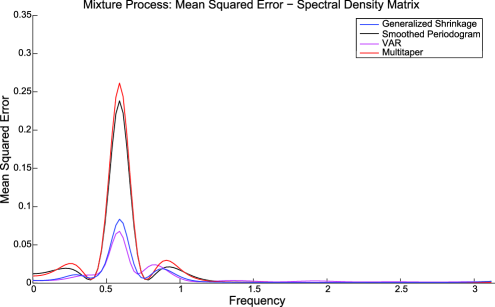
(a)

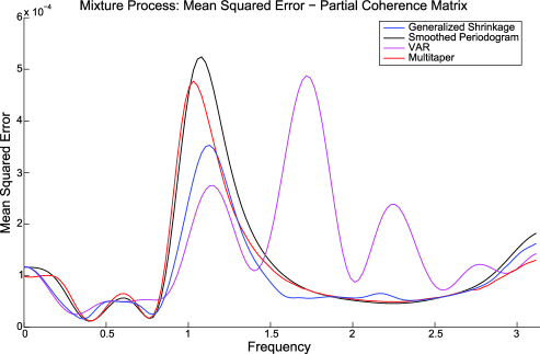
(b)

Figure 1: Mean squared error estimated via Monte Carlo for the simulation. (a) Frequency-specific mean squared error of each estimate of the spectral density matrix. (b) Frequency-specific mean squared error of each estimate of the partial coherence matrix.

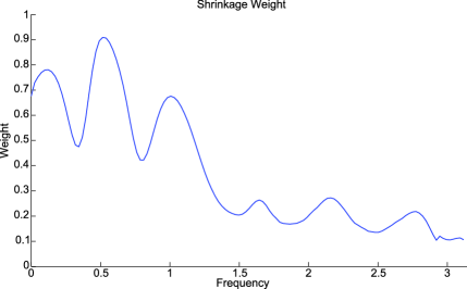
Figure 2: Shrinkage weight for the generalized shinkage estimator estimated via Monte Carlo for the simulation.

The results of the simulation study are shown in Figure 1. Under this setting, it is obvious that the VAR parametric estimator was incorrectly specified. However, as just noted earlier, a VAR can capture the peaks in the spectral density matrix. Note that while the VAR estimator is the best estimator of the spectral density matrix in the sense that it accurately captured the peaks in the autospectra, it was not necessarily the best estimator of partial coherence (because the latter is a highly nonlinear function of the former). This can be seen in the high frequencies as shown in Figure 1. In other words, the best estimator of the spectral density matrix is not necessarily the best estimator for partial coherence. The nonparametric estimators performed poorly relative to the parametric VAR estimator in estimating the spectral density matrix because each oversmoothed the peaks in the autospectra. The generalized shrinkage estimator performed well in estimating both the spectral density matrix and partial coherence. It is clear that the generalized shrinkage estimator borrowed strength from the parametric VAR estimator to better capture the peaks in the autospectra so that it estimated the spectral density matrix much better than the nonparametric estimators. This can be seen by the shrinkage weight, as shown in Figure 2. The shrinkage weight is near 1.0 at frequencies near the location of the peaks of the autospectra.

5 Functional connectivity for EEG

The study of functional connectivity of brain signals is the investigation of the dependencies between brain signals that have been measured from spatially separated regions of the brain [Friston et al. (1993)]. We investigated the dependency structure in the EEG signals between certain regions and how it differs across experimental conditions in a visual-motor task.

5.1 Data description and preprocessing

The EEG data were recorded from the scalp using a 64-channel EEG system (EMS, Biomed, Korneuburg, Germany). The electrodes were applied to the scalp using the standard International 10–20 system with a reference electrode on the nose-tip. The EEG signals were recorded at 512 samples/second/channel and filtered using a high-pass filter of 0.02 Hz and a low-pass filter of 100 Hz.

Participants of the study were required to make quick displacements of a hand-held joystick from a central position either to the right or to the left from center as instructed by a visual cue. The visual cue randomly selected the movement per trial. From a standard montage of 64 scalp electrodes, our neuroscientist collaborator selected a subset of $P=12$ channels that were presumed, based on published studies, to be recording the relevant neural processes for these visual-motor actions [Marconi et al. (2001); Bédard and Sanes (2009)]. These electrode sites include the fronto-central leads (FC) to measure activity related to premotor processing, the central leads (C) to measure activity related to motor performance, and the parietal (P) and occipital (O) leads to measure activity related to visual-motor transformations. We did not add more electrodes in the analysis because this will present unnecessary computing and modeling complications, which we will later discuss. The relative locations of these 12 electrode sites are shown in Figure 3.

The methods that we have developed in this work have been for single-subject analyses, and so here, we show results for only one subject. We analyze the first 0.5 seconds from stimulus onset of the EEG signals, yielding a multivariate time series having length $T=256$ per trial, and there were $N_{\mathrm{L}}=118$ and $N_{\mathrm{R}}=138$ trials for the leftward and rightward movements respectively. For the analysis, we removed the linear and quadratic trends from the subject’s EEGs. The EEGs were further filtered using a $4$th-order low-pass Butterworth filter with stopband at 50 Hz and then standardized to have unit variance. Figure 4 illustrates time plots of the $P=12$ filtered and detrended EEG signals obtained from a representative participant during leftward and rightward joystick movements.

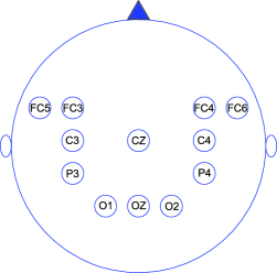
Figure 3: Relative placement of the twelve EEG channels preselected for the analysis. These channels were presumed to be recording the relevant neural processes for the visual-motor task in the experiment.

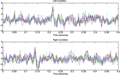
Figure 4: Representative 12-channel filtered and detrended EEG recorded from one trial for each of the left and right conditions.

5.2 Details on the statistical procedure

Our aim in this work was two-fold: first, to estimate the strength of functional connectivity as measured by partial coherence, and second, to identify which connections differentiate between the “left” and the “right” trials. The parametric component was computed using a VAR(19) model where the order was selected using the BIC criterion and the parameters were estimated using the $N$-trials least squares procedure. The nonparametric component was obtained using the Hann kernel with smoothing span automatically selected by our procedure. The mean smoothing span selected for the trials for the “left” conditions was 23.37 with standard deviation 7.74 and for the “right” conditions 22.04 with standard deviation 7.75. The estimated partial coherences are shown in Figure 5. To perform a frequency-band analysis of functional connectivity, we computed the partial coherences averaged over the frequencies in the band of interest. The partial coherences for each of the alpha band (8–12 Hz) and beta band (18–30 Hz) for each of the “left” and “right” conditions are shown in Figure 6.

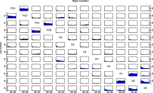
Figure 5: Estimated partial coherence for all pairs of the twelve channels in the analysis for the “right” condition (upper triangle) and the “left” condition (lower triangle).

To test for differences in strength of connectivity over a frequency band, we normalized the partial coherence estimates using the Fisher’s $Z$-transform. We used the jackknife to estimate the standard error of the estimated partial coherences over the bands. This was done by, after leaving out one trial, estimating partial coherence via the generalized shrinkage estimator of the spectral density matrix and then using Fisher’s $Z$-transform to normalize these jackknifed partial coherence estimates. This allowed us to obtain a jackknife sample of size $N_{\mathrm{L}}$ estimates of partial coherence for each of the frequency bands for the “left” condition and a jackknife sample of size $N_{\mathrm{R}}$ estimates of partial coherence for each of the frequency bands for the “right” condition. The point estimates for each of the conditions as well as their standard errors, both estimated using a sample size $N_{\mathrm{L}}$ or $N_{\mathrm{R}}$, allowed us to create $t$-statistics to test for differences via a two-sample $t$-test across conditions. These $t$-statistics are shown in Figure 7. Note that for each frequency band, we performed $12\cdot(12-1)/2=66$ tests, so that in all we are performing 132 tests. To correct for multiple comparisons, we performed our tests controlling for FDR at $0.05$. The null hypotheses of no difference across conditions that were rejected are marked with an asterisk in Figure 7.

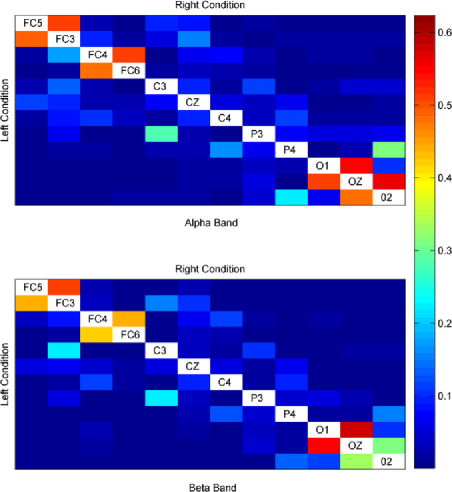
Figure 6: Relative strength of functional connectivity measured by partial coherence at the alpha and beta frequency bands for the “right” condition (upper triangle) and “left” condition (lower triangle).

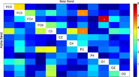
Figure 7: The absolute value of the $t$-statistics for testing for differences between “left” and “right” conditions. The $t$-statistics marked with an asterisk (*) were declared significant after adjusting their $p$-values at FDR level of 0.05.

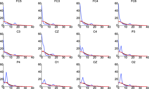
(a)

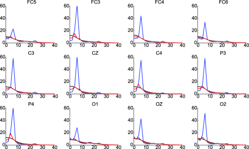
(b)

Figure 8: Estimated autospectra for each of the two conditions. Shown here are the three estimators: the VAR(19) (blue), the smoothed periodogram (black), and the generalized shrinkage (red). (a) Estimated autospectra for the “left” condition. (b) Estimated autospectra for the “right” condition.

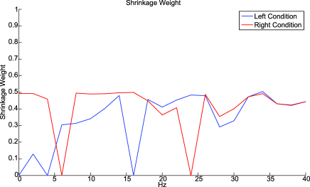
Figure 9: Estimated shrinkage weight.

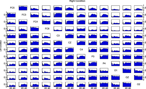
Figure 10: Estimated coherence for all pairs of the twelve channels in the analysis for the “right” condition (upper triangle) and the “left” condition (lower triangle).

5.3 Results

On the estimates of the autospectra. The estimated power spectral densities for each channel are shown in Figure 8(a) and (b), and the estimated shrinkage weight is shown in Figure 9. For the “left” condition, the VAR estimator picks up a peak in the autospectra at the very low frequencies, and then a smaller peak around 16 Hz. At these frequencies, the generalized shrinkage estimator disagreed with the VAR estimator, and, in fact, the shrinkage weight was truncated to $0.0$ at these frequencies. For the “right” condition, again the VAR estimator picks up two peaks, one around 6 Hz and the other around $24$ Hz, and the smoothed periodogram oversmoothed these peaks. The estimate of the shrinkage weight was not truncated at 0.0 at 4 Hz, and so the estimates given by the generalized shrinkage estimator are showing a slight peak. The shrinkage weight was much less than $0.5$, and so the smoothed periodogram was favored. This implies that the VAR model may not be an adequate model.

On the estimates of partial coherence. Figure 10 shows the estimated coherence for all pairs. Recall that coherence is the frequency domain analog of squared cross-correlation. Coherence among the fronto-central leads and among the occipital leads are strong, in fact, near 1.0 at some frequencies. The coherence between the occipital leads and the fronto-central leads is smaller. Since coherence captures both direct and indirect connectivity, then we can see that the occipital leads are somehow connected with the fronto-central leads. Partial coherence captures only the direct connectivity by removing the effects of the other leads in the analysis. In Figure 5 we see that the strong direct connections are among the fronto-central leads and the occipital leads. Moreover, the connections between the fronto-central leads and the occipital leads are much weaker after partialization, suggesting that the connection between these regions is more likely to be indirect.

On comparing connectivity between left vs right conditions. When testing for differences of the “left” and “right” connections as shown in Figure 7, some of the differences in strength of connections were deemed statistically significant. However, upon closer inspection, many of these differences may be considered to be irrelevant because the estimated strength of connection is very weak. For instance, the difference in strength in the O1–FC4 connection in the beta band had the largest $t$-statistic and was considered statistically significant, and yet, the estimated partial coherence values for this connection are $0.0225$ and $0.0116$ for the “left” and “right” conditions, respectively. Though this is nearly a $2$-fold increase in strength of connection, these squared correlation values are small and so the connection may not be relevant to the visual-motor task. Among those pairs where the estimated partial coherence is larger than 0.05 for at least one of the conditions, differences between conditions were significant for the following pairs: C3–FC5, P3–C3 and O2–OZ in the alpha band and FC3–FC5, FC3–FC4, C3–FC3 and P3–C3 in the beta band.

Of these differences, the only connection where it is stronger in the “left” condition is the P3–C3 connection; for the other differences, the “right” condition yielded stronger connections. An analysis by Böhm et al. (2010) concluded that the coherence between C3 and FC3 was the most discriminating feature between the two conditions using frequency-domain characteristics of the EEG signals. Our jackknife procedure is consistent with this finding and even provides additional information, namely, that a measure of the direct connection between C3 and FC3 may be used to distinguish between “left” and “right” conditions.

On the limitations of EEG. While EEGs have excellent temporal resolution, they are not highly localized in space. Nevertheless, they remain highly utilized in many studies because they have excellent temporal resolution and thus can be used to probe into brain processes that occur at the millisecond level. Moreover, they are relatively inexpensive to collect, noninvasive and highly portable, and thus have the high potential for brain–computer interface applications.

On the limitations of partial coherence. Partial coherence is a tool for investigating second-order dependencies for a given set of channels. Partial coherence measures only the strength of direct dependencies and does not give information of the direction of the dependencies, which can be captured using other metrics of association [e.g., Kaminski et al. (2001)]. Moreover, certain regions may be strongly connected but in a nonlinear manner, and if this is the case, we would have missed this in the present analysis because partial coherence measures only linear associations between the signals and the spectral density matrix captures only second-order dependencies. One can investigate nonlinear and higher order dependencies in multivariate time series using metrics such as mutual information.

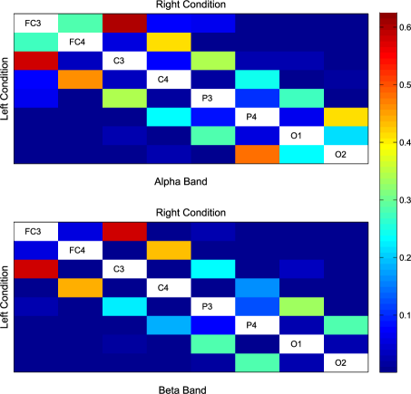
Figure 11: Relative strength of functional connectivity measured by partial coherence at the alpha and beta frequency bands for the “right” condition (upper triangle) and “left” condition (lower triangle) when $P=8$ channels are analyzed.

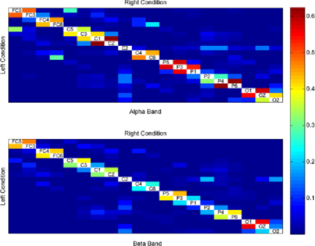
Figure 12: Relative strength of functional connectivity measured by partial coherence at the alpha and beta frequency bands for the “right” condition (upper triangle) and “left” condition (lower triangle) when $P=20$ channels are analyzed.

On the importance of the selection of the channels. Since partial coherence measures direct dependencies, the choice of the channels to include in the analysis is important. We illustrate this by showing how the estimates of the partial coherence are affected when signals from more and less channels are included in the analysis.

We first see the effects if channels were removed. Figure 11 shows the estimates of partial coherence for $P=8$. Compare the estimates of partial coherence between FC3 and FC4 in the alpha band as shown in Figure 11 with that shown in Figure 6. The partial coherence is larger for the case $P=8$ because the signals from the FC5 and FC6 channels were excluded. Then in the 12-channel analysis, when computing partial coherence between FC3 and FC4, the effects of FC5 were removed from FC4, and since FC5 is highly conditionally dependent with FC3 (as shown in Figure 6), this dampened the partial coherence between FC3 and FC4. In fact, partial coherence estimates are larger for the $P=8$ analysis, and this is due to the exclusion of certain channels.

Consider now the situation when more channels are included. Figure 12 shows the estimates of partial coherence for $P=20$. Here, partial coherence estimates are smaller due to the inclusion of certain channels. Let us look at the partial coherence between P3 and C3 in the alpha band. Now for $P=20$, partial coherence between P3 and C3 removes the effects of each of C5 and P5. By removing the effects of P5 from C3, one is also removing the effects of P3 because P3 and P5 are highly conditionally dependent, and, similarly, by removing the effects of C5 from P3, one is removing the effects of C3 because C3 and C5 are highly conditionally dependent. Thus, the partial coherence between P3 and C3 is lower when C5 and P5 are included in the analysis.

This motivates the importance of the choice of channels in the analysis. As we have just shown, including or excluding channels can have an effect on the analysis. However, one should not include everything in the analysis for two reasons. First, there is the problem of high-dimensionality, which can lead to problems in inference because there are more connectivity measures to estimate. Second, we note that many of these (neighboring) channels are highly correlated with each other, which then introduces redundant information. So if all channels were included in the analysis, we expect that many of the partial coherence estimates will be dampened down to 0.

6 Discussion

Our main contribution for spectral analysis in multivariate time series is a new estimator for estimating the spectral density matrix. Our approach simply takes the weighted average of two known estimators, namely, a parametric and nonparametric estimator. We derived the weights using a multivariate mean squared error criterion. We have made further developments in shrinkage estimation for the spectral density matrix by giving freedom in the choice of the shrinkage target and by giving the appropriate shrinkage weight for this choice of the shrinkage target. Our shrinkage target in this work is the spectral density matrix for a VAR model. We have proposed a method to take advantage of the trials of an experiment for estimating the parameters of the VAR model. Our nonparametric estimator is the classical smoothed periodogram. We have proposed a method to take advantage of the trials of an experiment to select the optimal smoothing span of the smoothing kernel. We then outlined a simple method for estimating the optimal shrinkage weight to construct the generalized shrinkage estimator and then evaluated its performance on simulated data sets before using it to analyze functional connectivity in an EEG data set.

The performance of the generalized shrinkage estimator is a function of the performance of each of the parametric and nonparametric components. In fact, it can be shown that the risk for the generalized shrinkage estimator is a weighted average of the risk of each of the two components less a correction term for the distance between the two components. If the true spectral density matrix can be well approximated by that given by a VAR model, then an estimator based on the VAR model alone will outperform the generalized shrinkage estimator. However, one can never truly know how well the VAR model approximates the true spectral density matrix. Our generalized shrinkage estimator first fits the VAR model, and then adjusts this fit with the nonparametric smoothed periodogram. The optimal shrinkage weight is picked by minimizing the risk over all $P$ dimensions of the multivariate time series simultaneously. This can be problematic if there is a wide range of dynamics across the dimensions of the multivariate time series. For instance, if the autospectra for all but one dimension were flat and there is a sharp peak in that one dimension, then though the VAR estimator will capture that peak and the smoothed periodogram oversmooths that peak, the generalized shrinkage estimator will not give the VAR estimator a lot of weight just to capture that one peak.

There is still a great amount of work to be done with the generalized shrinkage estimator. It remains to show the large-sample behavior of the generalized shrinkage estimator for estimating the spectral density matrix. Large-sample results were given for the shrinkage estimators described by Böhm and von Sachs (2008) and Böhm and von Sachs (2009). However, their work constrained the class of shrinkage targets; Böhm and von Sachs (2009) used the scaled identity matrix as the shrinkage target as a way of regularizing the smoothed periodogram and the shrinkage target used by Böhm and von Sachs (2008) was specifically the one-factor model. In both works they were able to show consistency of their shrinkage estimator. In this work, though we used the VAR model as the shrinkage target, when we developed the generalized shrinkage estimator we have refrained from imposing conditions on the shrinkage target, and, in fact, our results on the optimal shrinkage weight remains valid for any shrinkage target. Recall that the number of parameters in a $\operatorname{VAR}(K)$ model is of the order $KP^{2}$. It may be the case that imposing more constraints to decrease the parameter space of the VAR model or considering other shrinkage targets with a low-dimensional parameter space will improve the performance of the generalized shrinkage estimator. In the future, we would like to investigate the large-sample performance of the generalized shrinkage estimator when constraints are imposed on the shrinkage target.

We do not have asymptotic distributions for the estimated partial coherence in a frequency band via generalized shrinkage. Test statistics in the literature have been for partial noncorrelation between two signals so that the test for zero partial coherence is for all frequencies. Parametric tests for this null hypothesis have been provided by, for example, Dahlhaus, Eichler and Sandkühler (1997) and Dahlhaus (2000). Nonparametric tests, on the other hand, are difficult to construct; to create a boostrap distribution, for instance, one would have to somehow preserve the correlation structure that exists in the other frequency bands that are not of interest. One approach is to shuffle the data across trials in order to completely destroy the correlation structure, but tests on partial coherence over a frequency band using this approach will have a larger Type I error than advertised. However, one can take advantage of the multiple trials in the experiment and the multiple experimental conditions to investigate the differences in connectivity across the experimental conditions using nonparametric tests, as we have done here using the jackknife.

Appendix: Simulation settings

The coefficient matrix for the VMA process is as follows. First, let

$$\mathbf{\theta}_{1}=\pmatrix{0&0.20&0.15&0.15&0&-0.15\cr 0.20&0&-0.20&0&0&0\cr-0.15&0.20&0&0&0&0\cr 0&0&0&0&0.20&0.15\cr 0&0&0&0.20&0&-0.20\cr 0&0&0&-0.15&0.20&0}.$$

Then the coefficient matrix is

$$\mathbf{\Theta}_{1}=\pmatrix{\theta_{1}&\mathbf{0}_{6}\cr\mathbf{0}_{6}&\theta_{1}}.$$

The coefficient matrices for the VAR process are as follows. Let

$$\phi_{1}=(0.75,0.75,0.75).$$

Then the two coefficient matrices are

$$\mathbf{\Phi}_{1} = \operatorname{diag}(\phi_{1},\phi_{1},\phi_{1},\phi_{1}),\qquad\mathbf{\Phi}_{2}=-0.20\cdot\mathbf{I}_{12},\qquad\mathbf{\Phi}_{3}=\mathbf{0}_{12},$$

$$\mathbf{\Phi}_{4} = -0.15\cdot\mathbf{I}_{12}\quad\mbox{and}\quad\mathbf{\Phi}_{5}=-0.05\cdot\mathbf{I}_{12}.$$

The noise process $\mathbf{Z}(t)$ is a zero-mean 12-dimensional Gaussian process with variance–covariance matrix $\mathbf{I}_{12}$. A realization $\mathbf{X}(t)$ of the mixture process takes the form $\mathbf{X}(t)=0.65\cdot\mathbf{X}_{\mathrm{MA}}(t)+0.35\cdot\mathbf{X}_{\mathrm{AR}}(t)$, where $\mathbf{X}_{\mathrm{MA}}(t)$ is a VMA and $\mathbf{X}_{\mathrm{AR}}(t)$ is a VAR, and the two are independent. Because the two processes are independent, then the spectral density matrix of the mixture process is the weighted sum of the spectral density matrix of the VMA process and the spectral density matrix of the VAR process.

References

- Bédard and Sanes (2009) Bédard, P. and Sanes, J. (2009). Gaze and hand position effects on finger-movement-related human brain activation. J. Neurophysiol. 101 834–842.
- Böhm et al. (2010) Böhm, H., Ombao, H., von Sachs, R. and Sanes, J. (2010). Classification of multivariate non-stationary signals: The SLEX-shrinkage approach. J. Statist. Plann. Inference 3754–3763. \MR2674163
- Böhm and von Sachs (2008) Böhm, H. and von Sachs, R. (2008). Structural shrinkage of nonparametric spectral estimators for multivariate time series. Electron. J. Statist. 2 696–721. \MR2430251
- Böhm and von Sachs (2009) Böhm, H. and von Sachs, R. (2009). Shrinkage estimation in the frequency domain of multivariate time series. J. Multivariate Anal. 100 913–935. \MR2498723
- Brillinger (2001) Brillinger, D. (2001). Time Series: Data Analysis and Theory. SIAM, Philadelphia, PA. \MR1853554
- Brockwell and Davis (1998) Brockwell, P. and Davis, R. (1998). Time Series: Theory and Methods. Springer, New York. \MR0868859
- Dahlhaus (2000) Dahlhaus, R. (2000). Graphical interaction models for multivariate time series. Metrika 51 157–172. \MR1790930
- Dahlhaus, Eichler and Sandkühler (1997) Dahlhaus, R., Eichler, M. and Sandkühler, J. (1997). Identification of synaptic connections in neural ensembles by graphical models. J. Neurosci. Methods 77 93–107.
- Eichler (2005) Eichler, M. (2005). A graphical approach for evaluating effective connectivity in neural systems. Philos. Trans. Roy. Soc. B 360 953–967.
- Eichler, Dahlhaus and Sandkühler (2003) Eichler, M., Dahlhaus, R. and Sandkühler, J. (2003). Partial correlation analysis for the identification of synaptic connections. Biol. Cybernet. 89 289–302.
- Friston et al. (1993) Friston, K., Frith, C., Liddle, P. and Frackowiak, R. (1993). Functional connectivity: The principal-component analysis of large (pet) data sets. Journal of Cerebral Blood Flow and Metabolism 13 5–14.
- Goebel et al. (2003) Goebel, R., Roebroecka, A., Kim, D.-S. and Formisano, E. (2003). Investigating directed cortical interactions in time-resolved fmri data using vector autoregressive modeling and granger causality mapping. Magnetic Resonance Imaging 21 1251–1261.
- Kaminski and Blinowska (1991) Kaminski, M. and Blinowska, K. (1991). A new method of the description of the information flow in the brain structures. Biol. Cybernet. 65 203–210.
- Kaminski et al. (2001) Kaminski, M., Ding, M., Truccolo, W. and Bressler, S. (2001). Evaluating causal relations in neural systems: Granger causality, directed transfer function and statistical assessment of significance. Biol. Cybernet. 85 145–157.
- Ledoit and Wolf (2004) Ledoit, O. and Wolf, M. (2004). A well-conditioned estimator for large-dimensional covariance matrices. J. Multivariate Anal. 88 365–411. \MR2026339
- Lee (1997) Lee, T. (1997). A simple span selector for periodogram smoothing. Biometrika 84 965–969. \MR1625012
- Lee (2001) Lee, T. (2001). A stabilized bandwidth selection method for kernel smoothing of the periodogram. Signal Processing 81 419–430.
- Lütkepohl (1993) Lütkepohl, H. (1993). Introduction to Multiple Time Series Analysis. Springer, Berlin. \MR1239442
- Marconi et al. (2001) Marconi, B., Genovesio, A., Battaglia-Mayer, A., Ferraina, S., Squatrito, S., Molinari, M., Lacquaniti, F. and Caminiti, R. (2001). Eye-hand coordination during reaching. i. Anatomical relationships between parietal and frontal cortex. Cerebral Cortex 11 513–527.
- Medkour, Walden and Burgess (2009) Medkour, T., Walden, A. and Burgess, A. (2009). Graphical modelling for brain connectivity via partial coherence. J. Neurosci. Methods 180 374–383.
- Ombao et al. (2001) Ombao, H., Raz, J., Strawderman, R. and von Sachs, R. (2001). A simple generalised crossvalidation method of span selection for periodogram smoothing. Biometrika 88 1186–1192. \MR1872229
- Ombao and van Bellegem (2008) Ombao, H. and van Bellegem, S. (2008). Coherence analysis: A linear filtering point of view. IEEE Trans. Signal Process. 56 2259–2266. \MR2516630
- Percival and Walden (1993) Percival, D. B. and Walden, A. T. (1993). Spectral Analysis for Physical Applications: Multitaper and Conventional Univariate Techniques. Cambridge Univ. Press, Cambridge. \MR1297763
- Salvador et al. (2005) Salvador, R., Suckling, J., Schwarzbauer, C. and Bullmore, E. (2005). Undirected graphs of frequency-dependent functional connectivity in whole-brain networks. Philos. Trans. Roy. Soc. B 360 937–946.
- Schlögl and Suppa (2006) Schlögl, A. and Suppa, G. (2006). Analyzing event-related eeg data with multivariate autoregressive parameters. Progress in Brain Research 159 135–147.
- Thompson and Siegle (2009) Thompson, W. and Siegle, G. (2009). A stimulus-locked vector autoregressive model for slow event-related fmri designs. NeuroImage 46 739–748.