Lattice QCD and Hydro/Cascade Model of Heavy Ion Collisions

Abstract

We report here on a recent lattice study of the QCD transition region at finite temperature and zero chemical potential using domain wall fermions (DWF). We also present a parameterization of the QCD equation of state obtained from lattice QCD that is suitable for use in hydrodynamics studies of heavy ion collisions. Finally, we show preliminary results from a multi-stage hydrodynamics/hadron cascade model of a heavy ion collision, in an attempt to understand how well the experimental data (e.g. particle spectra, elliptic flow, and HBT radii) can constrain the inputs (e.g. initial temperature, freezeout temperature, shear viscosity, equation of state) of the theoretical model.

1 Introduction

The aim of the various high energy heavy ion collision (HIC) programs at experimental facilities such as RHIC, SPS, LHC, and FAIR is to study the properties of nuclear matter under the extreme conditions of high energy and high density. In particular, at sufficiently high energy density, it is predicted that normal hadronic matter will undergo a transition into a wholly new state of matter, the quark-gluon plasma (QGP) [1, 2], where the constituent quarks and gluons will no longer be confined within hadronic states and chiral symmetry is restored.

In principle, the properties of the QGP can be calculated directly from the underlying theory, Quantum Chromodynamics (QCD). In practice, ab initio calculations via lattice QCD require very large-scale computing resources. It is only recently that high-precision lattice QCD results[3, 4, 5, 6, 7, 8] have become available that have the potential to quantatively constrain models of heavy ion collisions. In Sec. 2 we discuss a lattice calculation[9] that uses the domain wall fermion method[10] to calculate the crossover temperature of QCD at zero chemical potential. In section 3 we present a parameterization of a high-precision lattice calculation of the QCD Equation of State (EoS) that is useful for modeling heavy ion collisions.

In addition to theoretical calculations of the QGP, a robust understanding of the dynamics of a heavy ion collision is needed in order to translate experimental results into constraints on the physical properties of hot QCD matter. Several approaches, such as Boltzman transport, hydrodynamics, and hadronic cascade [11, 12, 13, 14] have been used to model heavy ion collisions. However, the relevant physics changes so drastically over the lifetime of a HIC that it is difficult to capture all the aspects of a collision with a single model. In Sec. 4 we present preliminary results on a multi-stage model of a HIC that incorporates Glauber initial conditions with pre-equilibrium flow, 2-d viscous hydrodynamics, Cooper-Frye freezeout, and a hadronic cascade.

2 QCD Transition using domain wall fermions

The location of the QCD crossover has been a subject of much debate in the past several years [4, 5, 6]. Because of computational expediency, many of these high-precision studies have been done using the staggered fermion formulation. Although computationally inexpensive, staggered fermions have the known flaw that they only preserve a $U(1)$ subgroup of the full $SU(N_{f})$ chiral symmetry at finite lattice spacing. This manifests itself in large lattice artifacts in certain quantities, e.g. non-degeneracy in the pion spectrum. Domain Wall Fermions (DWF) preserve the full $SU(N_{f})$ chiral symmetry at finite lattice spacing [10]. Thus, a DWF study at finite temperature is useful to test the robustness of the recent staggered studies of $T_{c}$ and helps us to better understand the role of chiral symmetry in the QCD crossover.

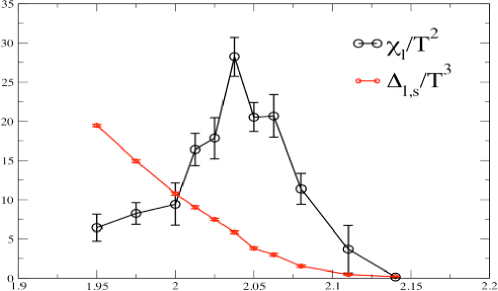
Figure 1: The disconnected chiral susceptibility, $\chi_{l}/T^{2}$ and the subtracted chiral condensate, $\Delta_{l,s}/T^{3}$. as a function of the bare lattice coupling $\beta=6/g_{0}^{2}$. The peak in the disconnected chiral susceptibility corresponds to $T\approx 170~{}\textrm{MeV}$.

In our DWF calculation [9], we perform simulations at 11 different temperatures in the range $120~{}\textrm{MeV}<T<220~{}\textrm{MeV}$ at zero chemical potential. We use a temporal lattice size of $N_{t}=8$, which is related to the temperature via $T=1/(N_{t}a)$. These temperatures correspond to lattice spacings in the range $0.11~{}\textrm{fm}<a<0.21~{}\textrm{fm}$.

Various quantities are used to locate the chiral-symmetry restoring and deconfinement transitions. For the chiral transition, we use the subtracted chiral condensate,

$$\frac{\Delta_{l,s}(T)}{T^{3}}=\frac{\left<\bar{\psi}_{l}\psi_{l}\right>-\frac{m_{l}}{m_{s}}\left<\bar{\psi_{s}}\psi_{s}\right>}{T^{3}},$$ (1)

where the subscripts $l,s$ denote the light and strange quarks, respectively. In the phase where chiral symmetry is restored ($T>T_{c}$), we expect $\Delta_{l,s}(T)$ to vanish, while for $T<T_{c}$, it is non-zero. In addition to the chiral condensate, we also calculate the disconnected chiral susceptibility,

$$\frac{\chi_{l}}{T^{2}}=VT^{3}\left(\left<\left(\bar{\psi_{l}}\psi_{l}\right)^{2}\right>-\left<\bar{\psi_{l}}\psi_{l}\right>^{2}\right).$$ (2)

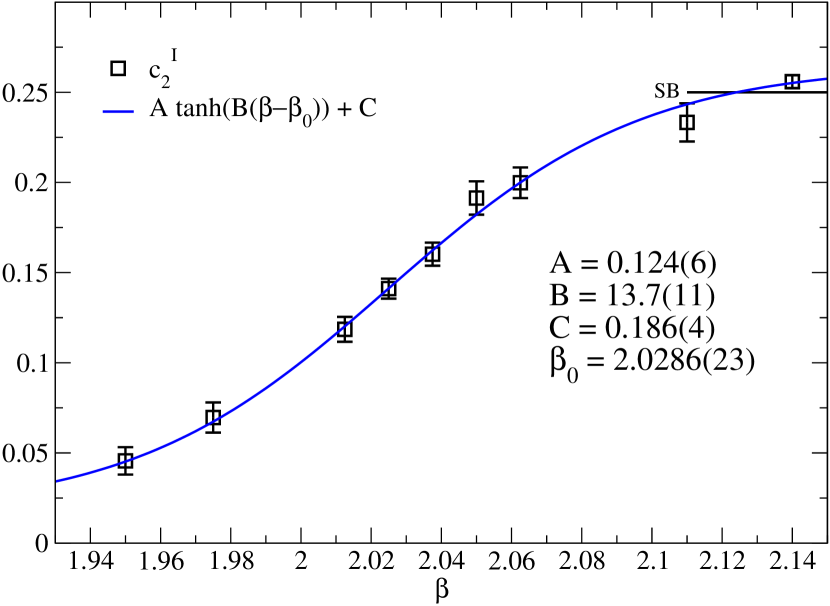
Figure 2: The isospin susceptibility, $c_{2}^{I}$ versus bare coupling $\beta=6/g_{0}^{2}$.

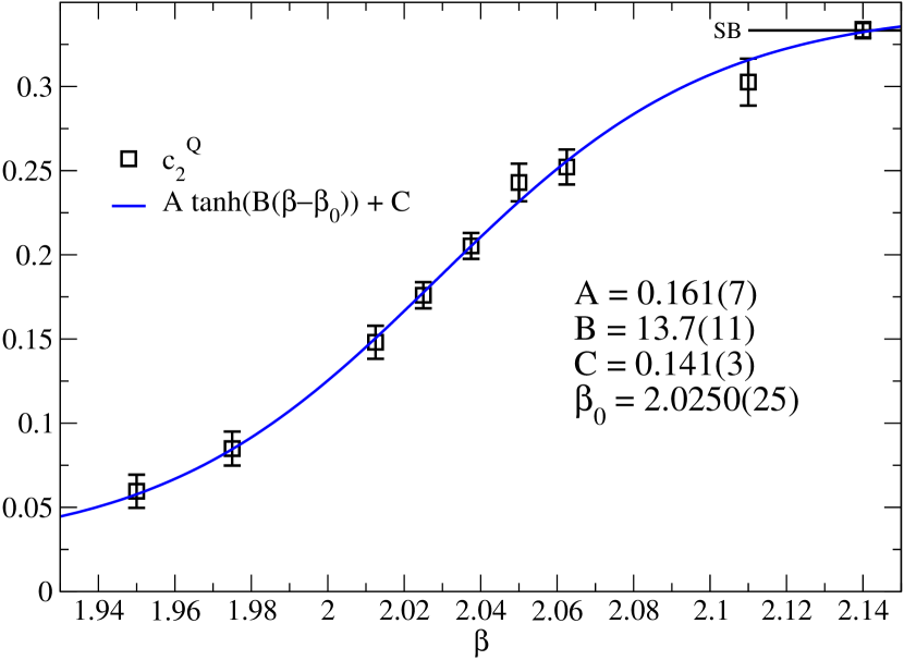
Figure 3: The electric charge susceptibility, $c_{2}^{Q}$ versus bare coupling $\beta=6/g_{0}^{2}$.

This quantity should exhibit a peak at $T=T_{c}$. Fig. 1 shows both $\frac{\Delta_{l,s}}{T^{3}}$ and $\frac{\chi_{l}}{T^{2}}$. As can be seen, the disconnected chiral susceptibility has a clear peak near $\beta=6/g_{0}^{2}=2.03$, where $g_{0}$ is the bare coupling on the lattice. This corresponds to $T\approx 170$ MeV.

For the deconfinement transition, we calculate the electric charge susceptibility ($c_{2}^{Q}$) and the isospin susceptibility ($c_{2}^{I}$):

$$\frac{c_{2}^{X}}{T^{2}}=\frac{1}{2}\frac{1}{VT^{3}}\frac{\partial^{2}\ln Z}{\partial(\mu_{X}/T)^{2}}|_{\mu_{X}=0};~{}\textrm{X = Q, I},$$ (3)

where $\mu_{Q}$ and $\mu_{I}$ are the electric charge and isospin chemical potentials and $\ln Z$ is the QCD partition function. As can be seen in Figs. 3 and 3, these deconfinement observables show a rapid rise in the same general region as those observables related to chiral symmetry.

Although the chiral susceptibility has a clear peak near $T\approx 170~{}\textrm{MeV}$ and the electric charge and isospin susceptibilities imply $T_{c}$ in the same region, our calculation still suffers from significant uncertainties. The spatial volume used is quite small, from $V=(1.7~{}\textrm{fm})^{3}$ up to $V=(3.1~{}\textrm{fm})^{3}$, so our result may be polluted with uncontrolled finite-volume effects. In addition, the light quark masses are not physical, but correspond to $m_{\pi}=300$ MeV near the susceptibility peak. Furthermore, the simulations are not done on a line of constant quark mass, so that $m_{\pi}$ is effectively much heavier at low temperatures than at high temperatures. These effects introduce significant uncertainty into our estimate of $T_{c}$, so we are only able to quote a wide range of possible values: $150~{}\textrm{MeV}<T<190~{}\textrm{MeV}$. Unfortunately, this does not do much to discriminate between the results of recent lattice calculations, but we hope to reduce these uncertainties in future calculations.

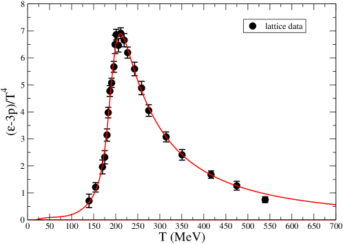
Figure 4: Lattice QCD results of the interaction measure $(\epsilon-3p)/T^{4}$ with corresponding fit to the parameterization $I(T)=(1/I_{low}(T)+1/I_{high}(T))^{-1}$.

3 Parameterization of the lattice QCD equation of state

There have been several attempts to parameterize the lattice results for the QCD equation of state (EoS) in terms of a continuous function that can be conveniently input into hydrodynamic models. Our parameterization reproduces the expected asymptotic behavior of the QCD equation of state in the limits $T\rightarrow 0$ and $T\rightarrow\infty$, smoothly joining them together in the intermediate regime near the QCD crossover.

In lattice calculations, the interaction measure (I(T) = $\epsilon-3p$) is the thermodynamic quantity that is naturally calculated, from which all other thermodynamics quantities such as the pressure $p$, energy density $\epsilon$, entropy density $s$, and speed of sound $c_{s}$ can be derived. Thus, it is sufficient to parameterize the interaction measure.

In the high temperature limit, the interaction measure is expected to have the form [15, 16]:

$$\frac{I_{high}(T)}{T^{4}}=\frac{\alpha_{1}}{T^{4}}+\frac{\alpha_{2}}{T^{4}}.$$ (4)

The lattice QCD data agrees well with this expected behavior. At low temperatures, QCD can be described as a gas of mesons and baryons. A widely-used approximation is to assume that this gas is non-interacting. This is called the Hadron Resonance Gas (HRG) model [17].

The existing lattice results give an interaction measure that tends to be lower than that given by the HRG model at low temperatures. Thus, in our parameterization, deviations from the HRG model at low temperature are included in order to accurately fit the lattice data:

$$\frac{I_{low}(T)}{T^{4}}=\frac{I_{HRG}(T)}{T^{4}}\left(\alpha_{3}+\left(\frac{T}{\alpha_{4}}\right)^{\alpha_{5}}\right).$$ (5)

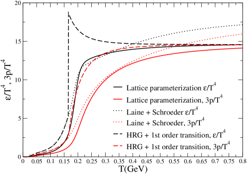
Figure 5: Comparison of the energy density, $\epsilon$ and three times the pressure, 3p, for our lattice parameterization, the EoS from Laine and Schroeder [18], and the Hadron Resonance Gas Model with a 1st order transition.

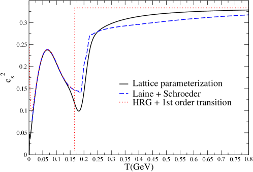
Figure 6: Comparison of the speed of sound squared, $c_{s}^{2}$, for our lattice parameterization, the EoS from Laine and Schroeder [18], and the Hadron Resonance Gas Model with a 1st order transition.

The low and high temperature parameterizations are combined via:

$$I(T)=\left(\frac{1}{I_{low}(T)}+\frac{1}{I_{high}(T)}\right)^{-1}$$ (6)

and the parameters ($\alpha_{1}\cdots\alpha_{5}$) can be extracted through a fit to the lattice data. Note that fixing $\alpha_{3}=1$ is also an option, if one wants to force the parameterization onto the HRG result as $T\rightarrow 0$.

Table 1 tabulates the fit parameters ($\alpha_{1}\cdots\alpha_{5}$) from a fit to the lattice EoS for the p4 action at $N_{t}=8$ [8]. Fig. 4 shows the result of this parameterization plotted along with the actual lattice data. Fig. 5 shows a comparison of this lattice parameterization with two other forms for the equation of state often used in hydrodynamic modeling - a form proposed by Laine and Schroeder [18], and one where the HRG EoS at low temperature is joined to an ideal gas at high temperature with a first-order phase transition at $T_{c}=165$ MeV. Figure 6 shows the same comparison for the speed of sound squared, $c_{s}^{2}$.

$\alpha_{1}$	$\alpha_{2}$	$\alpha_{3}$	$\alpha_{4}$	$\alpha_{5}$
0.26867	0.00345	0.50120	0.18529	15.17516

Table 1: Fit parameters for $I(T)$.

4 Hydro+Cascade Model

We introduce a multi-stage model where a heavy ion collision is modeled from the first moment of collision until the final state hadrons are effectively free-streaming to the particle detectors. In constructing this model, we wish to systematically test the effect of varying various model inputs and to see which set of parameters give the best agreement with experimental results. Among the things that we wish to test are: the nature of the initial conditions, the inclusion of pre-equilibirum flow, the initial temperature $T_{i}$, the shear viscosity $\eta$, the freezeout temperature $T_{f}$, and the equation of state.

4.1 Initial Conditions

For initial conditions, we use an optical Glauber model [19, 20], where the initial energy density is proportional to the number of participant nuclei, $N_{part}$ or the number of binary collisions, $N_{coll}$. The magnitude of the energy density is chosen so that the maximum energy density $\epsilon_{max}$ corresponds to some initial temperature, $T_{i}$. The impact parameter, $b$ can be directly varied to obtain different centralities.

A commonly used assumption is that the initial flow velocities vanishes, neglecting the fact that flow velocities may develop in the first $\tau\approx 1$ fm/c, before hydrodynamic evolution is applicable [21]. Recently, it has been found that neglecting initial flow velocities might have significant effects on collective observables, particularly those related to the source size [22, 23]. Therefore, we allow the modification of our initial conditions to account for possible pre-thermalization flow.

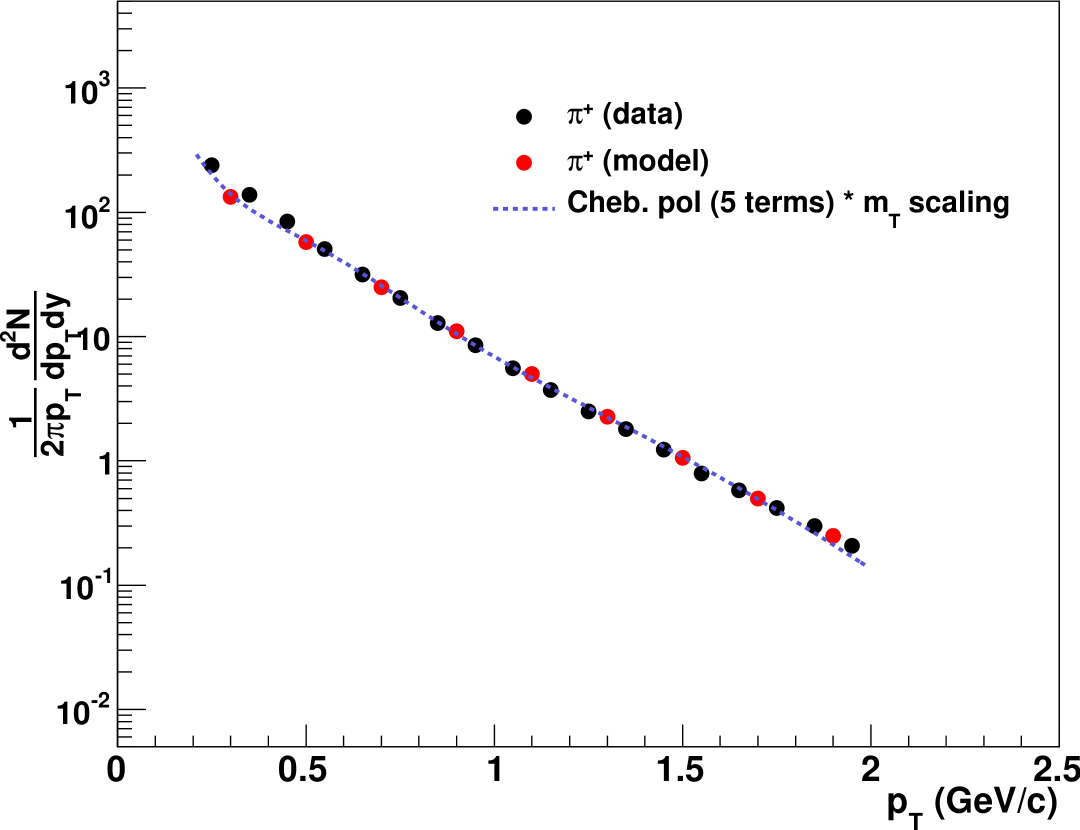
Figure 7: $\pi^{+}$ invariant yield. Experimental data from PHENIX results in the $10-15\%$ centrality bin [24]. Model results obtained with impact parameter $b=4.4\textrm{fm}$, $T_{i}=300\textrm{MeV}$, $T_{f}=150\textrm{MeV}$, without initial flow and using the ”lattice-inspired” EoS.

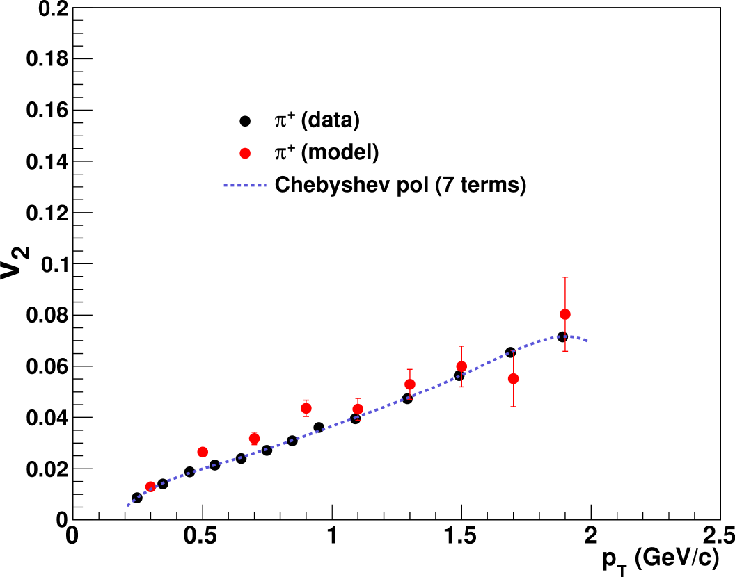
Figure 8: $\pi^{+}$ elliptic flow ($v_{2}$). Experimental data from PHENIX results in the $0-10\%$ centrality bin [25]. Model results obtained with impact parameter $b=4.4\textrm{fm}$, $T_{i}=300\textrm{MeV}$, $T_{f}=150\textrm{MeV}$, without initial flow and using the ”lattice-inspired” EoS.

4.2 Viscous Hydrodynamics

Because the relativistic generalizations of the Navier-Stokes equation are acausal, it is not entirely clear how to formulate relativistic dissipative hydrodynamics. One attempt is the Israel-Stewart formalism [26], where a relaxation time is introduced for every transport coefficient. However, there is still ambiguity as to which higher order terms to include. In the case of vanishing bulk viscosity, however, it has been shown [27] that the most general form includes five additional terms, $\tau_{\Pi},\kappa,\lambda_{1},\lambda_{2},\lambda_{3}$, where $\kappa=0$ in flat space-time. This formulation was implemented by Romatshke [28], and is the one that we utilize.

Romatschke’s code [28] is two-dimensional, where the bulk viscosity ($\zeta$) implicitly vanishes, but the shear viscosity ($\eta$) can be non-zero. For the relaxation times, we set $\tau_{\Pi}=6\eta/sT$, $\lambda_{1}=0$, $\lambda_{2}=-2\eta/\tau_{\Pi}$, $\lambda_{3}=0$, which are valid choices for a weakly-coupled plasma. The start time for the hydrodynamics evolution is taken to be $\tau_{0}=1fm/c$, with the initial conditions discussed above.

For the equation of state, we plan to test four different variations: 1) A HRG EoS for $T<T_{c}$ with a first order transition, 2) the ”Laine-Schroder” EoS [18] used in [28], 3) a parameterization of the lattice QCD EoS discussed in Sec. 3, and 4) the parmeterization of the lattice QCD EoS with $\alpha_{3}=1$ so that it is smoothly joined to the HRG EoS at low temperatures. A comparison of the first three of these can be seen in Figs. 5 and 6.

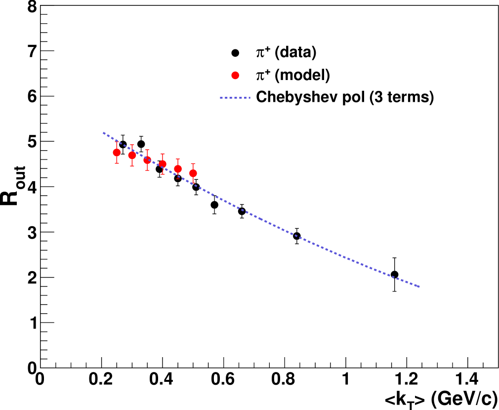
Figure 9: $\pi^{+}$ $R_{out}$. Experimental data from PHENIX results in the $0-30\%$ centrality bin [29]. Model results obtained with impact parameter $b=4.4\textrm{fm}$, $T_{i}=300\textrm{MeV}$, $T_{f}=150\textrm{MeV}$, without initial flow and using the EoS from Laine and Schroeder.

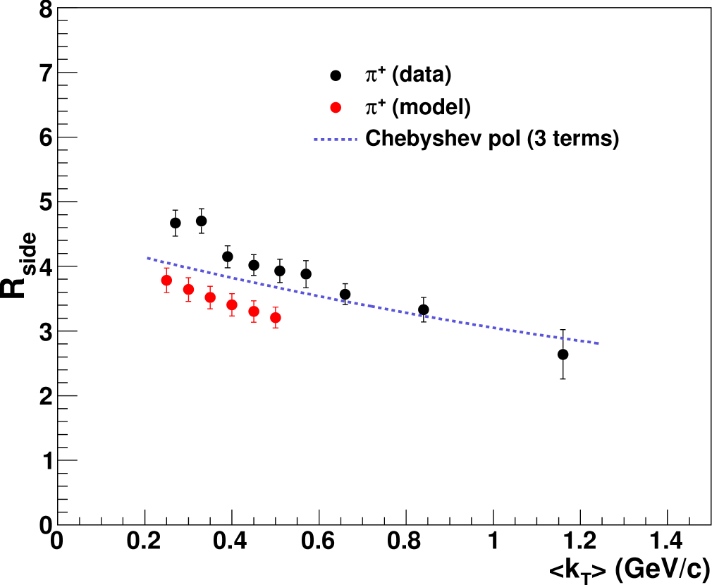
Figure 10: $\pi^{+}$ $R_{side}$. Experimental data from PHENIX results in the $0-30\%$ centrality bin [29]. Model results obtained with impact parameter $b=4.4\textrm{fm}$, $T_{i}=300\textrm{MeV}$, $T_{f}=150\textrm{MeV}$, without initial flow and using the EoS from Laine and Schroeder.

4.3 Cooper-Frye Freezeout

In modeling the freezeout of hadrons from the QGP, we use sudden freezeout and the Cooper- Frye prescription. In this method, the hadrons are frozen out on a hypersurface in $(x,y,z,t)$ of constant temperature $T=T_{f}$, or equivalently constant energy density. This freezeout temperature can be varied to study the effects of early or late freezeout. The single particle spectrum using the Cooper-Frye method is given by:

$$E\frac{dN}{d^{3}\bf{p}}=\frac{d}{(2\pi)^{3}}\int p_{\mu}d\Sigma^{\mu}f(x^{\mu},p^{\mu}),$$ (7)

where $d$ is the degeneracy factor, $d\Sigma^{\mu}$ represents the normal to the freezeout hypersurface, and $f(x^{\mu},p^{\mu})$ is the phase space density with non-equilibrium corrections [30].

Because the hydrodynamic evolution occurs only in two spatial dimensions, we assume boost- invariance along the longitudinal direction to produce the full freezeout spectrum for the particles.

4.4 Hadron Cascade

After freezeout, one must take into account final state interactions and feed-down decays in order to extract the final particle spectra. In order to do this, we take the particles produced at freezeout and evolve them through a hadronic cascade. The code that we choose is the Ultrarelativistic Quantum Molecular Dynamics (UrQMD) code [13, 14], a microscopic transport code that explicitly takes into account particle decays and hadron-hadron collisions.

4.5 Preliminary Results

We have preliminary results for several model runs corresponding to Au+Au collisions at $\sqrt{s}=200$ GeV per nucleon pair. The parameters that we have used are summarized in Tab. 2. However, we have not yet explored all possible variations of the model inputs. The impact parameter of $b=4.4$ fm. was chosen to match as closely as possible to the mid-centraility bins for PHENIX results.

To match to experimental data, we concentrate on three classes of observables: 1) the invariant yield $(1/2\pi p_{T})(dN/dp_{T}dy)$ at mid-rapidity, 2) the elliptic flow $v_{2}$, and 3) the HBT radii, $R_{out},R_{side}$, and $R_{long}$. To determine the degree of agreement with experimental, we perform a joint fit of both the model and experimental results to a common smoothing function. For $v_{2}$ and the HBT radii, the smoothing function we use is a set of orthonormal polynomials, the Chebyshev polynomials. For the invariant yield, we found that the product of Chebyshev polynomials with $\exp\left(-m_{T}/T\right)$, where $m_{T}=m^{2}+p_{T}^{2}$, produced the best fits. Fig. 8 shows the fit of the invariant yield for $\pi^{+}$ with one set of model parameters. Fig. 8 shows the fit for $v_{2}$ and Figs. 10 and 10 show HBT radii.

For each set of model parameters, the joint fit with the experimental data produces a value of $\chi^{2}$, which is a loose measure of the difference between the model and experiment. Figs. 12 and 12 show the $\chi^{2}$ distributions for $\pi^{+}$ for the invariant yield and $v_{2}$ as a function of $T_{i}$ and $\eta/s$.

As this is a work in progress, we plan to perform a systematic exploration of the model parameter space, and perform these joint fits with a larger set of experimental results. We intend to understand how sensitive the final results are to the various model inputs, and which model inputs give the best match to experimental results for various systems, energies, and centralities.

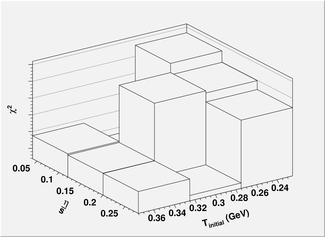
Figure 11: $\chi^{2}$ distribution for model/data fits in the $\pi^{+}$ invariant yield as a function of $T_{i}$ and $\eta/s$.

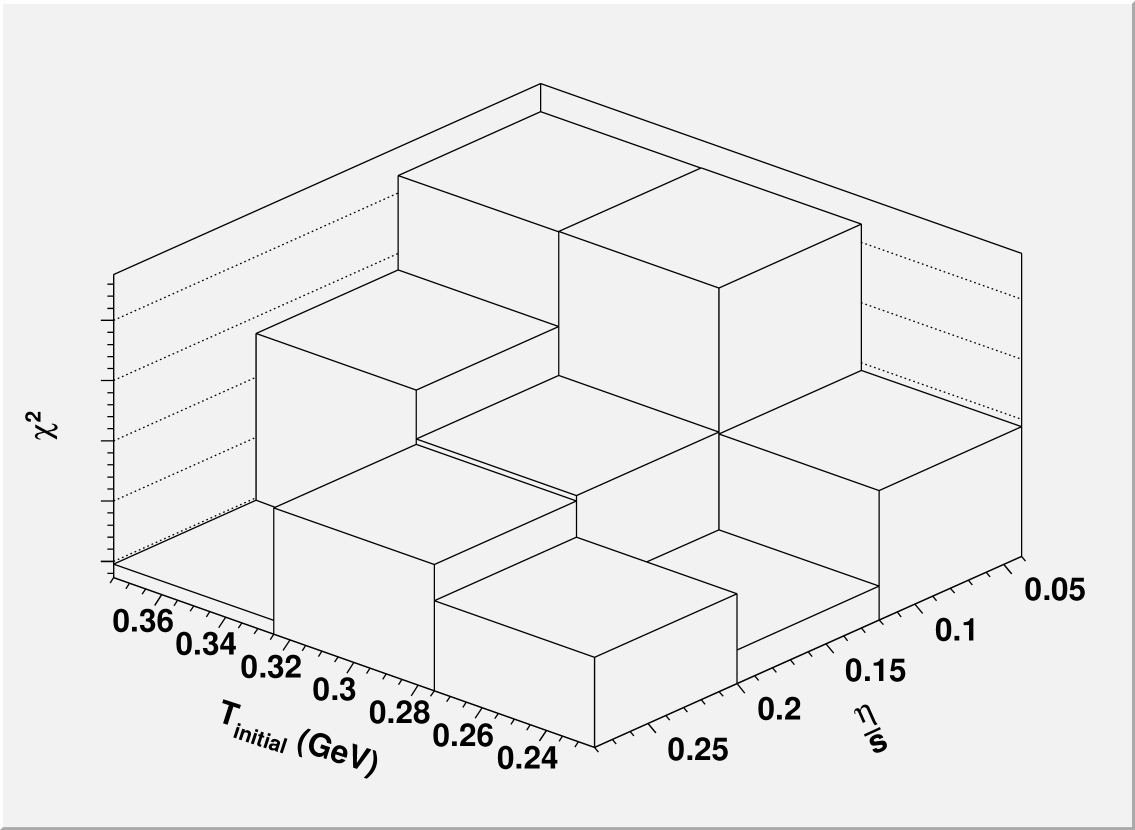
Figure 12: $\chi^{2}$ distribution for model/data fits in $\pi^{+}$ $v_{2}$ as a function of $T_{i}$ and $\eta/s$.

b (fm)	$N_{part}$	$T_{i}$ (MeV)	$\eta/s$	$T_{f}$ (MeV)	Initial Flow	EoS
4.4	270	250, 300, 350	0.08, 0.16, 0.24	150	yes, no	Laine & Schroder

Table 2: A summation of the model parameters that have been explored so far for Au+Au collisons at $\sqrt{s}=200$ GeV per nucleon pair.

References

- [1] Collins J C and Perry M J 1975 Phys. Rev. Lett. 34 1353
- [2] Shuryak E V 1980 Phys. Rept. 61 71–158
- [3] Aoki Y, Fodor Z, Katz S D and Szabo K K 2006 JHEP 01 089 (Preprint hep-lat/0510084)
- [4] Aoki Y, Z, Katz S D and Szabo K K 2006 Phys. Lett. B643 46–54 (Preprint hep-lat/0609068)
- [5] Aoki Y et al. 2009 JHEP 06 088 (Preprint 0903.4155)
- [6] Cheng M et al. 2006 Phys. Rev. D74 054507 (Preprint hep-lat/0608013)
- [7] Cheng M et al. 2008 Phys. Rev. D77 014511 (Preprint 0710.0354)
- [8] Bazavov A et al. 2009 Phys. Rev. D80 014504 (Preprint 0903.4379)
- [9] Cheng M et al. 2010 Phys. Rev. D81 054510 (Preprint 0911.3450)
- [10] Kaplan D B 1992 Phys. Lett. B288 342–347 (Preprint hep-lat/9206013)
- [11] Molnar D and Gyulassy M 2002 Nucl. Phys. A697 495–520 (Preprint nucl-th/0104073)
- [12] Teaney D, Lauret J and Shuryak E V 2001 Phys. Rev. Lett. 86 4783–4786 (Preprint nucl-th/0011058)
- [13] Bleicher M et al. 1999 J. Phys. G25 1859–1896 (Preprint hep-ph/9909407)
- [14] Bass S A et al. 1998 Prog. Part. Nucl. Phys. 41 255–369 (Preprint nucl-th/9803035)
- [15] Pisarski R D 2007 Prog. Theor. Phys. Suppl. 168 276–284 (Preprint hep-ph/0612191)
- [16] Megias E, Ruiz Arriola E and Salcedo L L 2007 Phys. Rev. D75 105019 (Preprint hep-ph/0702055)
- [17] Hagedorn R 1965 Nuovo Cim. Suppl. 3 147–186
- [18] Laine M and Schroder Y 2006 Phys. Rev. D73 085009 (Preprint hep-ph/0603048)
- [19] Glauber R J 1955 Phys. Rev. 100 242–248
- [20] Miller M L, Reygers K, Sanders S J and Steinberg P 2007 Ann. Rev. Nucl. Part. Sci. 57 205–243 (Preprint nucl-ex/0701025)
- [21] Huovinen P and Ruuskanen P V 2006 Ann. Rev. Nucl. Part. Sci. 56 163–206 (Preprint nucl-th/0605008)
- [22] Pratt S 2009 Phys. Rev. Lett. 102 232301 (Preprint 0811.3363)
- [23] Vredevoogd J and Pratt S 2009 Phys. Rev. C79 044915 (Preprint 0810.4325)
- [24] Adler S S et al. (PHENIX) 2004 Phys. Rev. C69 034909 (Preprint nucl-ex/0307022)
- [25] Afanasiev S et al. (PHENIX) 2009 Phys. Rev. C80 024909 (Preprint 0905.1070)
- [26] Israel W and Stewart J M 1979 Ann. Phys. 118 341–372
- [27] Baier R, Romatschke P, Son D T, Starinets A O and Stephanov M A 2008 JHEP 04 100 (Preprint 0712.2451)
- [28] Luzum M and Romatschke P 2008 Phys. Rev. C78 034915 (Preprint 0804.4015)
- [29] Adler S S et al. (PHENIX) 2004 Phys. Rev. Lett. 93 152302 (Preprint nucl-ex/0401003)
- [30] Pratt S and Torrieri G 2010 (Preprint 1003.0413)