Glauber Modeling in High Energy
Nuclear Collisions

Abstract

This is a review of the theoretical background, experimental techniques, and phenomenology of what is called the “Glauber Model” in relativistic heavy ion physics. This model is used to calculate “geometric” quantities, which are typically expressed as impact parameter ($b$), number of participating nucleons ($N_{\mathrm{part}}$) and number of binary nucleon-nucleon collisions ($N_{\mathrm{coll}}$). A brief history of the original Glauber model is presented, with emphasis on its development into the purely classical, geometric picture that is used for present-day data analyses. Distinctions are made between the “optical limit” and Monte Carlo approaches, which are often used interchangably but have some essential differences in particular contexts. The methods used by the four RHIC experiments are compared and contrasted, although the end results are reassuringly similar for the various geometric observables. Finally, several important RHIC measurements are highlighted that rely on geometric quantities, estimated from Glauber calculations, to draw insight from experimental observables. The status and future of Glauber modeling in the next generation of heavy ion physics studies is briefly discussed.

1 Introduction

Ultra-relativistic collisions of nuclei produce the highest multiplicities of outgoing particles of all subatomic systems known in the laboratory. Thousands of particles are created when two nuclei collide head-on, generating event images of dramatic complexity compared with proton-proton collisions. The latter is a natural point of comparison, as nuclei are themselves made up of nucleons, i.e. protons and neutrons. Thus, it is natural to ask just how many nucleons are involved in any particular collision or, more reasonably, in a sample of selected collisions. It is also an interesting to consider other ways to characterize the overlapping nuclei, e.g. their shape.

While this problem would seem intractable, with the femtoscopic length scales involved precluding direct observation of the impact parameter ($b$) or number of participating nucleons ($N_{\mathrm{part}}$) or binary nucleon-nucleon collisions ($N_{\mathrm{coll}}$), theoretical techniques have been developed to allow estimation of these quantities from experimental data. These techniques, which consider the multiple- scattering of nucleons in nuclear targets, are generally referred to as “Glauber Models” after Roy Glauber. Glauber pioneered the use of quantum mechanical scattering theory for composite systems, describing non trivial effects discovered in cross sections for proton-nucleus (p+A) and nucleus-nucleus (A+B) collisions at low energies.

Over the years, a variety of methods were developed for calculating geometric quantities relevant for p+A and A+B collisions [1, 2, 3]. Moreover, a wide variety of experimental methods were tried to connect distributions of measured quantities to the distributions of geometric quantities. This review is an attempt to explain how the RHIC experiments grappled with this problem, and largely succeeded, both because of good-sense experimental and theoretical thinking.

Heavy ion physics entered a new era with the turn-on of the RHIC collider in 2000 [4]. Previous generations of heavy ion experiments searching for the Quark Gluon Plasma (QGP) had focused on particular signatures suggested by theory. From this strategy, experiments generally measured observables in different regions of phase space, or focused on particular particle types. RHIC experiments were designed in a comprehensive way, with certain regions of phase space being covered by multiple experiments. This allowed systematic cross checks of various measurements between experiments, increasing the credibility of the separate results [5, 6, 7, 8].

Among the most fundamental observables shared between the experiments were those relating to the geometry of the collision. Identical Zero-Degree Calorimeters [9] were installed in all experiments to estimate the number of spectator nucleons, and all experiments had coverage for multiplicities and energy measurements over a wide angular range. This allowed a set of systematic studies of centrality in d+Au and A+A collisions, providing one of the first truly extensive datasets all of which characterized by geometric quantities.

This review will cover the basic information a newcomer to the field should know to understand how centrality is estimated by the experiments, and how this is related to nucleus-nucleus collisions. Section 2 will discuss the history of the Glauber model by reference to the theoretical description of nucleus-nucleus collisions. Section 3 will discuss how experiments measure centrality by a variety of methods and relate that by a simple procedure to geometrical quantities. Section 4 will illustrate the relevance of various geometrical quantities by reference to actual RHIC data. These examples will illustrate how a precise quantitative grasp of the geometry allows qualitatively new insights into the dynamics of nucleus-nucleus collisions. Finally, section 5 will assess the current state of knowledge and point to new directions in our understanding of nuclear geometry and its impact on present and future measurements.

2 Theoretical foundations of Glauber modeling

2.1 A brief history of the Glauber model

The Glauber model was developed to address the problem of high energy scattering with composite particles. This was of great interest to both nuclear and particle physicists, who have both benefited from the insights of Glauber in the 1950’s. In his 1958 lectures, Glauber presented his first collection of various papers and unpublished work from the 1950’s [2]. Some of this was updated work started by Moliere in the 1940’s, but much of it was in direct response to the new experiments involving protons, deuterons and light nuclei. Up to that point, there had been no systematic calculations treating the many-body nuclear system either as a projectile or target. Glauber’s work put the quantum theory of collisions of composite objects on a firm basis, and provided a consistent description of experimental data for protons incident on deuterons and larger nuclei [11, 10]. Most striking were the observed dips in the elastic peaks whose position and magnitude were predicted by Glauber’s theory by Czyz and Lesniak in 1967 [12].

It was only in the 1970’s when high energy beams of hadrons and nuclei were systematically scattered off of nuclear targets. Glauber’s work was found to have utility in describing total cross sections, for which “factorization” relationships were found (e.g. $\sigma_{AB}^{2}\sim\sigma_{AA}\sigma_{BB}$) [13, 14]. Maximon and Czyz applied the theory in its most complete form to p+A and A+B collisions in 1969, focusing mainly on elastic collisions [1]. Finally, Bialas, Bleszynski, and Czyz [15, 3] applied Glauber’s approach to inelastic nuclear collisions, after they had already applied their “wounded nucleon model” to hadron-nucleus collisions This is essentially the bare framework of the traditional “Glauber Model”, with all of the quantum mechanics reduced to its simplest form [16]. The main remaining feature of the original Glauber calculations is the “optical limit”, used to make the full multiple scattering integral numerically tractable.

The approach of Bialas et al. [15] introduced the basic functions used in more modern language, including the thickness function and a prototype of the nuclear overlap function $T_{AB}$. This paper also introduced the convention of using the optical limit for analytic and numerical calculations, despite full knowledge that the “real” Glauber calculation is an $2(A+B+1)$-dimensional integral over the impact parameter and each of the nucleon positions. A similar convention exists in most theoretical calculations of geometrical parameters to this day.

With the advent of desktop computers, the “Glauber Monte Carlo” (GMC) approach emerged as a natural framework for use by more realistic particle production codes [17, 18]. The idea was to model the nucleus in the simplest way, as uncorrelated nucleons sampled from measured density distributions. Two nuclei could be arranged with a random impact parameter $b$ and projected onto the x-y plane. Then interaction probabilities could be applied by using the relative distance between two nucleon centroids as a stand-in for the measured nucleon-nucleon inelastic cross section.

The GMC approach was first applied to high energy heavy ion collisions in the HIJET model [17] and has shown up in practically all A+A simulation codes. This includes HIJING [19], VENUS [20], RQMD [21], and all models which require specific production points for the different sub-processes in a nucleus-nucleus collision, rather than just aggregate values.

2.2 Inputs to Glauber Calculations

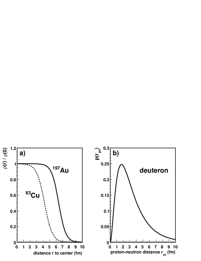
Figure 1: Density distributions for nuclei used at RHIC (a) and distribution of the proton-neutron distance in the deuteron as given by the Hulthen wave function (b).

In all calculations of geometric parameters using a Glauber approach, some experimental data must be given as model inputs. The two most important are the nuclear charge densities measured in low-energy electron scattering experiments and the energy dependence of the inelastic nucleon-nucleon cross section.

2.2.1 Nuclear Charge Densities

The nucleon density is usually parameterized by a Fermi distribution with three parameters:

$$\rho(r)=\rho_{0}\cdot\frac{1+w(r/R)^{2}}{1+\exp\left(\frac{r-R}{a}\right)}$$ (1)

where $\rho_{0}$ corresponds to the nucleon density in the center of the nucleus, $R$ corresponds to the nuclear radius, $a$ to the “skin depth” and $w$ characterizes deviations from a spherical shape. For ¹⁹⁷Au ($R=6.38$ fm; $a=0.535$ fm; $w=0$) and ⁶³Cu ($R=4.20641$ fm; $a=0.5977$ fm; $w=0$), the nuclei so far employed at RHIC, $\rho(r)/\rho_{0}$ is shown in Fig. 1a with the Fermi distribution parameters as given in ref. [22, 23]. In the Monte Carlo procedure the radius of a nucleon is randomly drawn from the distribution $4\pi r^{2}\,\rho(r)$ (where the absolute normalization is of course irrelevant).

At RHIC, effects of cold nuclear matter have been studied with the aid of d+Au collisions. In the Monte Carlo calculations the deuteron wave function was represented by the Hulthén form [24, 25]

$$\phi(r_{\mathrm{pn}})=\frac{1}{\sqrt{2\pi}}\frac{\sqrt{ab(a+b)}}{b-a}\cdot\frac{e^{-a\,r_{\mathrm{pn}}}-e^{-b\,r_{\mathrm{pn}}}}{r_{\mathrm{pn}}}$$ (2)

with parameters $a=0.228$ fm^-1 and $b=1.18$ fm^-1 [26]. The variable $r_{\mathrm{pn}}$ in Eq. 2 denotes the distance between the proton and the neutron. Accordingly, $r_{\mathrm{pn}}$ was drawn from the distribution $p(r_{\mathrm{pn}})=4\pi r_{\mathrm{pn}}^{2}\phi^{2}(r_{\mathrm{pn}})$ which is shown in Fig. 1b.

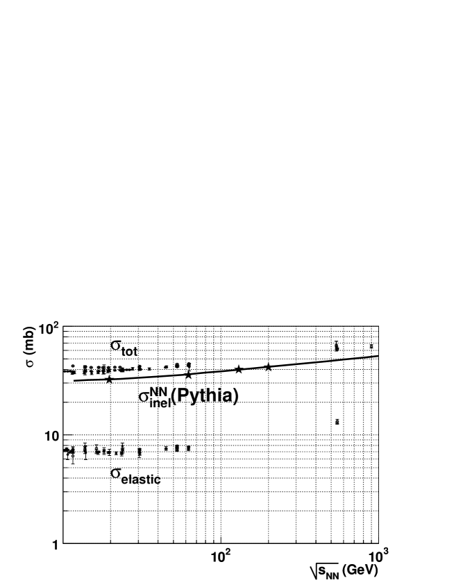
Figure 2: Inelastic nucleon-nucleon cross section $\sigma_{\mathrm{inel}}^{\mathrm{NN}}$ as parameterized by Pythia [34, 35] (solid line) along with data on total and elastic nucleon-nucleon cross sections as function of $\sqrt{s}$ [36]. The stars indicate nucleon-nucleon cross section used for Glauber Monte Carlo calculations at RHIC ($\sigma_{\mathrm{inel}}^{\mathrm{NN}}=$ 32.3, 35.6, 40, and 42 mb at $\sqrt{s_{\mathrm{NN}}}=$ 19.6, 62.4, 130, and 200 GeV)

2.2.2 Inelastic Nucleon-Nucleon Cross Section ($\sigma^{\mathrm{NN}}_{\mathrm{inel}}$)

In the context of high energy nuclear collisions, we are typically interested in multiparticle nucleon-nucleon processes. As the cross section involves processes with low momentum transfer, it is impossible to calculate this using perturbative QCD. Thus, the measured inelastic nucleon-nucleon cross section ($\sigma^{\mathrm{NN}}_{\mathrm{inel}}$) is used as an input, and provides the only non-trivial beam-energy dependence for Glauber calculations. From $\sqrt{s_{\mathrm{NN}}}\sim 20$ GeV (CERN SPS) to $\sqrt{s_{\mathrm{NN}}}=200$ GeV (RHIC) $\sigma^{\mathrm{NN}}_{\mathrm{inel}}$ increases from $\sim 32$ mb to $\sim 42$ mb as shown in Fig. 2. Diffractive and elastic processes, which are typically ignored in high energy multiparticle nuclear collisions, are generally active out to large impact parameters, and thus require full quantum mechanical wave functions.

2.3 Optical-limit Approximation

The Glauber Model views the collision of two nuclei in terms of the individual interactions of the constituent nucleons (see, e.g., Ref. [27]). In the optical limit, the overall phase shift of the incoming wave is taken as a sum over all possible two-nucleon (complex) phase shifts, with the imaginary part of the phase shifts related to the nucleon-nucleon scattering cross section through the optical theorem[28, 29]. The model assumes that at sufficiently high energies, these nucleons will carry sufficient momentum that they will be essentially undeflected as the nuclei pass through each other. It is also assumed that the nucleons move independently in the nucleus and that the size of the nucleus is large compared to the extent of the nucleon-nucleon force. The hypothesis of independent linear trajectories of the constituent nucleons makes it possible to develop simple analytic expressions for the nucleus-nucleus interaction cross section and for the number of interacting nucleons and the number of nucleon-nucleon collisions in terms of the basic nucleon-nucleon cross section.

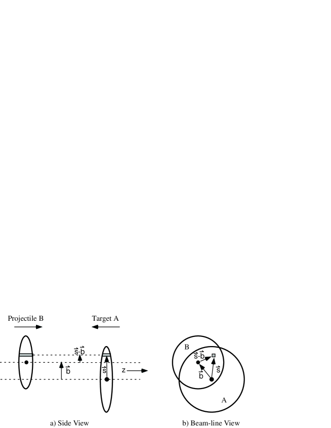
Figure 3: Schematic representation of the Optical Glauber Model geometry, with transverse (a) and longitudinal (b) views.

Consider Fig. 3. Two heavy-ions, “target” A and “projectile” B are shown colliding at relativistic speeds with impact parameter $\bf{b}$ (for colliding beam experiments the distinction between the target and projectile nuclei is a matter of convenience). We focus on the two flux tubes located at a displacement $\bf{s}$ with respect to the center of the target nucleus and a distance $\bf{s}-\bf{b}$ from the center of the projectile. During the collision these tubes overlap. The probability per unit transverse area of a given nucleon being located in the target flux tube is $\hat{T}_{A}\left(\bf{s}\right)=\int{\hat{\rho}_{A}({\bf s},z_{A})dz_{A}}$, where $\hat{\rho}_{A}\left({\bf s},z_{A}\right)$ is the probability per unit volume, normalized to unity, for finding the nucleon at location $\left({\bf s},z_{A}\right)$. A similar expression follows for the projectile nucleon. The product $\hat{T}_{A}\left({\bf s}\right)\hat{T}_{B}\left(\bf{s}-\bf{b}\right)d^{2}s$ then gives the joint probability per unit area of nucleons being located in the respective overlapping target and projectile flux tubes of differential area $d^{2}s$. Integrating this product over all values of $\bf{s}$ defines the “thickness function” $\hat{T}\left(\bf{b}\right)$, with

$$\hat{T}_{AB}\left(\bf{b}\right)=\int{\hat{T}_{A}\left(\bf{s}\right)\hat{T}_{B}\left(\bf{s}-\bf{b}\right)}d^{2}s.$$ (3)

Notice that $\hat{T}\left(\bf{b}\right)$ has the unit of inverse area. We can interpret this as the effective overlap area for which a specific nucleon in A can interact with a given nucleon in B. The probability of an interaction occurring is then $\hat{T}\left(\bf{b}\right)\sigma^{\mathrm{NN}}_{\mathrm{inel}}$, where $\sigma^{\mathrm{NN}}_{\mathrm{inel}}$ is the nucleon-nucleon inelastic cross section. Elastic processes lead to very little energy loss and are consequently not considered in the Glauber-model calculations. Once the probably of a given nucleon-nucleon interaction has been found, the probably of having n such interactions between nucleus A (with $A$ nucleons) and B (with $B$ nucleons) is given as a binomial distribution,

$$P\left(n,\bf{b}\right)=\left({\matrix{{AB}\cr n\cr}}\right)\left[\hat{T}_{AB}\left(\bf{b}\right)\sigma^{\mathrm{NN}}_{\mathrm{inel}}\right]^{n}\left[{1-\hat{T}_{AB}\left(\bf{b}\right)\sigma^{\mathrm{NN}}_{\mathrm{inel}}}\right]^{AB-n}$$ (4)

where the first term is the number of combinations for finding $n$ collisions out of $AB$ possible nucleon-nucleon interactions, the second term the probability for having exactly $n$ collisions, and the last term is the probability of exactly $AB-n$ misses.

Based on this probability distribution, a number of useful reactions quantities can be found. The total probability of an interaction between A and B is

$${{d^{2}\sigma^{\mathrm{A+B}}_{\mathrm{inel}}}\over{db^{2}}}\equiv p^{\mathrm{A+B}}_{\mathrm{inel}}(b)=\sum\limits_{n=1}^{AB}{P\left({n,\mathord{\buildrel{\lower 3.0pt\hbox{$\scriptscriptstyle\rightharpoonup$}}\over{b}}}\right)}=1-\left[{1-\hat{T}_{AB}\left(\bf{b}\right)\sigma^{\mathrm{NN}}_{\mathrm{inel}}}\right]^{AB}.$$ (5)

The vector impact parameter can be replaced by a scalar distance if the nuclei are not polarized. In this case, the total cross section can be found as

$$\sigma^{\mathrm{A+B}}_{\mathrm{inel}}=\int\limits_{0}^{\infty}{2\pi bdb\left\{{1-\left[{1-\hat{T}_{AB}\left(b\right)\sigma^{\mathrm{NN}}_{\mathrm{inel}}}\right]^{AB}}\right\}}$$ (6)

The total number of nucleon-nucleon collisions is

$$N_{\mathrm{coll}}\left(b\right)=\sum\limits_{n=1}^{AB}{nP\left({n,b}\right)=AB\hat{T}_{AB}\left(b\right)\sigma^{\mathrm{NN}}_{\mathrm{inel}}}$$ (7)

using the result for the mean of a binomial distribution. The number of nucleons in the target and projectile nuclei that interact is called either the “number of participants” or the “number of wounded nucleons”. The number of participants (or wounded nucleons) at impact parameter b is given by [15, 30]

$$N_{\mathrm{part}}\left(\bf{b}\right) = A\int{\hat{T}_{A}\left(\bf{s}\right)\left\{{1-\left[{1-\hat{T}_{B}\left({\bf{s}-{\bf b}}\right)\sigma^{\mathrm{NN}}_{\mathrm{inel}}}\right]^{B}}\right\}d^{2}s+}$$ (8)

$$B\int{\hat{T}_{B}\left({\bf{s}-\bf{b}}\right)\left\{{1-\left[{1-\hat{T}_{A}\left({\bf{s}}\right)\sigma^{\mathrm{NN}}_{\mathrm{inel}}}\right]^{A}}\right\}d^{2}s},$$

where it can be noted that the integral over the bracketed terms give the respective inelastic cross sections for nucleon-nucleus collisions:

$$\sigma^{\mathrm{A\left(B\right)}}_{\mathrm{inel}}=\int{d^{2}s\left\{{1-\left[{1-\sigma^{\mathrm{NN}}_{\mathrm{inel}}\hat{T}_{A(B)}\left({\bf{s}}\right)}\right]^{A(B)}}\right\}}.$$ (9)

The optical form of the Glauber theory is based on continuous nucleon density distributions. The theory does not locate nucleons at specific spatial coordinates, as is the case for the Monte Carlo formulation that is discussed in the next section. This difference between the optical and Monte Carlo approaches can lead to subtle differences in calculated results, as will be discussed below.

2.4 Glauber Monte Carlo approach

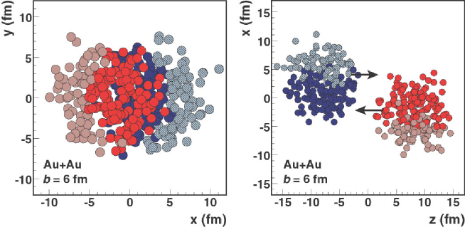
Figure 4: Glauber Monte Carlo event (Au+Au at $\sqrt{s_{\mathrm{NN}}}=200$ GeV with impact parameter $b=6$ fm) viewed in the transverse plane (left panel) and along the beam axis (right panel). The nucleons are drawn with a radius $\sqrt{\sigma^{\mathrm{NN}}_{\mathrm{inel}}/\pi}/2$. Darker disks represent participating nucleons.

The virtue of the Monte Carlo approach for the calculation of geometry related quantities like $\langle N_{\mathrm{part}}\rangle$ and $\langle N_{\mathrm{coll}}\rangle$ is its simplicity. Moreover, it is possible to simulate experimentally observable quantities like the charged particle multiplicity and to apply similar centrality cuts as in the analysis of real data. In the Monte Carlo ansatz the two colliding nuclei are assembled in the computer by distributing the $A$ nucleons of nucleus A and $B$ nucleons of nucleons B in three-dimensional coordinate system according to the respective nuclear density distribution. A random impact parameter $b$ is then drawn from the distribution $\mathrm{d}\sigma/\mathrm{d}b=2\pi b$. A nucleus-nucleus collision is treated as a sequence of independent binary nucleon-nucleon collisions, i.e., the nucleons travel on straight-line trajectories and the inelastic nucleon-nucleon cross-section is assumed to be independent of the number of collisions a nucleon underwent before. In the simplest version of the Monte Carlo approach a nucleon-nucleon collision takes place if their distance $d$ in the plane orthogonal to the beam axis satisfies

$$d\leq\sqrt{\sigma^{\mathrm{NN}}_{\mathrm{inel}}/\pi}$$ (10)

where $\sigma^{\mathrm{NN}}_{\mathrm{inel}}$ is the total inelastic nucleon-nucleon cross-section. As an alternative to the black-disk nucleon-nucleon overlap function, e.g., a Gaussian overlap function can be used [31].

An illustration of a Glauber Monte Carlo event for a Au+Au collision with impact parameter $b=6$ fm is shown in Fig. 4. The average number of participating nucleons and binary nucleon-nucleon collisions and other quantities are then determined by simulating many nucleus-nucleus collisions.

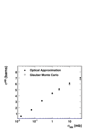
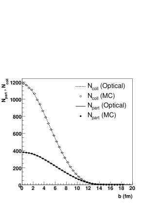
Figure 5: (left) Total cross section, calculated in the optical approximation and with a Glauber Monte Carlo, both with identical nuclear parameters, as a function of $\sigma^{\mathrm{NN}}_{\mathrm{inel}}$, the nucleon-nucleon inelastic cross section. (right) $N_{\mathrm{coll}}$ and $N_{\mathrm{part}}$ as a function of impact parameter, calculated in the optical approximation (lines) and with a Glauber Monte Carlo (symbols). The two are essentially identical out to $b=2R_{A}$.

2.5 Differences between Optical and Monte Carlo Approaches

It is not always remembered that the various integrals used to calculated physical observables in the “Glauber Model” are predicated on a particular approximation called the optical limit. This limit assumes that scattering amplitudes can be described by an eikonal approach, where the incoming nucleons see the target as a smooth density. This approach captures many features of the collision process, but does not completely capture the physics of the total cross section. Thus, it tends to lead to distortions in the estimation of $N_{\mathrm{part}}$ and $N_{\mathrm{coll}}$ compared to similar estimations using the Glauber Monte Carlo approach.

This can be seen by simply looking at the relevant integrals. The full (2A+2B+2)-dimensional integral to calculate the total cross section is [15]:

$$\sigma_{AB}=\int d^{2}b\int d^{2}s^{A}_{1}\cdots d^{2}s^{A}_{A}d^{2}s^{B}_{1}\cdots d^{2}s^{B}_{B}\times$$

$$\hat{T}_{A}({\bf s^{A}_{1}})\cdots\hat{T}_{A}({\bf s^{A}_{A}})\hat{T}_{B}({\bf s^{B}_{1}})\cdots\hat{T}_{B}({\bf s^{B}_{B}})\times$$ (11)

$$\left\{1-\prod_{j=1}^{B}\prod_{i=1}^{A}[1-\hat{\sigma}({\bf b-s^{A}_{i}+s^{B}_{j}})]\right\}$$

where $\hat{\sigma}({\bf s})$ is normalized such that $\int d^{2}s\hat{\sigma}({\bf s})=\sigma^{\mathrm{NN}}_{\mathrm{inel}}$, while the optical limit version of the same calculation is (cf. Equation 6):

$$\sigma_{AB}=\int d^{2}b\left\{1-[1-\sigma^{\mathrm{NN}}_{\mathrm{inel}}\hat{T}_{AB}(b)]^{AB}\right\}$$ (12)

These expressions are generally expected to be the same for large A (and B) and/or when $\sigma^{\mathrm{NN}}_{\mathrm{inel}}$ is sufficiently small [15]. The main difference between the two is that many terms in the full calculation are missing in the optical limit calculation. These are the terms which describe local density fluctuations event-by-event. Thus, in the optical limit, each nucleon in the projectile sees the oncoming target as a smooth density.

One can test this interpretation to first order by plotting the total cross section as a function of $\sigma^{\mathrm{NN}}_{\mathrm{inel}}$ for an optical limit calculation as well as a GMC calculation with the same parameters, as shown in the left panel of Fig. 5. One sees that as the nucleon-nucleon cross section becomes more point-like, the optical and GMC cross sections converge. This confirms the general suspicion that it is the ability of GMC calculations to introduce “shadowing” corrections that reduces the cross section relative to the optical calculations [11]

And yet, when calculating simple geometric quantities like $N_{\mathrm{part}}$ and $N_{\mathrm{coll}}$ as a function of impact parameter, there is little difference between the two calculations, as shown in the right panel of Fig. 5. The only substantial difference comes at the highest impact parameters, something which will be discussed in Section 3.4.1. Fluctuations are also sensitive to this difference, but there is insufficient room in this review to discuss more recent developments [32].

2.6 Glauber Model Systematics

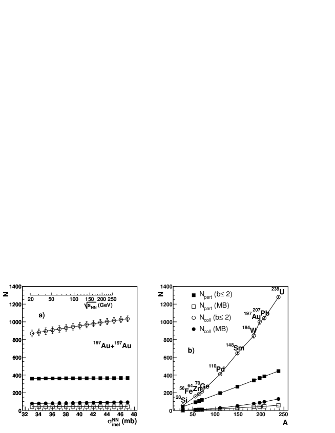
Figure 6: a) Dependence of $N_{\mathrm{part}}$ and $N_{\mathrm{coll}}$ on $\sigma^{\mathrm{NN}}_{\mathrm{inel}}$ for central ($b\leq 2~{}\mathrm{fm}$) and minimum bias (MB) events for the $\mathrm{{}^{197}Au+^{197}Au}$ reaction. b) Dependence of these values on the system size, with $\sigma^{\mathrm{NN}}_{\mathrm{inel}}=42~{}\mathrm{mb}$.

As discussed above, the Glauber model depends on the nucleon-nucleon inelastic cross $\sigma^{\mathrm{NN}}_{\mathrm{inel}}$ section and the geometry of the interacting nuclei. In turn, $\sigma^{\mathrm{NN}}_{\mathrm{inel}}$ depends on the energy of the reaction, as shown in Fig. 2, and the geometry depends on the number of nucleons in the target and projectile.

Figure 6a shows the effect of changing $\sigma^{\mathrm{NN}}_{\mathrm{inel}}$ on the calculated values of the number of participant ($N_{\mathrm{part}}$) and the number of collisions ($N_{\mathrm{coll}}$) for $\mathrm{{}^{197}Au+^{197}Au}$ reaction over the range of $\sigma^{\mathrm{NN}}_{\mathrm{inel}}$ values relevant at RHIC. The secondary axis shows the values of $\sqrt{s_{\mathrm{NN}}}$ corresponding to the $\sigma^{\mathrm{NN}}_{\mathrm{inel}}$ values. The values are shown for central events, with impact parameter $b<2~{}\mathrm{fm}$, and for a minimum bias throw of events. The error bars, which only extend beyond the symbol size for the $N_{\mathrm{coll}}$($b<2~{}\mathrm{fm}$) results, are based on an assumed uncertainty of $\sigma_{\mathrm{inel}}^{\mathrm{NN}}$ at a given energy of 3 mb. In general, one finds that the Glauber calculations show only a weak energy dependence over the energy range covered by the RHIC accelerator.

Fig. 6b shows dependence of $N_{\mathrm{part}}$ and $N_{\mathrm{coll}}$ on the system size for central and MB events, with values calculated for identical particle collisions of the indicated systems at a fixed value of $\sigma^{\mathrm{NN}}_{\mathrm{inel}}=42~{}\mathrm{mb}$ (corresponding to $\sqrt{s_{\mathrm{NN}}}=200~{}\mathrm{GeV}$). Since the Glauber Model is largely dependent on the geometry of the colliding nuclei, some simple scalings can be expected for $N_{\mathrm{part}}$ and $N_{\mathrm{coll}}$.

$N_{\mathrm{part}}$ should scale with the volume of the interaction region. In Fig. 6 this is seen by the linear dependence of $N_{\mathrm{part}}$ for central collisions on $A$, where the common volume $V$ of the largely overlapping nuclei in central collisions is proportional to $A$ for a saturated nuclear density. In a collisions of two equal nuclei (A+A) the average number of collisions per participant scales as the length $l_{z}\propto N_{\mathrm{part}}^{1/3}$ of the interaction volume along the beam direction so that the number of collisions roughly follows

$$N_{\mathrm{coll}}\propto N_{\mathrm{part}}^{4/3}\$$ (13)

independent of the size of the nuclei. This scaling relationship is demonstrated in Fig. 7 where $N_{\mathrm{coll}}/N_{\mathrm{part}}^{\mathrm{4/3}}$ is plotted as a function of $N_{\mathrm{part}}$ for the systems shown in Fig. 6b. The result is confirmed experimentally in ref. [33] where the $\mathrm{Cu+Cu}$ and $\mathrm{Au+Au}$ systems are compared. The geometric nature of the Glauber Model is evident.

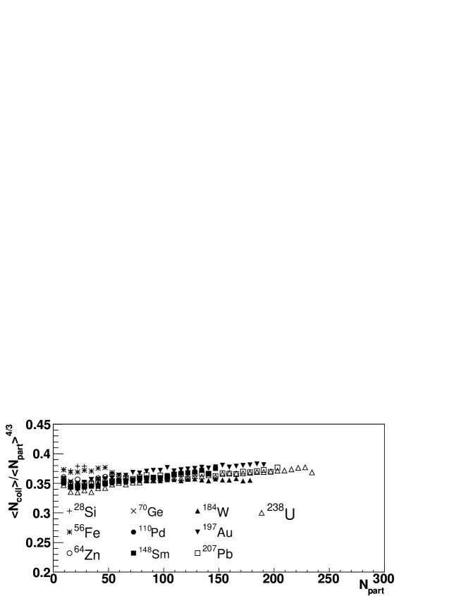
Figure 7: Geometric scaling behavior of $N_{\mathrm{coll}}$ as discussed in the text. The calculations are done with $\sigma^{\mathrm{NN}}_{\mathrm{inel}}=42~{}\mathrm{mb}$.

3 Relating the Glauber Model to Experimental Data

Unfortunately, neither $N_{\mathrm{part}}$ nor $N_{\mathrm{coll}}$ can be directly measured in a RHIC experiment. Mean values of such quantities can be extracted for classes of ($N_{\mathrm{evt}}$) measured events via a mapping procedure. Typically a measured distribution (e.g., $\mathrm{d}N_{\mathrm{evt}}/\mathrm{d}N_{\mathrm{ch}}$) is mapped to the corresponding distribution obtained from phenomenological Glauber calculations. This is done by defining “centrality classes” in both the measured and calculated distributions and then connecting the mean values from the same centrality class in the two distributions. The specifics of this mapping procedure differ both between experiments as well as between collision systems within a given experiment. Herein we briefly summarize the principles and various implementations of centrality definition.

3.1 Methodology

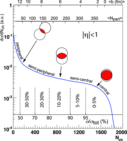
Figure 8: A cartoon example of the correlation of the final state observable $N_{\mathrm{ch}}$ with Glauber calculated quantities ($b$, $N_{\mathrm{part}}$). The plotted distribution and various values are illustrative and not actual measurements (T. Ullrich, private communication).

The basic assumption underlying centrality classes is that the impact parameter $b$ is monotonically related to particle multiplicity, both at mid and forward rapidity. For large $b$ events (“peripheral”) we expect low multiplicity at mid-rapidity, and a large number of spectator nucleons at beam rapidity, whereas for small $b$ events (“central”) we expect large multiplicity at mid-rapidity and a small number of spectator nucleons at beam rapidity (Figure 8). In the simplest case, one measures the per-event charged particle multiplicity ($\mathrm{d}N_{\mathrm{evt}}/\mathrm{d}N_{\mathrm{ch}}$) for an ensemble of events. Once the total integral of the distribution is known, centrality classes are defined by binning the distribution based upon the fraction of the total integral. The dashed vertical lines in Figure 8 represent a typical binning. The same procedure is then applied to a calculated distribution, often derived from a large number of Monte Carlo trials. For each centrality class, the mean value of Glauber quantities (e.g., $\langle N_{part}\rangle$) for the Monte Carlo events within the bin (e.g., 5-10%) is calculated. Potential complications to this straightforward procedure arise from various sources: event selection, uncertainty in the total measured cross section, fluctuations in both the measured and calculated distributions, and finite kinematic acceptance.

3.1.1 Event Selection

All four RHIC experiments share a common detector to select minimum bias (MB) heavy ion events. The Zero Degree Calorimeters (ZDCs) are small acceptance hadronic calorimeters with angular coverage of $\theta\leq 2$ mrad with respect to the beam axis [9]. Situated behind the charged particle steering DX magnets of RHIC, the ZDCs are primarily sensitive to neutral spectators. For Au+Au collisions at $\sqrt{s_{\mathrm{NN}}}=130$ GeV and above, the ZDCs are $\sim 100$% efficient for inelastic collisions, thus providing an excellent MB trigger. The RHIC experiments often apply an online timing cut to select events within a given primary vertex interval ($\sim|z_{\mathrm{vertex}}|<$30 cm). Further coincidence with fast detectors near mid-rapidity are often also used to suppress background events such as beam-gas collisions. Experiment specific event selection is described in detail in section 3.2.

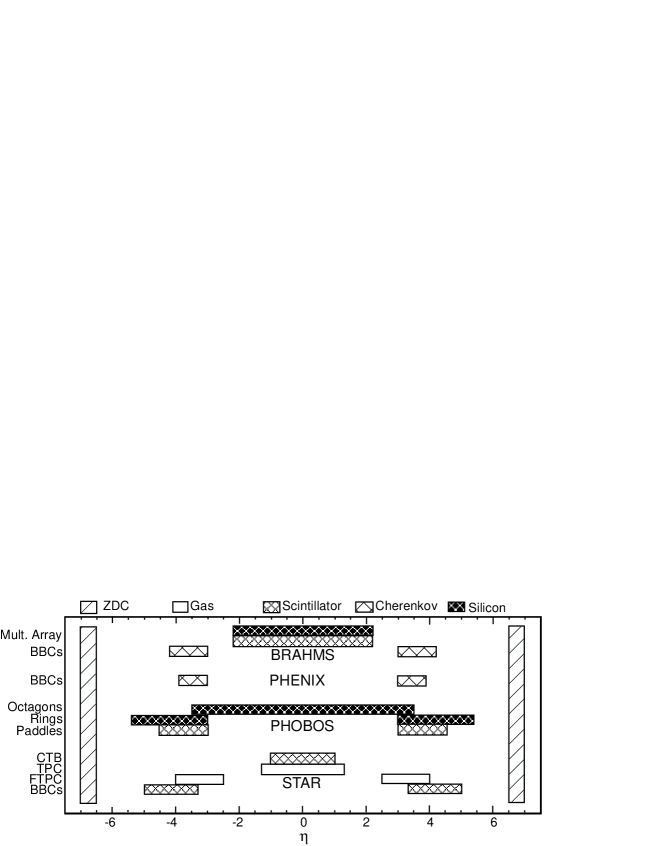
Figure 9: Pseudorapidity coverage of the centrality selection detectors of the 4 RHIC experiments. Top to bottom: BRAHMS, PHENIX, PHOBOS, STAR.

Figure 9 displays the pseudorapidity coverage of the suite of subsystems used to define centrality (both offline and at the trigger level) [37, 38, 39, 40]. With the exception of the STAR TPC and FTPCs, all other subsystems are intrinsically fast and available for event triggering.

3.1.2 Centrality Observables

In minimum bias p+p and p+$\bar{\mathrm{p}}$ collisions at high energy, the charged particle multiplicity $\mathrm{d}N_{\mathrm{evt}}/\mathrm{d}N_{\mathrm{ch}}$ has been measured over a wide range of rapidity and is well described by a negative binomial distribution [41]. However, the multiplicity is also known to scale with the hardness ($q^{2}$) of the collision – the multiplicity for hard jet events is significantly higher than that of MB collisions. In heavy ion collisions, we manipulate the fact that the majority of the initial state nucleon-nucleon collisions will be analogous to minimum bias p+p collisions, with a small perturbation from much rarer hard interactions. The final integrated multiplicity of heavy ion events is then roughly described as a superposition of many negative binomial distributions, which quickly approaches the Gaussian limit.

$N_{\mathrm{ch}}$ can be measured offline by counting charged tracks (e.g, STAR TPC) or estimated online from the total energy deposited in a detector divided by the typical energy deposition per charged particle (e.g., PHOBOS Paddles).

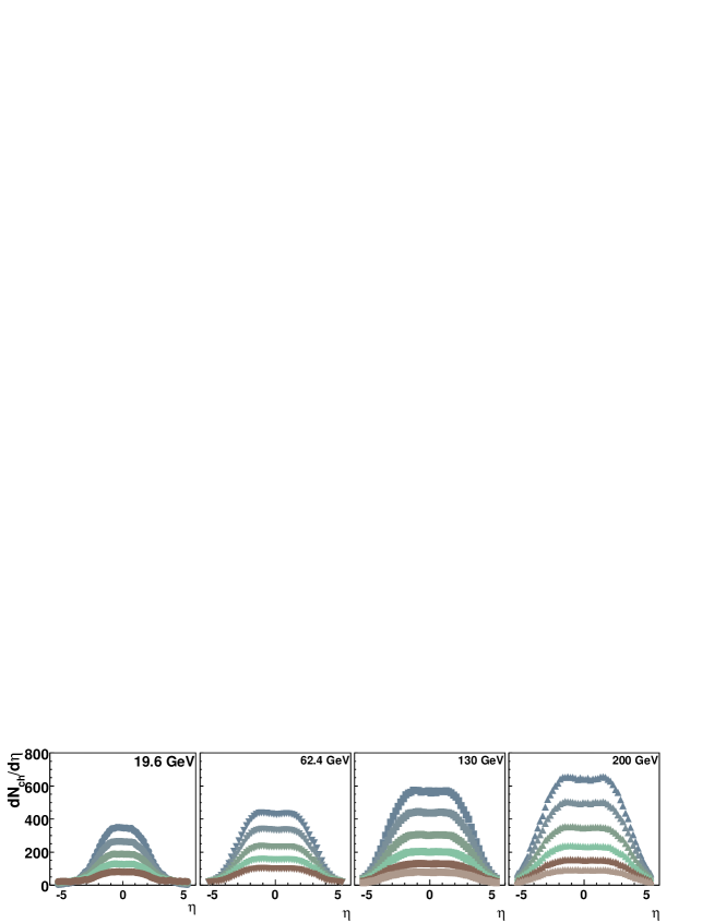
Figure 10: Charged particle multiplicity (PHOBOS) in Au+Au collisions at various center-of-mass energies for $|\eta|<5$ [57, 58]. The different colors represent different centrality selections.

As shown in Figure 9, there is a wide variation in the acceptance of various centrality detectors at RHIC. PHOBOS, with the largest acceptance in $\eta$, is well suited to measure $\frac{\mathrm{d}^{2}N_{\mathrm{evt}}}{\mathrm{d}N_{\mathrm{ch}}\mathrm{d}\eta}$ (Figure 10). These data illustrate two key features of particle production in nucleus-nucleus collisions. At a fixed beam energy, there is no dramatic change in shape as the centrality changes. However reducing the beam energy does change the shape substantially, since the maximum rapidity varies as $\ln(\sqrt{s_{\mathrm{NN}}})$. Thus, the same trigger detector may have a very different overall efficiency at different beam energies.

$N_{\mathrm{ch}}$ can be simulated via various methods, but all require the coupling of a Glauber calculation to a model of charged particle production, either dynamic (e.g. HIJING [19]) or static (randomly sampled from a Gaussian, Poisson, or negative binomial). Most follow the general prescription that the multiplicity scales approximately with $N_{\mathrm{part}}$. For an optical Glauber calculation, simulated multiplicity ($N_{\mathrm{ch}}^{\mathrm{sim}}$) can be calculated semi-analytically assuming that each participant contributes a given value of $N_{\mathrm{ch}}$ which is typically drawn from one of the aforementioned static probability distributions [42]. The same can be done for a Monte Carlo Glauber simulation with the added advantage that the detector response to such “events” can be simulated, thus enabling an apples-to-apples comparison of simulated and measured $N_{\mathrm{ch}}$ distributions. Various dynamical models of heavy ion collisions exist and can also be coupled to detector simulations. In all cases, the exact value of $N_{\mathrm{part}}$, $N_{\mathrm{coll}}$, $b$, and $N_{\mathrm{ch}}^{\mathrm{sim}}$ are known for each event.

3.1.3 Dividing by Percentile of Total Inelastic Cross Section

With a measured and simulated $\mathrm{d}N_{\mathrm{evt}}/\mathrm{d}N_{\mathrm{ch}}$ distribution in hand, one can then perform the mapping procedure to extract mean values. Suppose that the measured and simulated distributions are both one dimensional histograms. For each histogram, the total integral is calculated and centrality classes are defined in terms of fraction of the total integral. Typically the integration is performed from large values of $N_{\mathrm{ch}}$ to small. For example, the 10-20% most central class is defined by boundaries $n_{10}$ and $n_{20}$ which satisfy

$$\frac{\int_{\infty}^{n_{10}}\frac{\mathrm{d}N_{\mathrm{evt}}}{\mathrm{d}N_{\mathrm{ch}}}\,\mathrm{d}N_{\mathrm{ch}}}{\int_{\infty}^{0}\frac{\mathrm{d}N_{\mathrm{evt}}}{\mathrm{d}N_{\mathrm{ch}}}\,\mathrm{d}N_{\mathrm{ch}}}=0.1\textrm{ and }\frac{\int_{\infty}^{n_{20}}\frac{\mathrm{d}N_{\mathrm{evt}}}{\mathrm{d}N_{\mathrm{ch}}}\,\mathrm{d}N_{\mathrm{ch}}}{\int_{\infty}^{0}\frac{\mathrm{d}N_{\mathrm{evt}}}{\mathrm{d}N_{\mathrm{ch}}}\,\mathrm{d}N_{\mathrm{ch}}}=0.2\,.$$ (14)

See, for example, Figure 8. The same procedure is performed on both the measured and simulated distribution. We note explicitly that $n_{i}^{\mathrm{measured}}$ need not equal $n_{i}^{\mathrm{simulated}}$. This non-trivial fact implies that the mapping procedure is robust to an overall scaling of the simulated $N_{\mathrm{ch}}$ distribution compared to the measured distribution.

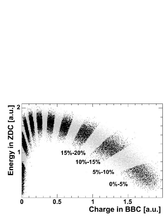
Figure 11: Spectator energy deposition in the ZDCs as a function of charged particle multiplicity in the BBCs (PHENIX).

One can extend the centrality classification beyond one dimension by studying the correlation of beam rapidity spectator multiplicity with mid-rapidity particle production (Figure 11). Although the distribution is somewhat asymmetric, the naive expectations of Section 3.1 are clearly upheld and the mapping procedure proceeds as in the 1-d case.

Once a centrality class is defined in simulation, the mean values of quantities such as $N_{\mathrm{part}}$ can be calculated for events that fall in that centrality bin. Systematic uncertainty in the total measured cross section propagates into a leading systematic uncertainty on the Glauber quantities extracted via the mapping process. This uncertainty can be directly propagated by varying the value of the denominator in Equation 14 accordingly and recalculating $\langle N_{\mathrm{part}}\rangle$, etc. For example, for Au+Au collisions at $\sqrt{s_{\mathrm{NN}}}=200$ GeV in the 10-20% (60-80%) most central bin, the STAR collaboration quotes values of $\langle N_{\mathrm{part}}\rangle\approx$ 234 (21) with an uncertainty of $\sim$ 6 (5) from the 5% uncertainty on the total cross section alone [43]. Clearly the uncertainty in total cross section becomes increasingly important as one approaches the most peripheral collisions.

3.2 Experimental Details

3.2.1 BRAHMS

The BRAHMS experiment uses the charged particle multiplicity observed in a pseudorapidity range of $-2.2\leq\eta\leq 2.2$ to determine reaction centrality [44, 45, 46]. The multiplicities are measured in a “multiplicity array” consisting of an inner barrel of Si strip detectors (SiMA) and an outer barrel of plastic scintillator “tile” detectors (TMA) [37, 47] for collisions within 36 cm of the nominal vertex location. Both arrays cover the same pseudorapidity range for collisions at the nominal vertex. “Beam-Beam”-counter arrays (BBC)located on either side of the nominal interaction point at a distance of 2.2 m of the nominal vertex extend the pseudorapidity coverage for measuring charge-particle pseudorapidity densities. These arrays consist of Cherenkov UV-transmitting plastic radiators coupled to photomultiplier tubes.

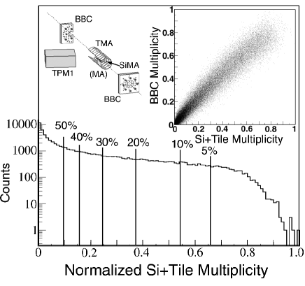
Figure 12: Normalized multiplicity distribution for the ${}^{197}\rm{Au}+^{197}\rm{Au}$ reaction at $\sqrt{s_{\mathrm{NN}}}=130~{}\rm{GeV}$ measured in the BRAHMS multiplicity array[44]. The insert shows the correlation pattern of multiplicities measured in the Beam-Beam Counter arrays and the multiplicity array. The vertical lines indicate multiplicity values associated with the indicated centrality cuts.

Figure 12 shows the normalized multiplicity distribution measured in the multiplicity array for the ${}^{197}\rm{Au}+^{197}\rm{Au}$ reaction at $\sqrt{s_{\mathrm{NN}}}=130~{}\rm{GeV}$. The insert shows a correlation plot of the multiplicity measured in the Beam-Beam counter array and that in the multiplicity array. The vertical lines indicate the multiplicities corresponding to the indicated centrality values.

The BRAHMS reference multiplicity distribution requires coincident signals in the experiment’s two ZDC detectors, an interaction vertex located within 30 cm of the nominal vertex location, and that there be at least four “hits” in the TMA. This additional requirement largely removes background contributions from beam-residual gas interactions and from very peripheral collisions involving only electromagnetic processes. The collision vertex can be determined by either the BBC-arrays, the ZDC counters, or a time-projection chamber that is part of a mid-rapidity spectrometer arm (TPM1 in Fig. 12).

A simulation of the experimental response based on realistic GEANT3 simulations [48] and using the HIJING Monte Carlo event generator [19] for input was used to estimate the fraction of the inelastic scattering yield that was missed in the experiment’s minimum-bias event selection. Multiplicity spectra using the simulated events are compared to the experimental spectra. The shapes of the spectra are found to agree very well for an extended range of multiplicities in the TMA array above the threshold multiplicity set for the event selection. The simulated events are then used to extrapolate the experimental spectrum below the threshold. Using this procedure, it is estimated that the minimum-bias event selection criteria selects $(93\pm 3){\rm{\%}}$ of the total nuclear cross section for Au+Au collisions at $\sqrt{s_{\mathrm{NN}}}=200{\kern 1.0pt}\;{\rm{GeV}}$, down to $(87\pm 7){\rm{\%}}$ for Cu+Cu collisions at $\sqrt{s_{\mathrm{NN}}}=62.4{\kern 1.0pt}\;{\rm{GeV}}$.

3.2.2 PHENIX

We consider two examples: Au+Au at $\sqrt{s_{\mathrm{NN}}}=200$ GeV and Cu+Cu at $\sqrt{s_{\mathrm{NN}}}=22.4$ GeV. The minimum bias trigger condition for Au+Au collisions at $\sqrt{s_{\mathrm{NN}}}=200$ GeV was based on Beam-Beam-Counters (BBCs) [38]. The two BBCs ($3.1\leq|\eta|\leq 3.9$) each consist of 64 photomultipliers which detect Cherenkov light produced by charged particles traversing quartz radiators. On the hardware level a minimum bias event was required to have at least 2 photomultiplier hits in each BBC. Some analyses only used events with an additional hardware coincidence of the two ZDCs. Moreover, the interaction vertex along the beam axis ($z$ axis) reconstructed based on the arrival time difference in the two BBCs was required to lie within $\pm 30$ cm of the nominal vertex.

The efficiency of accepting inelastic Au+Au collisions under the condition of having at least two photomultiplier hits in each BBC ($N_{\mathrm{PMT}}^{\mathrm{BBC}}\geq 2$) was determined with the aid of HIJING Monte Carlo events [19] and a detailed simulation of the BBC response [48]. With an offline vertex cut of $\pm 30$ cm these simulations yield an efficiency of $(92.3\pm 2)\,\%$ for Au+Au at $\sqrt{s_{\mathrm{NN}}}=200$ GeV [49]. The systematic uncertainties reflect uncertainties of (a) $\mathrm{d}N_{\mathrm{ch}}/\mathrm{d}y$ in HIJING, (b) the shape of the $z$-vertex distribution, and (c) the stability of the photomultiplier gains.

The additional requirement of a ZDC coincidence removes remaining background from beam-gas interactions, but possibly also leads to a small inefficiency for peripheral collisions. The efficiency of accepting real Au+Au collisions with $N_{\mathrm{PMT}}^{\mathrm{BBC}}\geq 2$ under the condition of a coincidence of the ZDCs was estimated to be $99^{+1.0}_{-1.5}$ %. Combining the efficiencies of the BBC and ZDC requirement as well as the offline vertex cut PHENIX finds that its sample of minimum bias events in Au+Au at $\sqrt{s_{\mathrm{NN}}}=200$ GeV corresponds to $91.4^{+2.5}_{-3.0}\,\%$ of the total inelastic cross section. Centrality classes were then defined by cuts on the two-dimensional distribution of the ZDC energy as a function of the BBC signal as shown in Figure 11.

As a second example we consider the centrality selection in Cu+Cu collisions at $\sqrt{s_{\mathrm{NN}}}=22.4$ GeV. At this energy the beam rapidity $y_{\mathrm{beam}}\approx 3.2$ lies within the pseudorapidity range of the BBCs. The BBCs were still used as minimum bias trigger detectors ($N_{\mathrm{PMT}}^{\mathrm{BBC}}\geq 1$ in both BBCs). However, a monotonic relation between the BBC signal and the impact parameter was no longer obvious. Thus, the hit multiplicity ($N_{\mathrm{PC1}}$) measured with a Pad Chamber detector [50] at mid-rapidity ($|\eta|\leq 0.35$) was used as centrality variable.

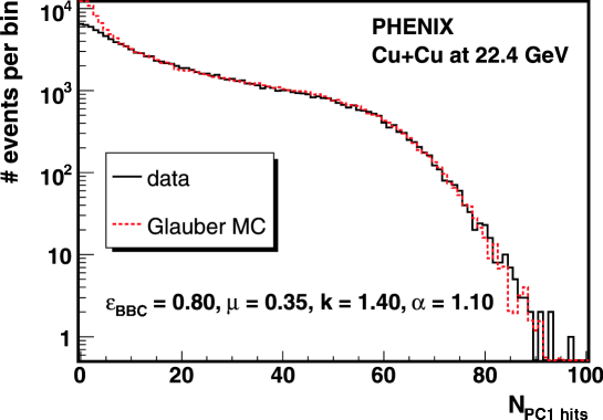
Figure 13: Measured and simulated distribution of the Pad Chamber 1 hit multiplicity used as centrality variable in Cu+Cu collisions at $\sqrt{s_{\mathrm{NN}}}=22.4$ GeV (PHENIX).

The PC1 multiplicity distribution was simulated based on a convolution of the $N_{\mathrm{part}}$ distribution from Glauber MC and a negative binomial distribution (NBD). A non-linear scaling of the average particle multiplicity with $N_{\mathrm{part}}$ was allowed: it was assumed that the number of independently decaying precursor particles (’ancestors’, $N_{\mathrm{ancestor}}$) is given by $N_{\mathrm{ancestor}}=N_{\mathrm{part}}^{\alpha}$. The number of measured PC1 hits per precursor particle was assumed follow a NBD:

$$P_{\mu,k}(n)=\frac{\Gamma(n+k)}{\Gamma(n+1)\,\Gamma(k)}\cdot\frac{(\mu/k)^{n}}{(\mu/k+1)^{n+k}}\,.$$ (15)

In a Glauber MC event the NBD was sampled $N_{\mathrm{ancestor}}$ times to obtain the simulated PC1 multiplicity for this event. The PC1 multiplicity distribution was simulated for a grid of values for $\mu$, $k$ , and $\alpha$ in order to find optimal values. Figure 13 shows the measured and simulated PC1 distribution along with the best estimate of the BBC trigger efficiency ($\varepsilon_{\mathrm{BBC}}\approx 0.8$) corresponding to the difference at small $N_{\mathrm{PC1}}$ (see [49] for a similar study in Au+Au collisions at $\sqrt{s_{\mathrm{NN}}}=19.6$ GeV). Given the good agreement between the measured and simulated distribution in Figure 13 centrality classes for Cu+Cu collisions at $\sqrt{s_{\mathrm{NN}}}=22.4$ GeV were defined by identical cuts on the measured and simulated $N_{\mathrm{PC1}}$.

3.2.3 PHOBOS

As discussed above, PHOBOS measures centrality with 2 sets of 16 scintillator paddle counters covering $3<|\eta|<4.5$ [39]. Good events are defined by having less than 4 ns time difference between the first hit impinging on each paddle counter (limiting the vertex range) and either a coincidence between the PHOBOS ZDCs or a high summed energy signal in the paddles (to avoid the slight inefficiency in the ZDCs at small impact parameter at low energies).

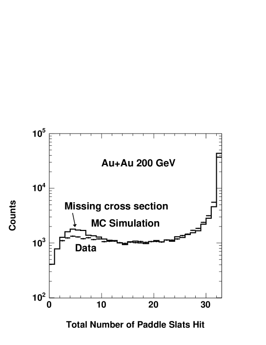
Figure 14: PHOBOS data showing the number of paddle slats hit by charged particles, out of 32 total, in triggered events. The data is compared with a full Monte Carlo simulation of unbiased HIJING events. The data is normalized around $N(slats)\sim 16$ in order to compare data and MC, to estimate the fraction of events lost to the trigger conditions.

PHOBOS estimates the observed fraction of the total cross section by measuring the distribution of the total number of paddle slats, as shown in Figure 14. Most of the variation in this quantity essentially measures the very low-multiplicity part of the multiplicity distribution, since the bulk of the events have sufficient multiplicity to fire all of the paddles simultaneously. The inefficiency is determined by matching the “plateau” structure in the data to that in HIJING, and measuring how many of the low multiplicity events are missed in the data relative to the MC calculation. This accounts for a variety of instrumental effects in an aggregate way, and the difference between the estimated value and 100% sets the scale for the systematic uncertainty.

The total detection efficiency for 200 GeV Au+Au collisions is found to be 97%, and 88% when requiring more than 2 slats hit on each set of 16 paddle counters. This last requirement dramatically reduces background events taken to tape, and the relative efficiency is straightforward to measure with the events triggered on a coincidence of 1 or more hits in each set of counters.

For events with much lower multiplicities and/or lower energies, both the multiplicity and rapidity reach are substantially smaller. This strongly impacts the efficiency of the paddle counters, and thus potentially distorts the centrality estimation. For these, PHOBOS uses the full distribution of multiplicities measured in several $\eta$ regions of the Octagon and Ring multiplicity counters, and matches them to the distributions measured in a MC simulation, typically HIJING. Once the overall multiplicity scale is fit, the difference in the integrals between data and MC gives a reasonable estimate of the fraction of observed total cross section.

3.2.4 STAR

STAR defines centrality classes for Cu+Cu and Au+Au (d+Au) using charged particle tracks reconstructed in the TPC (FTPC) over full azimuth and $|\eta|<0.5$ ($2.5<\eta<4$). Background events are removed by requiring the reconstruction of a primary vertex in addition to either a coincident ZDC (130/200 GeV Au+Au/Cu+Cu) or BBC (62.4 GeV Au+Au/Cu+Cu) signal. Vertex reconstruction inefficiency in low multiplicity events reduces the fraction of the total measured cross section to, e.g., $(95\pm 5)$% for 130 GeV Au+Au. For MB events, centrality is defined offline by binning the measured $\mathrm{d}N_{\mathrm{evt}}/\mathrm{d}N_{\mathrm{ch}}$ distribution by fraction of total cross section. Glauber calculations are performed using a Monte Carlo calculation. STAR enhances central events via an online trigger using a coincidence between the MB ZDC condition and large energy deposition in the Central Trigger Barrel (CTB), a set of 240 scintillating slats covering full azimuth and $-1<\eta<1$. After offline cuts the central trigger corresponds to the 0-5% most central class of events. STAR has several methods of extracting mean values of Glauber quantities.

(1) STAR reports little dependence on the mean values of $N_{\mathrm{part}}$ and $N_{\mathrm{coll}}$ extracted via the aforementioned mapping procedure when vastly different models of particle production were used to simulate the charged particle multiplicity. Thus, for many analyses (62.4/130/200 GeV Au+Au) STAR bypasses simulation of the multiplicity distribution and instead defines centrality bins from the Monte Carlo calculated $\mathrm{d}\sigma/\mathrm{d}N_{\mathrm{part}}$ and $\mathrm{d}\sigma/\mathrm{d}N_{\mathrm{coll}}$ distributions themselves [43, 51, 52]. Mean values of Glauber quantities are extracted by binning the calculated distribution (e.g., $\mathrm{d}\sigma/\mathrm{d}N_{\mathrm{part}}$) analogously to the measured $\mathrm{d}N_{\mathrm{evt}}/\mathrm{d}N_{\mathrm{ch}}$. Potential biases due to lack of fluctuations in simulated particle production were evaluated and found to be negligible for all but the most peripheral events. Further uncertainties in the extraction of $\langle N_{\mathrm{part}}\rangle$ and $\langle N_{\mathrm{coll}}\rangle$ are detailed in reference [43, 51] and are dominated by uncertainty in $\sigma_{\mathrm{inel}}^{\mathrm{NN}}$, the Woods Saxon parameters of Au and Cu, and the 5% uncertainty in the measured cross section.

(2) For Cu+Cu and recent studies of elliptic flow fluctuations in Au+Au, STAR has invoked a full simulation of the TPC multiplicity distribution [53], analogous to that performed for previous d+Au studies described below.

(3) For d+Au events, centrality was defined by both measuring and simulating the charged particle multiplicity in the FTPC in the direction of the initial Au beam. The simulated distribution was constructed using a Monte Carlo Glauber model coupled to a random sampling of a NBD. The NBD parameters were taken directly from measurements of UA5 collaboration at the same rapidity and energy [41]. For each Monte Carlo event, the NBD was randomly sampled $N_{\mathrm{part}}$ times. After accounting for tracking efficiency, the simulated $N_{\mathrm{ch}}$ distribution was found to be in good agreement with the data [54]. The mean values of various Glauber quantities were then extracted as described in Section 3.1.3. A second class of events was also used, where a single neutron was tagged in the ZDC in the direction of the initial d beam. These “single-neutron” events are essentially peripheral p+Au collisions, and the corresponding FTPC multiplicity is again well described by the Monte Carlo Glauber based simulation [54].

3.3 Acceptance Biases

Since centrality is estimated using quantities that vary monotonically with particle multiplicity, one must be careful to avoid associating fluctuations of an observable with fluctuations in the geometric quantities themselves. This is especially true when estimating the yield per participant pair, when one is estimating the participants from the yield itself. Of course, in heavy ion collisions, the extraordinarily high multiplicities reduce the effect of auto-correlation bias, as was estimated by STAR [52]. However, the RHIC experiments have found that lower multiplicities and lower energies are quite challenging. Estimating the number of participants in d+Au proved particularly delicate, due to auto-correlations, which were reduced (in HIJING simulations) by using large regions in pseudorapidity positioned far forward and backward of mid-rapidity [7].

3.4 Estimating Geometric Quantities

3.4.1 Total Geometric Cross Section

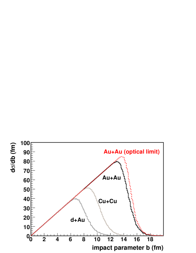
Figure 15: Total geometrical cross section from Glauber Monte Carlo calculations (d+Au, Cu+Cu, and Au+Au at $\sqrt{s_{\mathrm{NN}}}=200$ GeV). The dashed line represents an optical limit calculation for Au+Au.

The total geometric cross section for the collision of two nuclei A and B, i.e., the integral of the distributions $\mathrm{d}\sigma/\mathrm{d}b$ shown in Figure 15, is a basic quantity which can be easily calculated in the Glauber Monte Carlo approach. It corresponds to all Glauber Monte Carlo events with at least one inelastic nucleon-nucleon collision. In ultra-relativistic nucleus-nucleus collisions the de Broglie wave length of the nucleons is small compared to their transverse extent so that quantum mechanical effects are negligible. Hence, the total geometric cross section is expected to be a good approximation of the total inelastic cross section. For the reaction systems in Figure 15 (d+Au, Cu+Cu, and Au+Au at $\sqrt{s_{\mathrm{NN}}}=200$ GeV) the Monte Carlo calculations yield $\sigma_{\mathrm{geo}}^{\mathrm{d+Au}}\approx 2180$ mb, $\sigma_{\mathrm{geo}}^{\mathrm{Cu+Cu}}\approx 3420$ mb, and $\sigma_{\mathrm{geo}}^{\mathrm{Au+Au}}\approx 6840$ mb. The systematic uncertainties are on the order of $10\,\%$ and are dominated by the uncertainties of the nuclear density profile.

Also shown in Figure 15 is a comparison with anf optical calculation of $\mathrm{d}\sigma/\mathrm{d}b$, which shows the effect described in Section 2.3. Optical limit calculations do not naturally contain the terms in the multiple-scattering integral where nucleons “hide” behind each other. This leads to a slightly larger cross section ($\sigma_{\mathrm{geo,optical}}^{\mathrm{Au+Au}}\approx 7280$ mb). While this seems like a small perturbation on $\sigma_{\mathrm{geo}}^{\mathrm{A+B}}$, it has a surprisingly large effect on the extraction of $N_{\mathrm{part}}$ and $N_{\mathrm{coll}}$. This does not come from any fundamental change in the mapping of impact parameter onto those variables. Figure 5 shows the mean value of $N_{\mathrm{coll}}$ (upper curve) and $N_{\mathrm{part}}$ (lower curve) as a function of $b$, where it is seen that the two track each other very precisely over a large range in impact parameter, well within the range usually measured by the RHIC experiments. The problem comes in when dividing a sample up into bins in fractional cross section. While it is straightforward to estimate the most central bins, one finds a systematic difference of $N_{\mathrm{part}}$ between the two calculations as the geometry gets more peripheral.

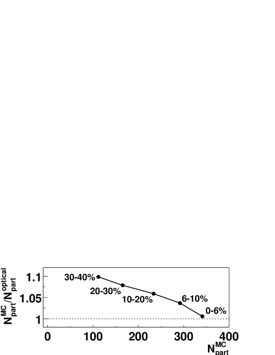
Figure 16: The ratio of $N_{\mathrm{part}}$ calculated with a Glauber Monte Carlo ($N^{\mathrm{MC}}_{\mathrm{part}}$) to that calculated with an optical approximation ($N^{\mathrm{optical}}_{\mathrm{part}}$), for the same fraction of the total inelastic Au+Au cross section ($\sqrt{s_{\mathrm{NN}}}=130$ GeV), plotted as a function of $N^{\mathrm{MC}}_{\mathrm{part}}$ [60].

This is shown in Figure 16 for $\sqrt{s_{\mathrm{NN}}}=130$ GeV by comparing the Monte Carlo calculation in HIJING with the optical limit calculation in [42].

3.4.2 Participants ($N_{\mathrm{part}}$) and Binary Collisions ($N_{\mathrm{coll}}$)

As described in Section 2, the Glauber model is a multiple collision model which treats a nucleus-nucleus (A+B) collision as an independent sequence of nucleon-nucleon collisions. A participating nucleon or wounded nucleon is defined as a nucleon which undergoes at least one inelastic nucleon-nucleon collision. The centrality of a A+B collision can be characterized both by the number of participating nucleons ($N_{\mathrm{part}}$) and by the number of binary nucleon-nucleon collisions ($N_{\mathrm{coll}}$). The average number of participants $\langle N_{\mathrm{part}}\rangle$ and nucleon-nucleon collisions $\langle N_{\mathrm{coll}}\rangle$ as a function of the the impact parameter $b$ are shown in

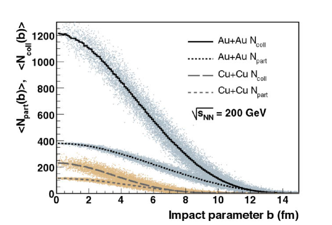
Figure 17: Average number of participants ($\langle N_{\mathrm{part}}\rangle$) and binary nucleon-nucleon collisions ($\langle N_{\mathrm{coll}}\rangle$) along with event-by-event fluctuation of these quantities in the Glauber Monte Carlo calculation as a function of the impact parameter $b$.

Figure 17 for Au+Au and Cu+Cu collisions at $\sqrt{s_{\mathrm{NN}}}=200$ GeV. The event-by-event fluctuations of these quantities for a fixed impact parameter are illustrated by the scatter plots.

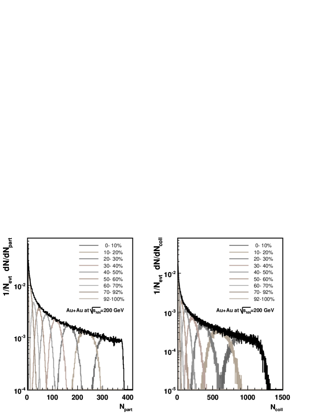
Figure 18: $N_{\mathrm{part}}$ and $N_{\mathrm{coll}}$ distribution in Au+Au collisions at $\sqrt{s_{\mathrm{NN}}}=200$ GeV from a Glauber Monte Carlo calculation. By applying cuts on simulated centrality variables, in this case the BBC and ZDC signal as measured by PHENIX, one obtains $N_{\mathrm{part}}$ and $N_{\mathrm{coll}}$ distributions for the respective centrality class.

The shapes of the $N_{\mathrm{part}}$ and $N_{\mathrm{coll}}$ distributions shown in Figure 18 for Au+Au collisions reflect the fact that peripheral nucleus-nucleus collisions are more likely than central collisions. $\langle N_{\mathrm{part}}\rangle$ and $\langle N_{\mathrm{coll}}\rangle$ for a given experimental centrality class, e.g., the 10% most central collisions, depend on the fluctuations of the centrality variable which is closely related to the geometrical acceptance of the respective detector. By simulating the fluctuations of the experimental centrality variable and applying similar centrality cuts as in the analysis of real data one obtains $N_{\mathrm{part}}$ and $N_{\mathrm{coll}}$ distribution for each centrality class. For peripheral classes the bias introduced by the inefficiency of the experimental minimum bias trigger needs to be taken into account by applying a corresponding trigger threshold on the Glauber Monte Carlo events. Experimental observables like particle multiplicities can then be plotted as a function of the mean value of $N_{\mathrm{part}}$ and $N_{\mathrm{coll}}$ distributions.

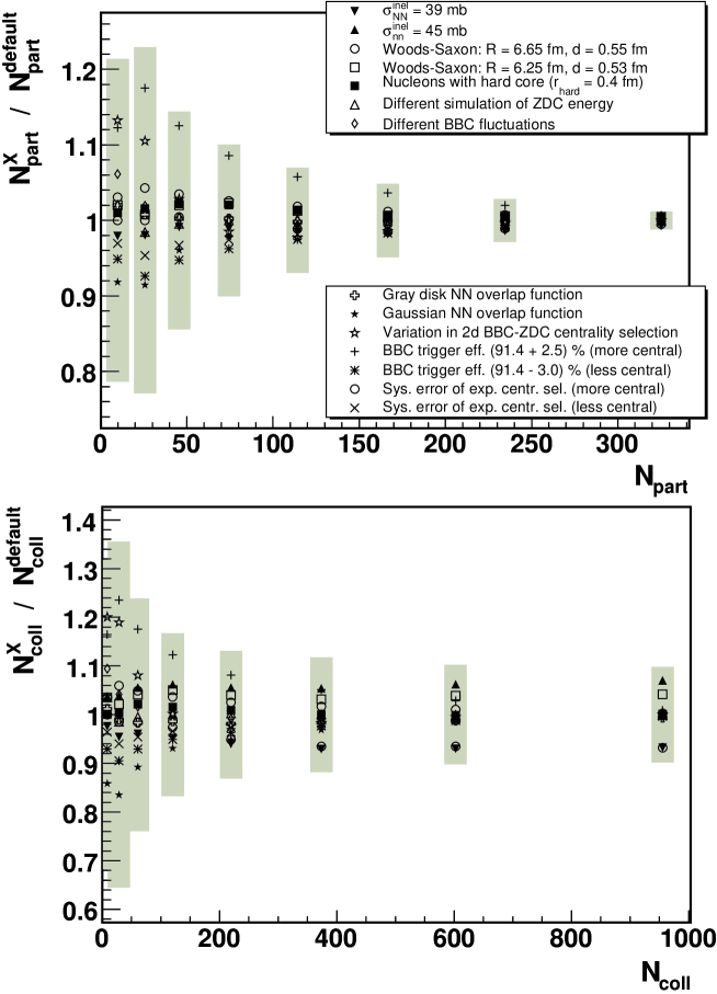
Figure 19: Effect of various parameters in the Glauber Monte Carlo calculation on $N_{\mathrm{part}}$ and $N_{\mathrm{coll}}$ for Au+Au collisions at $\sqrt{s_{\mathrm{NN}}}=200$ GeV.

The systematic uncertainties of $N_{\mathrm{part}}$, $N_{\mathrm{coll}}$, and other calculated quantities are estimated by varying various model parameters. Figure 19 shows such a study for Au+Au collisions at $\sqrt{s_{\mathrm{NN}}}=200$ GeV (PHENIX). The following effects were considered:

• The default value of the nucleon-nucleon cross section of $\sigma_{\mathrm{NN}}=42$ mb was changed to 39 mb and 45 mb.

• Woods-Saxon parameters were varied to determine uncertainties related to the nuclear density profile.

• Effects of a nucleon hard core were studied by requiring a minimum distance of 0.8 fm between two nucleons of the same nucleus without distorting the radial density profile.

• Parameters of the BBC and ZDC simulation (e.g. parameters describing the finite resolution of these detectors) were varied.

• The black disk nucleon-nucleon overlap function was replaced by “gray disk” and Gaussian overlap function [31] without changing the total inelastic nucleon-nucleon cross-section.

• The origin of the centrality cuts applied in the scatter plot of ZDC vs. BBC space was modified in the Glauber calculation.

• The uncertainty of the efficiency of the minimum bias trigger leads to uncertainties as to which percentile of the total inelastic cross section actually is selected with certain centrality cuts. The centrality cuts applied on the centrality observable simulated with the Glauber MC were varied accordingly to study the influence on $\langle N_{\mathrm{part}}\rangle$ and $\langle N_{\mathrm{coll}}\rangle$.

• Even if the minimum bias trigger efficiency were precisely known potential instabilities of the centrality detectors could lead to uncertainties as to which percentile of the total cross section is selected. This has been studied by comparing the number of events in each experimental centrality class for different run periods. The effect on $\langle N_{\mathrm{part}}\rangle$ and $\langle N_{\mathrm{coll}}\rangle$ was again studied by varying the cuts on the simulated centrality variable accordingly.

The total systematic uncertainty indicated by the shaded boxes in Figure 19 were obtained by adding the deviations from the default result for each of the items in the above list in quadrature. The uncertainty of $N_{\mathrm{part}}$ decreases from $\sim 20\,\%$ in peripheral collisions to $\sim 3\,\%$ in central Au+Au collisions. $N_{\mathrm{coll}}$ has similar uncertainties as $N_{\mathrm{part}}$ for peripheral Au+Au collisions. For $N_{\mathrm{part}}>100$ (or $N_{\mathrm{coll}}>200$) the relative systematic uncertainty of $N_{\mathrm{coll}}$ remains constant at about $\sim 10\,\%$. Similar estimates for the systematic uncertainties of $N_{\mathrm{part}}$ and $N_{\mathrm{coll}}$ at the CERN SPS energy of $\sqrt{s_{\mathrm{NN}}}=17.2$ GeV were reported in [55].

For the comparison of observables related to hard processes in A+A and p+p collisions it is advantageous to introduce the nuclear overlap function $\langle T_{\mathrm{AB}}\rangle_{\mathrm{f}}$ for a certain centrality class f (see section 4.2) which is calculated in the Glauber Monte Carlo approach as

$$\langle T_{\mathrm{AB}}\rangle_{\mathrm{f}}=\langle N_{\mathrm{coll}}\rangle_{\mathrm{f}}/\sigma_{\mathrm{inel}}^{\mathrm{NN}}\,.$$ (16)

The uncertainty of the inelastic nucleon-nucleon cross section $\sigma_{\mathrm{inel}}^{\mathrm{NN}}$ doesn’t contribute to the systematic uncertainty. Apart from this $\langle T_{\mathrm{AB}}\rangle_{\mathrm{f}}$ has the same systematics uncertainties as $\langle N_{\mathrm{coll}}\rangle_{\mathrm{f}}$.

3.4.3 Eccentricity

One of the surprising features of the RHIC data was the strong event-by-event asymmetries in the azimuthal distributions. This has been attributed to the phenomenon of “elliptic flow”, the transformation of spatial asymmetries into momentum asymmetries by means of hydrodynamic evolution. For any hydrodynamic model to be appropriate, the system must be sufficiently opaque (where opacity is the product of density times interaction cross section) such that the system equilibrates locally at early times. This suggests that the relevant geometric quantity for controlling elliptic flow is the “shape” of the overlap region, which sets the scale for the gradients that develop.

The typical variable used to quantify this shape is the “eccentricity”, defined as

$$\epsilon=\frac{\langle Y^{2}-X^{2}\rangle}{\langle Y^{2}+X^{2}\rangle}\,.$$ (17)

Just as with other variables discussed here, there are two ways to calculate this. In the optical limit, one performs the averages at a fixed impact parameter, weighting by either the local participant or binary collision density. In the Monte Carlo approach, one simply calculates the moments of the participants themselves. Furthermore, one can calculate these moments with the $X$ axis oriented in two natural frames. The first is along the nominal reaction plane (estimated using spectator nucleons). The second is along the short principal axis of the participant distribution itself [56]. The only mathematical difference between the two definitions involves the incorporation of the correlation coefficient $\langle XY\rangle$:

$$\epsilon_{\mathrm{part}}=\frac{\sqrt{(\sigma^{2}_{x}-\sigma^{2}_{y})^{2}+4(\sigma^{2}_{xy})^{2}}}{\sigma^{2}_{x}-\sigma^{2}_{y}}$$ (18)

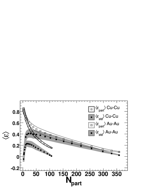
Figure 20: Calculation of eccentricity in Au+Au and Cu+Cu collisions as a function of $N_{\mathrm{part}}$. Both standard and participant eccentricity are shown.

A comparison of the two definitions is shown in Figure 20. One sees very different limiting behavior at very large and small impact parameter. At large impact parameter, fluctuations due to small numbers of participants drive $\epsilon_{\mathrm{std}}\rightarrow 0$, but $\epsilon_{\mathrm{part}}\rightarrow 1$. As $b=0$, $\epsilon_{\mathrm{std}}$ also goes to zero as the system becomes radially symmetric while $\epsilon_{\mathrm{part}}$ now picks up the fluctuations and remains finite. The relevance of these two quantities to actual data will be discussed in sections 4.3 and 4.4.

4 Geometric aspects of p+A and A+A phenomena

4.1 Inclusive Charged-Particle Yields (total and mid-rapidity)

The total multiplicity in hadronic reactions is a measure of the degrees of freedom released in the collision. In the 1970s it was found that the total number of particles produced in proton-nucleus ($p+A$) collisions was proportional to the number of participants, i.e. $N_{\mathrm{ch}}\propto N_{\mathrm{part}}=\nu+1$, where $\nu$ is defined as the number of struck nucleons in the nucleus [61]. This experimental fact was instrumental in establishing $N_{\mathrm{part}}$ as a fundamental physical variable. The situation became more interesting when the total multiplicity was measured in Au+Au at 4 RHIC energies, spanning an order of magnitude in $\sqrt{s_{\mathrm{NN}}}$, and was found to be approximately proportional to $N_{\mathrm{part}}$ there as well.

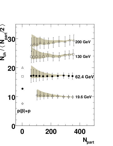
Figure 21: Total inclusive charged-particle multiplicity ($N_{\mathrm{ch}}$) divided by $N_{\mathrm{part}}/2$ from PHOBOS data at four RHIC energies. The data is compared with $p+p$ data or interpolations to unmeasured energies at $N_{\mathrm{part}}=2$.

This is shown in Fig.21 with PHOBOS data from Refs. [58, 59] and is striking if one considers the variety of physics processes that should contribute to the total multiplicity.

By contrast, the inclusive charged-particle density near mid-rapidity ($dN/d\eta(|\eta|<1)$) does not scale linearly with $N_{\mathrm{part}}/2$.

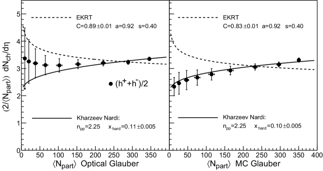
Figure 22: Inclusive charged particle multiplicity near midrapidity ($dN/d\eta(|\eta|<1)$) divided by the number of participating nucleon pairs ($N_{\mathrm{part}}/2$) estimated using the optical approximation (left) and a Glauber Monte Carlo (right) from STAR. The data is compared with two-component fits and a calculation based on parton saturation.

This is shown in Fig. 22 with STAR data, with $N_{\mathrm{part}}$ estimated both from an optical calculation (left) as well as a Glauber Monte Carlo (right) [62]. The comparison shows why care must be taken in the estimation of $N_{\mathrm{part}}$, since using one or the other gives better agreement with very different models. The saturation model of Eskola et al [63] does show scaling with $N_{\mathrm{part}}$ and agrees with the data if $N_{\mathrm{part}}$ is estimated with an optical calculation. However, it disagrees with the data when the GMC approach is used. Better agreement with the data can be found with a so-called “two component” model, e.g. Ref. [42]:

$$\frac{dN}{d\eta}=n_{pp}\left[(1-x)N_{\mathrm{part}}+xN_{\mathrm{coll}}\right]$$ (19)

This model can be fit to the data by a judicious choice of $x$, the parameter which controls the admixture of “hard” particle production. However there is no evidence of any energy dependence to this parameter [65, 64] from $\sqrt{s_{NN}}=$ 19.6 to 200 GeV, suggesting that the source of this dependence has little to nothing to do with hard or semi-hard processes at all.

4.2 Hard Scattering: $T_{\mathrm{AB}}$ Scaling

The number of hard processes between point-like constituents of the nucleons in a nucleus-nucleus collision is proportional to the nuclear overlap function $T_{\mathrm{AB}}(b)$ [66, 67, 68, 69, 70, 71]. This follows directly from the factorization theorem in the theoretical description of hard interactions within perturbative QCD [72]. In detail, the average yield for a hard process with cross section $\sigma_{\mathrm{hard}}^{\mathrm{pp}}$ in p+p collisions per encounter of two nuclei A and B with impact parameter $b$ is given by

$$N_{\mathrm{hard}}^{\mathrm{A+B,enc}}(b)=T_{\mathrm{AB}}(b)\,\sigma_{\mathrm{hard}}^{\mathrm{pp}}\,.$$ (20)

Here $T_{\mathrm{AB}}(b)$ is normalized so that $\int T_{\mathrm{AB}}(b)\,\mathrm{d}^{2}b=AB$. $\sigma_{\mathrm{hard}}^{\mathrm{pp}}$ can, e.g., represent the cross-section for the production of charm-anticharm quark-pairs ($\bar{c}c$) or high-$p_{\mathrm{T}}$ direct photons in proton-proton collisions.

At large impact parameter not every encounter of two nuclei A and B leads to an inelastic collision. Hence, the average number of hard processes per inelastic A+B collision is given by

$$N_{\mathrm{hard}}^{\mathrm{A+B}}(b)=\frac{T_{\mathrm{AB}}(b)}{p_{\mathrm{inel}}^{\mathrm{A+B}}(b)}\cdot\sigma_{\mathrm{hard}}$$ (21)

where $p_{\mathrm{inel}}^{\mathrm{A+B}}(b)$ is the probability of an inelastic A+B collision. In the optical limit $p_{\mathrm{inel}}^{\mathrm{A+B}}(b)$ is given by (cf. Eq. 5)

$$p_{\mathrm{inel}}^{\mathrm{A+B}}(b)=1-\left(1-\sigma_{\mathrm{inel}}^{\mathrm{NN}}\frac{T_{\mathrm{AB}}(b)}{AB}\right)^{AB}\,.$$ (22)

Particle yields at RHIC are usually measured as a function of the transverse momentum ($p_{\mathrm{T}}$). If an invariant cross section $\mathrm{d}\sigma^{\mathrm{pp}}/\mathrm{d}p_{\mathrm{T}}$ for a hard scattering process which leads to the production of a certain particle $x$ has been measured in p+p collisions, then according to Eq. 21 the invariant multiplicity of $x$ per inelastic A+B collisions with impact parameter $b$ is given by

$$\frac{1}{N_{\mathrm{inel}}^{\mathrm{AB}}}\frac{\mathrm{d}N_{x}^{\mathrm{A+B}}}{\mathrm{d}p_{\mathrm{T}}}=\frac{T_{\mathrm{AB}}(b)}{p_{\mathrm{inel}}^{\mathrm{A+B}}(b)}\;\cdot\;\frac{\mathrm{d}\sigma_{x}^{\mathrm{pp}}}{\mathrm{d}p_{\mathrm{T}}}\,.$$ (23)

This baseline expectation is purely based on nuclear geometry and assumes the absence of any nuclear effects. In reality one needs to average over a certain impact parameter distribution. As an example we consider a centrality class f which corresponds to a fixed impact parameter range $b_{1}\leq b\leq b_{2}$. Taking the average in this range over the impact parameter distribution (weighting factor $\mathrm{d}\sigma^{\mathrm{AB}}/\mathrm{d}b=2\pi bp_{\mathrm{inel}}^{\mathrm{A+B}}(b)$) leads to

$$\left.\frac{1}{N_{\mathrm{inel}}^{\mathrm{AB}}}\frac{\mathrm{d}N_{x}^{\mathrm{A+B}}}{\mathrm{d}p_{\mathrm{T}}}\right|_{\mathrm{f}}=\langle T_{\mathrm{AB}}\rangle_{\mathrm{f}}\;\cdot\;\frac{\mathrm{d}\sigma_{x}^{\mathrm{pp}}}{\mathrm{d}p_{\mathrm{T}}}$$ (24)

with

$$\langle T_{\mathrm{AB}}\rangle_{\mathrm{f}}=\frac{\int_{\mathrm{f}}\mathrm{d}^{2}b\,T_{\mathrm{AB}}(b)}{\int_{\mathrm{f}}\mathrm{d}^{2}b\,p_{\mathrm{inel}}^{\mathrm{A+B}}(b)}=\frac{\int\limits_{b_{1}}^{b_{2}}\mathrm{d}b\,2\pi b\,T_{\mathrm{AB}}(b)}{\int\limits_{b_{1}}^{b_{2}}\mathrm{d}b\,2\pi b\,p_{\mathrm{inel}}^{\mathrm{A+B}}(b)}\,.$$ (25)

Averaging over the full impact parameter range ($b_{1}=0$, $b_{2}=\infty$) yields $\langle T_{\mathrm{AB}}\rangle_{\mathrm{f}}=AB/\sigma_{\mathrm{geo}}^{A+B}$. In the Glauber Monte Carlo approach $\langle T_{\mathrm{AB}}\rangle_{\mathrm{f}}$ for a certain centrality class is calculated as

$$\langle T_{\mathrm{AB}}\rangle_{\mathrm{f}}=\langle N_{\mathrm{coll}}\rangle_{\mathrm{f}}/\sigma_{\mathrm{inel}}^{\mathrm{NN}}$$ (26)

where the averaging is done for all A+B collisions with at least one inelastic nucleon-nucleon collision and whose simulated centrality variable belongs to centrality class f.

In order to quantify nuclear effects on particles production in hard scattering processes the nuclear modification factor $R_{\mathrm{AB}}(p_{\mathrm{T}})$ is defined as

$$R_{\mathrm{AB}}(p_{\mathrm{T}})=\frac{(N_{\mathrm{inel}}^{\mathrm{AB}})^{-1}\,\mathrm{d}N_{x}^{\mathrm{A+B}}/\mathrm{d}p_{\mathrm{T}}}{\langle T_{\mathrm{AB}}\rangle_{\mathrm{f}}\,\mathrm{d}\sigma_{x}^{\mathrm{pp}}/\mathrm{d}p_{\mathrm{T}}}\,.$$ (27)

At high $p_{\mathrm{T}}$ ($p_{\mathrm{T}}\geq 2-3$ GeV/$c$ for hadrons and $p_{\mathrm{T}}\geq 4-6$ GeV/$c$ for direct photons) particle production is expected to be dominated by hard processes such that, in the absence of nuclear effects, $R_{\mathrm{AB}}$ should be unity. Due to their electromagnetic nature high-$p_{\mathrm{T}}$ direct photons are essentially unaffected by the hot and dense medium produced in a nucleus-nucleus collisions so that they should exhibit $T_{\mathrm{AB}}$ scaling.

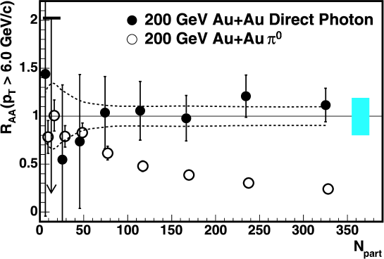
Figure 23: Nuclear modification factor $R_{\mathrm{AA}}$ in Au+Au collisions at $\sqrt{s_{\mathrm{NN}}}=200$ GeV for direct-photon and neutral-pion yields integrated above $p_{\mathrm{T}}=6$ GeV/$c$. The dashed lines indicate the systematic uncertainties of $\langle T_{\mathrm{AB}}\rangle_{\mathrm{f}}$ used in the calculation of $R_{\mathrm{AA}}$.

Fig. 23 shows the nuclear modification factor for direct-photon and neutral-pion yields integrated above $p_{\mathrm{T}}=6$ GeV/$c$ as a function of $N_{\mathrm{part}}$ [73]. Direct photons indeed follow $T_{\mathrm{AB}}$ scaling over the entire centrality range whereas neutral pions are strongly suppressed in central collisions. This is one of the major discoveries at RHIC. The direct-photon measurement is an experimental proof of $T_{\mathrm{AB}}$ scaling of hard processes in nucleus-nucleus collisions. With this observation the most natural explanation for the suppression of high-$p_{\mathrm{T}}$ neutral pions is energy loss of partons from hard scattering in a quark-gluon plasma (jet-quenching) [5, 6, 7, 8].

4.3 Eccentricity and relation to Elliptic Flow

Hydrodynamic calculations suggest that spatial asymmetries in the initial state are mapped directly into asymmetries in the final state momentum distribution. At mid-rapidity, these asymmetries are manifest in the azimuthal ($\phi$) distributions of inclusive and identified charged particles, with the modulation of $\mathrm{d}N/\mathrm{d}\phi\sim 1+2v_{2}\cos[2(\phi-\Psi_{R})]$ characterized by the $2^{nd}$ Fourier coefficient $v_{2}$, where $\Psi_{R}$ defines the angle of the reaction plane for a given event. It is generally assumed that $v_{2}$ is proportional to the event eccentricity $\epsilon$, which was introduced previously. Glauber calculations are used to estimate the eccentricity, either for an ensemble of events or on an event-by-event basis.

For much of the RHIC program, both calculations were typically carried out in the “standard” reference frame, with the X-axis oriented along the reaction plane. Using this calculation method was apparently sufficient to compare hydrodynamic calculations with Au+Au data. However, it was always noticed that the most central events, which should trend to $\epsilon=0$ tended to have a significant $v_{2}$ value. This led to the study of the “participant eccentricity”, calculated with the X axis oriented along the short principal axis of the approximately-elliptical distribution of participants in a Monte Carlo approach [56], described above.

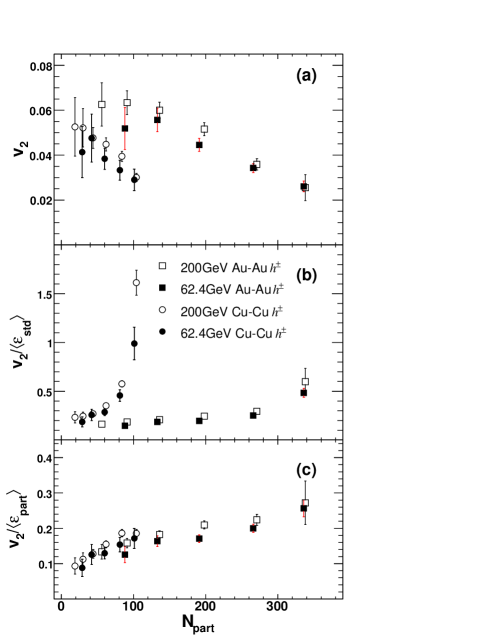
Figure 24: (a) PHOBOS Measurements of $v_{2}$ for 62.4 and 200 GeV Cu+Cu and Au+Au collisions (four system/energy combinations in all, from Ref. [74]), (b) $v_{2}$ divided by standard eccentricity and (c) $v_{2}$ divided by participant eccentricity, showing an approximate scaling for all the system/energy combinations.

Fig. 24 from Ref. [74] shows $v_{2}$, the second Fourier coefficient ($\langle\cos(2[\phi-\Psi_{R}])\rangle$) of the inclusive particle yield relative to the estimated reaction plane angle, as a function of $N_{\mathrm{part}}$. In hydrodynamic models, $v_{2}$ is proportional to the eccentricity, suggesting that $v_{2}/\epsilon$ should be a scaling variable. While the raw values of $v_{2}$ as a function of $N_{\mathrm{part}}$ peak at similar levels in Au+Au and Cu+Cu, it is found that dividing by the standard eccentricity makes the two data sets diverge. However, dividing by $\epsilon_{\mathrm{part}}$ shows that the two systems have similar $v_{2}/\epsilon_{\mathrm{part}}$ at the same $N_{\mathrm{part}}$. This shows that the participant eccentricity, a quantity calculated in a simple Glauber Monte Carlo approach, drives the hydrodynamic evolution of the system for very different energy and geometries.

4.4 Eccentricity Fluctuations

As described above, one of the most spectacular measurements at RHIC was the large value of elliptic flow in Au+Au collisions, suggestive of a “Perfect Liquid.” After the initial measurement [75], much attention was given to potential biases that could artificially inflate the extraction of $v_{2}$ from the data, such as “non-flow” effects (e.g., correlations from jet fragmentation, resonance decay) and event-by-event fluctuations in $v_{2}$ itself. Reference [32] was one of the first analyses to study the effects of fluctuations on extraction of $v_{2}$. Using the assumption $v_{2}\sim\epsilon_{\mathrm{std}}$, fluctuations in $\epsilon_{\mathrm{std}}$ were studied using a Monte Carlo Glauber calculation and comparing $\langle\epsilon_{\mathrm{std}}^{n}\rangle$ to $\langle\epsilon_{\mathrm{std}}\rangle^{n}$. Fluctuations were found to play a significant role, where different methods of extraction (e.g. 2-particle vs. higher order cumulants) gave results differing by as much as a factor of two, with the most significant differences found for the most central (0-5%) and most peripheral (60-80%) events classes.

Recently in references [53] and [76], the STAR and PHOBOS collaborations have reported measurements of not only the $\langle v_{2}\rangle$, but also the r.m.s. width $\sigma_{v_{2}}$.

$\begin{array}[]{c@{\hspace{0.05in}}c}\lx@intercol\mbox{\bf}\hfil\lx@intercol&\lx@intercol\mbox{\bf}\hfil\lx@intercol\\[-15.07993pt] \epsfbox{data_vs_b.eps}\hfil\hfil\hskip 3.61371pt&\epsfbox{finalresultwithEccPart.eps}\hfil\\[-5.69046pt] \mbox{\bf(a)}\hfil\hskip 3.61371pt&\mbox{\bf(b)}\end{array}$

Figure 25: (a) Elliptic flow mean value (top) and r.m.s. width scaled by the mean (bottom) as measured by STAR, compared to various dynamical models and a Monte Carlo Glauber calculation [53]. (b) Gaussian width of $v_{2}$ divided by mean $v_{2}$ from PHOBOS [76].

Figure 25 shows the distribution of $\sigma_{v_{2}}/\langle v_{2}\rangle$ vs $\langle b\rangle$ from Au+Au data. The measurements are compared to calculations from various dynamical models as well as Monte Carlo Glauber calculations using both $\sigma_{\epsilon_{\mathrm{std}}}/\langle\epsilon_{\mathrm{std}}\rangle$ and $\sigma_{\epsilon_{\mathrm{part}}}/\langle\epsilon_{\mathrm{part}}\rangle$. Clearly the $\epsilon_{\mathrm{std}}$ description is ruled out while the $\epsilon_{\mathrm{part}}$ description is in good agreement within the measured uncertainties, implying that the measurements are sensitive to the initial conditions. The agreement with the $\epsilon_{\mathrm{part}}$ Glauber calculation further implies that the measured $v_{2}$ fluctuations are fully accounted for by the fluctuations in the initial geometry, leaving little room for other sources (e.g., Color Glass Condensate). We note that these analyses are new and the physics conclusions are far from final. However, this is another excellent example where Glauber calculations are critical in interpreting RHIC data.

4.5 $J/\psi$ absorption in normal nuclear matter

Due to the large mass of the charm quark $c\bar{c}$ pairs are expected to be produced only in hard processes in the initial phase of a nucleus-nucleus collision. The production rate for $c\bar{c}$ pairs is thus calculable within perturbative QCD which makes them a calibrated probe of later stages of a heavy ion collision. In particular, it was suggested that free color charges in a quark-gluon plasma could prevent the formation of a $J/\psi$ from the initially produced $c\bar{c}$ pairs so that $J/\psi$ suppression was initially considered a key signature of a QGP formation [77]. However, a suppression of $J/\psi$’s relative to the expected production rate for hard processes was already seen in proton-nucleus (p+A) collisions. Thus, it became clear that the “conventional” $J/\psi$ suppression in p+A collisions needed to be quantified and extrapolated to A+B collisions before any conclusions could be drawn about a possible QGP formation in A+B collisions. Cold nuclear matter effects which affect $J/\psi$ production include the modification of the parton distribution in the nucleus (shadowing) and the absorption of pre-resonant $c\bar{c}$ pairs [78]. For the extrapolation of the latter effect from p+A to A+A collisions the Glauber model is frequently used [79], as described in the following.

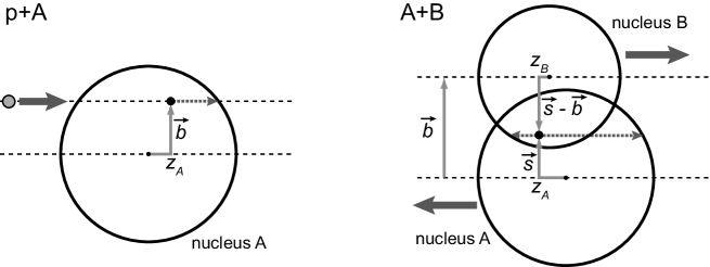
Figure 26: Sketch illustrating the calculation of the $J/\psi$ absorption in normal nuclear matter in proton-nucleus (left panel) and nucleus-nucleus (right panel) collisions). The dashed arrows indicate the paths of a $c\bar{c}$ pair created in a hard process.

We first concentrate on p+A collisions (left panel of Fig. 26). Conventional $J/\psi$ suppression is thought to be related to the path along the $z$ axis in normal nuclear matter a pre-resonant $c\bar{c}$ pair created at point $({\bf b},z_{\mathrm{A}})$ needs to travel. Since the $c\bar{c}$ pair is created in a hard process the location of its production is indeed rather well defined. Usually the effects of processes which inhibit the formation of a $J/\psi$ from the pre-resonant $c\bar{c}$ pair are parameterized with a constant “absorption” cross section $\sigma_{\mathrm{abs}}$. Furthermore, formation time effects are often neglected. Under these assumptions the probability for the break-up of a pre-resonant $c\bar{c}$ state created at $({\bf b},z_{\mathrm{A}})$ in a collision with a certain nucleon $j$ of nucleus A then reads [27, 30]

$$p_{\mathrm{abs}}({\bf b},z_{\mathrm{A}})=\sigma_{\mathrm{abs}}\,\hat{T}_{\mathrm{A>}}({\bf b},z_{\mathrm{A}})\quad\mathrm{with}\quad\hat{T}_{\mathrm{A>}}({\bf b},z_{\mathrm{A}})=\int\limits_{z_{\mathrm{A}}}^{\infty}\hat{\rho}_{\mathrm{A}}({\bf b},z)\,\mathrm{d}z\,.$$ (28)

Here $\hat{\rho}_{\mathrm{A}}$ is the density profile of nucleus A normalized so that integration over full space yields unity. Hence, the total survival probability for the $c\bar{c}$ pair is

$$p_{\mathrm{surv}}^{\mathrm{A}}({\bf b},z_{\mathrm{A}})=\left(1-\sigma_{\mathrm{abs}}\,\hat{T}_{\mathrm{A>}}({\bf b},z_{\mathrm{A}})\right)^{A-1}\approx\exp\left(-(A-1)\,\sigma_{\mathrm{abs}}\,\hat{T}_{\mathrm{A>}}({\bf b},z_{\mathrm{A}})\right)$$ (29)

where the approximation holds for large nuclei $A\gg 1$. The term $A-1$ reflects the fact that the $c\bar{c}$-producing nucleon doesn’t contribute to the absorption. The spatial distribution of the produced $c\bar{c}$ pairs follows $\hat{\rho}_{\mathrm{A}}({\bf b},z)$. Thus, for impact parameter averaged p+A collisions (“minimum bias”) the expression for the $J/\psi$ absorption in the Glauber model reads

$$S_{\mathrm{p+A}}=\frac{\sigma(p+A\rightarrow J/\psi)}{A\cdot\sigma(p+p\rightarrow J/\psi)}=\int\mathrm{d}^{2}b\,\mathrm{d}z_{\mathrm{A}}\,\hat{\rho}_{\mathrm{A}}({\bf b},z_{\mathrm{A}})\,p_{\mathrm{surv}}^{\mathrm{A}}({\bf b},z_{\mathrm{A}})\,.$$ (30)

Fitting the Glauber model expectation to p+A data yields absorption cross-sections on the order of a few mb at CERN SPS energies [80].

As illustrated by the dashed arrows in the right panel of Fig. 26, a $c\bar{c}$ pair created in a collision of two nuclei A and B has to pass through both nuclei. Analogous to Eq. 28 and 29 the $J/\psi$ survival probability for the path in nucleus B can be written as

$$p_{\mathrm{surv}}^{\mathrm{B}}({\bf s}-{\bf b},z_{\mathrm{B}})=\left(1-\sigma_{\mathrm{abs}}\,\hat{T}_{\mathrm{B<}}({\bf s}-{\bf b},z_{\mathrm{B}})\right)^{B-1}\,,\;\hat{T}_{\mathrm{B<}}({\bf s}-{\bf b},z_{\mathrm{B}})=\int\limits_{-\infty}^{z_{\mathrm{B}}}\hat{\rho}_{\mathrm{B}}({\bf s}-{\bf b},z)\,\mathrm{d}z$$ (31)

The spatial $c\bar{c}$ production probability density follows $\hat{\rho}_{\mathrm{A}}({\bf s},z_{\mathrm{A}})\cdot\hat{\rho}_{\mathrm{B}}({\bf s}-{\bf b},z_{\mathrm{B}})$ so that the normal $J/\psi$ suppression as estimated with the Glauber model for A+B collisions with fixed impact parameter $b$ is given by

$$\frac{\mathrm{d}S_{\mathrm{A+B}}}{\mathrm{d}^{2}b}(b) = \frac{1}{A\,B\,\sigma(p+p\rightarrow J/\psi)}\cdot\frac{\mathrm{d}\sigma(AB\rightarrow J/\psi)}{\mathrm{d}^{2}b}$$

$$= \int\mathrm{d}^{2}s\,\mathrm{d}z_{\mathrm{A}}\,\mathrm{d}z_{\mathrm{B}}\,\hat{\rho}_{\mathrm{A}}({\bf s},z_{\mathrm{A}})\hat{\rho}_{\mathrm{B}}({\bf s}-{\bf b},z_{\mathrm{B}})\;p_{\mathrm{surv}}^{\mathrm{A}}({\bf s},z_{\mathrm{A}})p_{\mathrm{surv}}^{\mathrm{B}}({\bf s}-{\bf b},z_{\mathrm{B}})$$

Here $\mathrm{d}S_{\mathrm{A+B}}/\mathrm{d}^{2}b$ is normalized so that $\int\mathrm{d}^{2}b\,\mathrm{d}S_{\mathrm{A+B}}(b)/\mathrm{d}^{2}b=1$ for $\sigma_{\mathrm{abs}}=0$. Sometimes the $J/\psi$ suppression observed in p+A collisions is extrapolated to A+B collisions within the Glauber framework by calculating an effective path length $L=L_{\mathrm{A}}+L_{\mathrm{B}}$ so that the expected normal $J/\psi$ suppression can be written as [79, 80, 81]

$$S_{\mathrm{A+B}}=\exp(-L\,\rho_{0}\,\sigma_{\mathrm{abs}})$$ (33)

where $\rho_{0}=0.17$ fm^-1 is the nucleon density in the center of heavy nuclei. At the CERN SPS a suppression stronger than expected from the absorption in cold nuclear matter has been observed in central Pb+Pb collisions [81]. This so-called “anomalous” $J/\psi$ suppression has been discussed as a potential signal for a QGP formation at the CERN SPS energy.

5 Discussion and the Future

The Glauber model as used in ultra-relativistic heavy-ion physics is purely based on nuclear geometry. What is left from its origin as a quantum mechanical multiple scattering theory is the assumption that a nucleus-nucleus collisions can be viewed as sequence of nucleon-nucleon collisions and that individual nucleons travel on straight line trajectories. With the number of participants $N_{\mathrm{part}}$ and the number of binary nucleon-nucleon collisions $N_{\mathrm{coll}}$ the Glauber model introduces quantities which are essentially not measurable. Only the forward energy in fixed-target experiments has a rather direct relation to $N_{\mathrm{part}}$.

The motivation for the use of these rather theoretical quantities is manifold. One of the main reasons for the use of geometry-related quantities like $N_{\mathrm{part}}$ calculated with the Glauber model is the possibility to compare centrality dependent observables measured in different experiments. Moreover, the comparison of different reaction system as a function of geometric quantities often leads to new insights. Basically all experiments calculate $N_{\mathrm{part}}$ and $N_{\mathrm{coll}}$ in a similar way using a Monte Carlo implementation of the Glauber model so that the theoretical bias introduced in the comparisons is typically small. Thus, the Glauber model provides a crucial interface between theory and experiment.

The widespread use of the Glauber model is related to the fact that indeed many aspects of ultra-relativistic nucleus-nucleus collisions can be understood purely based on geometry. A good example is the total charged particle multiplicity which scales as $N_{\mathrm{part}}$ over a wide centrality and center-of-mass energy range. Another example is the anisotropic momentum distribution of low-$p_{\mathrm{T}}$ ($p_{\mathrm{T}}<\sim 2$ GeV/$c$) particles with respect to the reaction plane. This so-called elliptic flow has its origin in the spatial anisotropy of the initial overlap volume in non-central nucleus-nucleus collisions. It is a success of the Glauber model that event-by-event fluctuations of the spatial anisotropy of the overlap zone as calculated in the Monte Carlo approach appear to be relevant for the understanding of the measured elliptic flow. In this way, a precise understanding of the Glauber picture has been of central concern for understanding the matter produced at RHIC as a “near perfect fluid”.

The study of particle production in hard scattering processes is another important field of application for the Glauber model. According to the QCD factorization theorem the only difference between p+p and A+A collisions in the perturbative QCD description in the absence of nuclear effects is the increased parton flux. This corresponds to a scaling of the invariant particle yields with the number of binary nucleon-nucleon collisions ($N_{\mathrm{coll}}$) as calculated with the Glauber model. The scaling of hard processes with $N_{\mathrm{coll}}$ or $T_{\mathrm{AB}}$ was confirmed by the measurement of high-$p_{\mathrm{T}}$ direct photons in Au+Au collisions at RHIC. This supported the interpretation of a deviation from $T_{\mathrm{AB}}$ scaling for neutral pions and other hadrons (high-$p_{\mathrm{T}}$ hadron suppression) as a result of parton energy loss in a quark-gluon plasma.

Future heavy ion experiments, both at RHIC and at the LHC will further push our understanding of nuclear geometry. As RHIC experiments study more complex multiparticle observables, the understanding of fluctuations and correlations even in something as apparently simple as the Glauber Monte Carlo will become a limiting factor in interpreting data. And as the study of high $p_{T}$ phenomena involving light and heavy flavor becomes prominent in the RHIC II era, the understanding of nuclear geometry, both experimentally and theoretically, will limit the experimental systematic errors. At the LHC, the precision of the geometric calculations will be limited by the knowledge of $\sigma^{\mathrm{NN}}_{\mathrm{inel}}$, which should be measured in the first several years of the $p+p$ program. After that, Glauber calculations will be a central part of understanding the baseline physics of heavy ions at the LHC in terms of nuclear geometry. It is hoped that this review will prepare the next generation of relativistic heavy ion physicists for tackling these issues.

6 Acknowledgements

The authors would like to thank our colleagues for illuminating discussions, especially Mark Baker, Andrzej Bialas, Wit Busza, Jamie Dunlop, Roy Glauber, Ulrich Heinz, Constantin Loizides, Steve Manly, Alexander Milov, Dave Morrison, Jamie Nagle, Mike Tannenbaum, and Thomas Ullrich. We would like to thank the Editorial staff of Annual Reviews for their advice and patience. Miller acknowledges the support of the MIT Pappalardo Fellowship in Physics. This work was supported in part by the Office of Nuclear Physics of the U.S. Department of Energy under contracts: DE-AC02-98CH10886, DE-FG03-96ER40981, DE-FG02-94ER40818.

References

- [1] Czyz W, Maximon LC. Annals Phys. 52:59 (1969)
- [2] Glauber, RJ. 1959. In Lectures in Theoretical Physics, ed. WE Brittin and LG Dunham, 1:315. New York: Interscience
- [3] Białas A, Bleszyński M, Czyź W. Acta. Phys. Pol. B 8:389 (1977)
- [4] Back BB, et al. Phys. Rev. Lett. 85:3100 (2000)
- [5] Arsene I, et al. Nucl. Phys. A 757:1 (2005)
- [6] Adcox K, et al. Nucl. Phys. A 757:184 (2005)
- [7] Back BB, et al. Nucl. Phys. A 757:28 (2005)
- [8] Adams J, et al. Nucl. Phys. A 757:102 (2005)
- [9] Adler C, et al. Nucl. Instrum. Meth. A 470:488 (2001)
- [10] Franco V, Glauber RJ. Phys. Rev. 142:1195 (1966)
- [11] Glauber RJ. Phys. Rev. 100:242 (1955)
- [12] Czyz W, Lesniak L. Phys. Lett. B. 24:227 (1967)
- [13] Fishbane PM, Trefil JS. Phys. Rev. Lett. 32:396 (1974)
- [14] Franco V. Phys. Rev. Lett. 32:911 (1974)
- [15] Białas A, Bleszyński M, Czyź W. Nucl. Phys. B 111:461 (1976)
- [16] Glauber RJ. Nucl. Phys. A 774:3 (2006)
- [17] Ludlam TW, Pfoh A, Shor A. HIJET. A MONTE CARLO EVENT GENERATOR FOR P NUCLEUS AND NUCLEUS NUCLEUS COLLISIONS. BNL-51921 (1985)
- [18] Shor A, Longacre RS. Phys. Lett. B 218:100 (1989)
- [19] Wang XN, Gyulassy M, Phys. Rev. D 44:3501 (1991); code HIJING 1.383.
- [20] Werner K. Phys. Lett. B 208:520 (1988)
- [21] Sorge H, Stoecker H, Greiner W. Nucl. Phys. A 498:567C. (1989)
- [22] Collard HR, Elton LRB, Hodstadter R. In Landolt-Börnstein, Numerical Data and Functional Relationships in Science and Technology, Volume 2: Nuclear Radii. Berlin:Springer-Verlag (1967)
- [23] De Jager CW, De Vries H, De Vries C. Atom. Data Nucl. Data Tabl. 36:495 (1987).
- [24] Hulthén L, Sagawara M. Handbuch der Physik 39:1 (1957).
- [25] Hodgson PE. Nuclear Reactions and Nuclear Structure p453, Clarendon Press, Oxford, (1971)
- [26] Adler SS, et al. Phys. Rev. Lett. 91:072303 (2003)
- [27] Wong C-Y. Introduction to High-Energy Heavy-Ion Collisions, pp. 251-263. Singapore: World Scientific. 516 pp. (1994)
- [28] Chauvin J, Bebrun D, Lounis A, Buenerd M. Phys. Rev. C. 83:1970 (1983)
- [29] Wibig T, Sobczynska D. J. Phys. G 24:2037 (1998)
- [30] Kharzeev D, Lourenco C, Nardi M, Satz H. Z. Phys. C 74:307 (1997)
- [31] Pi H. Comput. Phys. Commun. 71:173 (1992)
- [32] Miller M, Snellings R. arXiv:nucl-ex/0312008 (2003)
- [33] Alver B, et al. Phys. Rev. Lett. 96:212301 (2006)
- [34] Guillaud JP, Sobol A. Simulation of diffractive and non-diffractive processes at the LHC energy with the PYTHIA and PHOJET MC event generators. CNRS Tech. Rep. LAPP-EXP 2004-06 (2004)
- [35] Sjostrand T, Mrenna S, Skands P. JHEP 0605:026 (2006)
- [36] Yao YM. et al. J. Phys. G 33:1 (2006)
- [37] Adamczyk M,et al. Nucl. Instrum. Meth. A 499:437 (2003)
- [38] Allen M, et al. Nucl. Instrum. Meth. A 499:549 (2003)
- [39] Back BB, et al. Nucl. Instrum. Meth. A 499:603 (2003)
- [40] Braem A, et al. Nucl. Instrum. Meth. A 499:720 (2003)
- [41] Ansorge RE, et al. Z. Phys. C 43:357 (1989)
- [42] Kharzeev D, Nardi M. Phys. Lett. B 507:121 (2001)
- [43] Adler C, et al. Phys. Rev. Lett. 89:202301 (2002)
- [44] Bearden IG, et al. Phys. Lett. B 523:227 (2001)
- [45] Bearden IG, et al. Phys. Rev. Lett. 88:202301 (2002)
- [46] Arsene I, et al. Phys. Rev. Lett. 94:032301 (2005)
- [47] Lee YK, et al. Nucl. Instrum. Meth. A 516:281 (2004)
- [48] GEANT 3.21, CERN program library. http://wwwasdoc.web.cern.ch/wwwasdoc/geant_html3/geantall.html
- [49] Adler SS, et al. Phys. Rev. C 71:034908 (2005) Erratum Phys. Rev. C 71:049901 (2005)
- [50] Aronson SH, et al. Nucl. Instrum. Meth. A 499:480 (2003)
- [51] Adams J, et al. Phys. Rev. C 70:044901 (2004)
- [52] Adams J, et al. Phys. Rev. Lett. 91:172302 (2003)
- [53] Sorensen P. arXiv:nucl-ex/0612021 (2006)
- [54] Adams J, et al. Phys. Rev. Lett. 91:072304 (2003)
- [55] Aggarwal MM, et al. Eur. Phys. J. C 18:651 (2001)
- [56] Manly S, et al. Nucl. Phys. A 774:523 (2006)
- [57] Back BB, et al. Phys. Rev. Lett. 91:052303 (2003).
- [58] Back BB, et al. Phys. Rev. C 74:021901 (2006).
- [59] Back BB, et al. Phys. Rev. C 74:021902 (2006)
- [60] Back BB, et al. Phys. Rev. C 65:031901 (2002)
- [61] Elias JE, et al. Phys. Rev. Lett. 41:285 (1978)
- [62] Adams, J et al. arXiv:nucl-ex/0311017 (2003)
- [63] Eskola KJ, Kajantie, K, Ruuskanen, PV, Tuominen, K. Nucl. Phys. B 570:379 (2000)
- [64] Back BB, et al. Phys. Rev. C. 70:021902 (2004)
- [65] Back BB, et al. Phys. Rev. C 65:061901 (2002)
- [66] Eskola KJ, Kajantie K, Lindfors J. Nucl. Phys. B 323:37 (1989)
- [67] Eskola KJ, Vogt R, Wang XN. Int. J. Mod. Phys. A 10:3087 (1995)
- [68] Vogt R. Heavy Ion Phys. 9:339 (1999)
- [69] Arleo F, et al. arXiv:hep-ph/0311131 (2003)
- [70] Jacobs P, Wang XN. Prog. Part. Nucl. Phys. 54:443 (2005)
- [71] Tannenbaum MJ. arXiv:nucl-ex/0611008 (2006)
- [72] Owens JF. Rev. Mod. Phys. 59:465 (1987)
- [73] Adler SS, et al. Phys. Rev. Lett. 94:232301 (2005)
- [74] Alver, B et al. arXiv:nucl-ex/0610037 (2006)
- [75] Ackermann KH, et al. Phys. Rev. Lett. 86:402 (2001)
- [76] Loizides C (for the PHOBOS Collaboration). Proceedings of Quark Matter 2006 (2006)
- [77] Matsui T, Satz H. Phys. Lett. B 178:416 (1986)
- [78] Vogt R. Phys. Rept. 310:197 (1999)
- [79] Gerschel C, Hufner J. Ann. Rev. Nucl. Part. Sci. 49:255 (1999)
- [80] Alessandro B, et al. Eur. Phys. J. C 33:31 (2004)
- [81] Alessandro B, et al. Eur. Phys. J. C 39:335 (2005)