Accuracy of Extracted Multipoles from $\gamma^{*}N\rightarrow\Delta$ Data

Abstract

This work evaluates the model dependence of the electric and Coulomb quadrupole amplitudes (E2, C2) in the predominantly M1 (magnetic dipole-quark spin flip) $\gamma^{*}N\rightarrow\Delta$ transition. Both the model-to-model dependence and the intrinsic model uncertainties are evaluated and found to be comparable to each other and no larger than the experimental errors. It is confirmed that the quadrupole amplitudes have been accurately measured indicating significant non-zero angular momentum components in the proton and $\Delta$.

1 Physics Motivation

Experimental confirmation of the presence of non-spherical hadron amplitudes (i.e. d states in quark models or p wave $\pi$-N states) is fundamental and has been the subject of intense experimental and theoretical interest (for reviews see Drechsel and Tiator (2001); Papanicolas (2003); Bernstein (2003)). This effort has focused on the measurement of the electric and Coulomb quadrupole amplitudes (E2, C2) in the predominantly M1 (magnetic dipole-quark spin flip) $\gamma^{*}N\rightarrow\Delta$ transition. Since the proton has spin 1/2, no quadrupole moment can be measured. However, the $\Delta$ has spin 3/2 so the $\gamma^{*}N\rightarrow\Delta$ reaction can be studied for quadrupole amplitudes in the nucleon and $\Delta$. Due to spin and parity conservation in the $\gamma^{*}N(J^{\pi}=1/2^{+})\rightarrow\Delta(J^{\pi}=3/2^{+})$ reaction, only three multipoles can contribute to the transition: the magnetic dipole ($M1$), the electric quadrupole ($E2$), and the Coulomb quadrupole ($C2$) photon absorption multipoles. The corresponding resonant pion production multipoles are $M_{1+}^{3/2}$, $E_{1+}^{3/2}$, and $S_{1+}^{3/2}$. The relative quadrupole to dipole ratios are EMR=Re($E_{1+}^{3/2}/M_{1+}^{3/2}$) and CMR=Re($S_{1+}^{3/2}/M_{1+}^{3/2}$). In the quark model, the non-spherical amplitudes in the nucleon and $\Delta$ are caused by the non-central, tensor interaction between quarks Glashow (1979). However, the magnitudes of this effect for the predicted E2 and C2 amplitudesCapstick and Karl (1990) are at least an order of magnitude too small to explain the experimental results and even the dominant M1 matrix element is $\simeq$ 30% low Bernstein (2003); Capstick and Karl (1990). A likely cause of these dynamical shortcomings is that the quark model does not respect chiral symmetry, whose spontaneous breaking leads to strong emission of virtual pions (Nambu-Goldstone Bosons)Bernstein (2003). These couple to nucleons as $\vec{\sigma}\cdot\vec{p}$ where $\vec{\sigma}$ is the nucleon spin, and $\vec{p}$ is the pion momentum. The coupling is strong in the p wave and mixes in non-zero angular momentum components.

However, the multipoles are not observables and must be extracted from the measured cross sections. The five-fold differential cross section for the $p(\vec{e},e^{\prime}p)\pi^{0}$ reaction is written as five two-fold differential cross sections with an explicit $\phi^{*}$ dependence as Drechsel and Tiator (1992)

$$\frac{d^{5}\sigma}{d\Omega_{f}dE_{f}d\Omega}=\Gamma(\sigma_{T}+\epsilon\sigma_{L}+v_{LT}\sigma_{LT}\cos\phi^{*}+\epsilon\sigma_{TT}\cos 2\phi^{*}+hp_{e}v_{LT^{\prime}}\sigma_{LT^{\prime}}\sin\phi^{*})$$ (1)

where $\epsilon$ is the transverse polarization of the virtual photon, $v_{LT}=\sqrt{2\epsilon(1+\epsilon)}$, $v_{LT^{\prime}}=\sqrt{2\epsilon(1-\epsilon)}$, $\Gamma$ is the virtual photon flux, $\phi^{*}$ is the pion center of mass azimuthal angle with respect to the electron scattering plane, $h$ is the electron helicity, and $p_{e}$ is the magnitude of the electron longitudinal polarization. The virtual photon differential cross sections ($\sigma_{T},\sigma_{L},\sigma_{LT},\sigma_{TT},\sigma_{LT^{\prime}}$) are all functions of the center of mass energy $W$, the four momentum transfer squared $Q^{2}$, and the pion center of mass polar angle $\theta_{\pi q}^{*}$ (measured from the momentum transfer direction). They are bilinear combinations of the multipoles Drechsel and Tiator (1992).

2 Resonant Multipole Fitting

The current experiments Beck et al. (2000); Blanpied et al. (2001); Warren et al. (1998); Mertz et al. (2001); Kunz et al. (2003); Sparveris et al. (2005); Joo et al. (2002); Frolov et al. (1999); Pospischil et al. (2001); Bartsch et al. (2002); Elsner et al. (2006); Stave et al. (2006) do not have sufficient polarization data to perform a model independent multipole analysis and must rely upon models for the non-resonant (background) amplitudes. The standard procedure to extract the multipoles is to use the models to fit the data. Their background terms are unaltered and the three isospin =3/2 resonance multipoles

$$R_{i}^{3/2}=M_{1+}^{3/2},E_{1+}^{3/2},S_{1+}^{3/2}$$ (2)

are fit to the data. Specifically we introduced multiplicative factors, $\lambda(R_{i})$ for the $I=3/2$ multipoles so that the phase, and hence unitarity, is preserved. For the charge channels with a proton target and an outgoing neutral pion (e.g. $\gamma+p\rightarrow\pi^{0}p$):

$$R_{i}(\pi^{0}p)=R_{i}^{1/2}+\frac{2}{3}\lambda(R_{i})R_{i}^{3/2}$$ (3)

where $R_{i}$ represents any of the three photo-pion multipoles $M_{1+},E_{1+},S_{1+}$ for the final charge state or in the isospin 1/2 and 3/2 states.

Three parameter, resonant multipole fits were performed on data taken at $Q^{2}=0.060$ Stave et al. (2006) and $Q^{2}=0.126$ (GeV/c)² Warren et al. (1998); Mertz et al. (2001); Kunz et al. (2003); Sparveris et al. (2005); Stave (2006), one $Q^{2}$ value at a time, using four representative calculations: the phenomenological MAID 2003 Drechsel et al. (1999) and SAIDArndt et al. (2002)models, and the dynamical models of Sato-Lee Sato and Lee (2001) and DMT Kamalov et al. (2001). The fits are presented in terms of $M_{1+}^{3/2}$, EMR = E2/M1 = Re($E_{1+}/M_{1+})$, and CMR = C2/M1 = Re($S_{1+}/M_{1+})$. At least one multipole is expressed in absolute terms rather than as a ratio because some models can give accurate predictions for ratios but not for absolute sizes. Figure 1 shows our new, low $Q^{2}$ data along with several model predictions before and after the three resonant parameter fitting. The convergence is rather significant. Only the data points in the top three plots were included in the fits and yet the parallel cross section as a function of the center of mass energy $W$ converged nicely. Note that since the Sato-Lee model does not include higher resonances, it was not expected to fit the data well at higher $W$ explaining the deviation observed in Fig. 1. Also, as expected, the $\sigma_{LT^{\prime}}$ curves did not converge since this time reversal odd observable Raskin and Donnelly (1989) is primarily sensitive to background amplitudes and the fit is only for resonant amplitudes.

The bottom half of Figure 1 shows the “spherical” calculated curves when the resonant quadrupole amplitudes ($E_{1+}^{3/2}$ in $\sigma_{0}$ and $S_{1+}^{3/2}$ in $\sigma_{TL}$, see Appendix for multipole expansions of the observables) are set equal to zero. The difference between the spherical and full curves shows the sensitivity of these cross sections to the quadrupole amplitudes and demonstrates the basis of the measurement of the $E_{1+}$ and $S_{1+}$ multipoles. The small spread in the spherical curves indicates their sensitivity to the model dependence of the background amplitudes. Figure 2 shows the values for the EMR and CMR for the four models before and after fitting. It is seen that there is a very strong convergence of these values after fitting. We have quoted the average value of these parameters as the measured value and are using the RMS deviation to estimate the model-to-model errorSparveris et al. (2005); Stave et al. (2006) since these four models are sufficiently different to have a reasonable estimate of the present state of model dependence of the multipoles. At the present time the model-to-model and experimental errors are approximately equal.

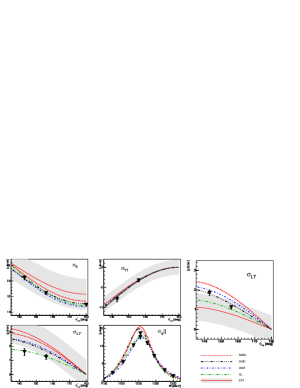
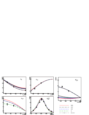
Figure 1: $Q^{2}=0.060$ (GeV/c)² data with model predictions before fitting (top panels) and after the three resonant parameter fit (bottom panels) along with the EFT predictions from Pascalutsa and Venderhaeghen (PV) Pascalutsa and Vanderhaeghen (2005). Note the convergence of the models except for the background sensitive $\sigma_{LT^{\prime}}$ points. Data from Stave et al. (2006) and include the statistical and systematic errors. The lines with dots on them are the fitted models with the $E_{1+}$ and $S_{1+}$ quadrupole terms set to zero. The models are MAID 2003 Drechsel et al. (1999), SAID Arndt et al. (2002), DMT Kamalov et al. (2001) and Sato-Lee (SL) Sato and Lee (2001).

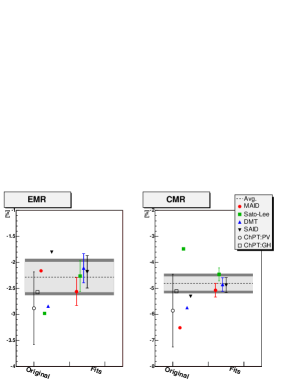
Figure 2: $Q^{2}=0.060$ (GeV/c)² extracted EMR and CMR before and after fitting. The light error band is the average of the fitting errors and the darker band is the RMS deviation of the models added in quadrature. The models are MAID 2003 Drechsel et al. (1999), SAID Arndt et al. (2002), DMT Kamalov et al. (2001) and Sato-Lee Sato and Lee (2001) and the effective field theory calculations of Pascalutsa and Vanderhaeghen (PV) Pascalutsa and Vanderhaeghen (2005) and Gail and Hemmert (GH) Gail and Hemmert (2005). The convergence of the models after fitting is clear.

In a way what we are observing is the fact that the electro-pion production process shows us two separate faces, depending on the observable and on the center of mass energy $W$ that we choose. The best way to extract the three resonant amplitudes is to measure the time reversal even observables ($\sigma_{0},\sigma_{TT},\sigma_{LT}$) Raskin and Donnelly (1989) at or near the resonance energy $W=1232$ MeV. On the other hand, the best way to test the model calculations is to examine time reversal odd observables such as $\sigma_{LT^{\prime}}$ Raskin and Donnelly (1989) right on resonance. In addition, we also have off resonance data. These are sensitive to both the shape and phase of the $M_{1+}$ multipole and also the background amplitudes. The $\gamma p\rightarrow\pi^{+}n$ charge channel is also more sensitive to the background amplitudes particularly the $I=1/2$ amplitudes. Such background sensitive data in combination with model studies are essential if the field is to progress to the stage where the model errors are significantly smaller than the experimental ones.

3 Intrinsic Model Errors in Determination of the Resonant Multipoles

3.1 Beyond Three Parameter Fits: Including Background Multipoles

This work expands the three resonant parameter fits to include the influence of the background multipoles on the resonant amplitudes derived from fitting the experimental data. In this way we will be able to make reasonable estimates of the intrinsic model errors due to uncertainties in the background multipoles and to see if this leads to any suggestions to reduce them. First, we include the remaining s and p wave multipoles: $E_{0+},L_{0+}$, $M_{1-},L_{1-}$. Next, we estimate the influence of the higher partial waves using the CGLN invariant amplitudes $F_{i},i=1,\dots,6$ Drechsel and Tiator (1992). We introduce a new combination of higher order multipoles we call $\overline{F_{i}}$. These combinations show that many small multipoles can have a cumulative effect as will be seen shortly. The $\overline{F_{i}}$s are varied using a scaling factor $\lambda_{i}$ as

$$F_{i} = F_{i}^{S\&P}+\lambda_{i}\overline{F_{i}}$$

$$F_{1} = E_{0+}+3{M_{1+}}\cos\theta+3{E_{1+}}\cos\theta+\lambda_{1}\overline{F_{1}}$$

$$F_{2} = M_{1-}+2{M_{1+}}+\lambda_{2}\overline{F_{2}}$$

$$F_{3} = 3({E_{1+}}-{M_{1+}})+\lambda_{3}\overline{F_{3}}$$

$$F_{4} = \lambda_{4}\overline{F_{4}}$$

$$F_{5} = L_{0+}+6{L_{1+}}\cos\theta+\lambda_{5}\overline{F_{5}}$$

$$F_{6} = L_{1-}-2{L_{1+}}+\lambda_{6}\overline{F_{6}}.$$ (4)

Next, we allow the $I=1/2$ part of the charge channel multipole to vary in a way similar to the $I=3/2$ part.

$$R_{i}(\pi^{0}p)=\lambda(R_{i}^{1/2})R_{i}^{1/2}+\lambda(R_{i})\frac{2}{3}R_{i}^{3/2}.$$ (5)

This new fitting procedure introduces thirteen background amplitudes, too many to determine with the available data. So, we set out to determine how much the resonant parameters are affected by the uncertainties in the background amplitudes. We try to quantify this effect and to determine which parameters have a strong effect and which are correlated.

First, we look for parameters which are correlated with the resonant parameters. Figure 3 shows some examples of negative, positive and no correlation. Fitting parameters are plotted on each axis and the ellipse indicates the region where 68% (1 $\sigma$) of the fits are expected to fall if many similar data sets are fit. The ellipse with axes close to the x and y axes shows no correlation. However, the other ellipses are rotated indicating that as one parameter tends one direction, the other parameter tends to go with it or away from it. This indicates a correlation between the parameters. While error ellipse plots are useful in a qualitative way, they are difficult to use in a quantitative manner. Changes in the scale of the axes will change the angle of the ellipse hiding or exaggerating correlations. Therefore, we use the correlation coefficient, $r$, to indicate the level of correlation between two parameters:

$$r=\frac{\sigma_{12}}{\sigma_{11}\sigma_{22}}$$ (6)

where the error and curvature matrices

$$\left(\begin{array}[]{cc}\epsilon_{11}&\epsilon_{12}\\ \epsilon_{21}&\epsilon_{22}\end{array}\right)^{-1}=\left(\begin{array}[]{cc}\sigma_{11}^{2}&\sigma_{12}\\ \sigma_{21}&\sigma_{22}^{2}\end{array}\right)$$ (7)

are used Eidelman et al. (2004). $r$ varies from -1 to 1 and is insensitive to the parameter scales since the scale factor for each parameter cancels in the ratio. Figure 4 shows the various correlation coefficients for each background amplitude with $E_{1+}^{3/2},M_{1+}^{3/2}$, and $L_{1+}^{3/2}$ using MAID 2003 and combined Bates and Mainz data at $Q^{2}=0.126$ (GeV/c)². The square of $r$ indicates how much of the variance is explained by a linear relation between the two variables. A rule of thumb is that two variables are correlated if $r^{2}\geq 0.5$ and uncorrelated if $r^{2}\leq 0.1$. This then leads to the ranges in $r$: $0.7\leq|r|\leq 1.0=$ large correlation, $0.3\leq|r|<0.7=$ medium correlation, $0.0\leq|r|<0.3=$ small correlation.

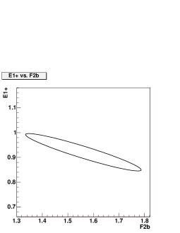
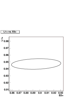
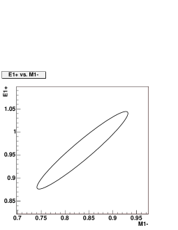
Figure 3: Examples of negative correlation (left), no correlation (center), and positive correlation (right). Note: F2b=$\overline{F_{2}}$.

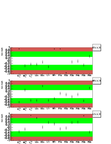
Figure 4: Correlation coefficients for background amplitudes with the resonant amplitudes $E_{1+}^{3/2},M_{1+}^{3/2},L_{1+}^{3/2}$ using MAID 2003 for Mainz and Bates $Q^{2}=0.126$ (GeV/c)² data. The central region of each plot is for small correlation with the next region being medium correlation and the next being large correlation. Note: F1b=$\overline{F_{1}}$, F2b=$\overline{F_{2}}$, etc.

The next check is for sensitivity. If a parameter is large, zeroing it out should affect the $\chi^{2}$ by a large amount. For example, when $L_{0+}$ is turned off, the model predictions change noticeably (see Fig. 5). Other background terms can have significant effects as well like the $\overline{F_{i}}$s and the remaining s and p do in Fig. 6. Table 1 shows the $\chi^{2}$/d.o.f. that results from turning off the various background amplitudes in the MAID 2003 model. It also indicates how strongly the amplitude was correlated with any of the resonant multipoles.

In Figs. 5 and 6, a combined cross sectionPapanicolas (2003); Mertz et al. (2001); Sparveris et al. (2005) $\sigma_{E2}=\sigma_{0}(\theta_{\pi q}^{*})+\sigma_{TT}(\theta_{\pi q}^{*})-\sigma_{0}(\theta_{\pi q}^{*}=\pi)$ is shown. In this linear combination the dominant $M_{1+}$ multipole contribution cancels out and shows the effect of the smaller $E_{1+}$ quadrupole contribution. (See Appendix for the expansion of the observables in terms of multipoles.)

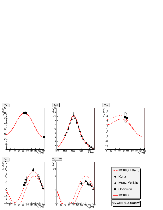
Figure 5: Sensitivity to $L_{0+}$ in MAID 2003 using data at $Q^{2}=0.126$ (GeV/c)². The solid curve is the full MAID 2003 model and the dashed line is with the $L_{0+}$ multipole set to zero. The effect is particularly evident for $\sigma_{LT}$. Data are from Mertz et al. (2001); Kunz et al. (2003); Sparveris et al. (2005) and include statistical, systematic and model errors.

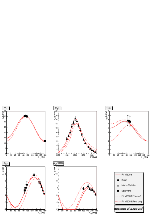
Figure 6: Sensitivity to $\overline{F_{i}}$ and s and p in MAID 2003 using data at $Q^{2}=0.126$ (GeV/c)². As in Fig. 5, the solid curve is the full MAID 2003 while the dashed line is now MAID 2003 with all the $\overline{F_{i}}$s turned off and the dotted line shows the results using only the resonant multipoles. This shows the significant effect the background has on some observables and that the $\overline{F_{i}}$ amplitudes can also have effects of similar size. Data are from Mertz et al. (2001); Kunz et al. (2003); Sparveris et al. (2005) and include statistical, systematic and model errors.

Extra Par.	$\chi^{2}$/d.o.f
$L_{0+}$	7.42
$E_{0+}$	6.09
$\overline{F_{1}}$	5.60
$L_{1+}^{1/2}$	5.59
$M_{1-}$	4.10
$E_{1+}^{1/2}$	3.31
$\overline{F_{5}}$	1.85
$M_{1+}^{1/2}$	1.85
$\overline{F_{2}}$	1.80
$\overline{F_{6}}$	1.72
$L_{1-}$	1.55
$\overline{F_{3}}$	1.24
—	1.21
$\overline{F_{4}}$	1.17

Table 1: Gives $\chi^{2}/$d.o.f. resulting from turning off the corresponding background parameter in MAID 2003 arranged from most to least sensitive using the combined Bates and Mainz $Q^{2}=0.126$ (GeV/c)² data. The type face indicates the level of correlation with any of the three resonant multipoles: Large Correlation Medium or Small Correlation.

Using the criteria of correlation ($|r|>0.7$) and sensitivity ($\chi^{2}$ increases by 50% upon removal), several parameters were identified as significant using the $Q^{2}=0.126$ (GeV/c)² data set. Those multipoles are shown in Table 2 and include two of the s and p multipoles, two of the isospin = 1/2 multipoles and three $\overline{F_{i}}$ terms. Looking at Fig. 7 all seven terms shown in Table 2, when varied, lead to shifted central values or larger error bars for the resonant multipoles. Some, like the $E_{1+}^{1/2}$ with $M_{1+}^{3/2}$ are shifted but not outside the error bars and with no increase in the error bar size and so are not considered significant.

Effort was made to search for a set of criteria using the correlation coefficient and the change in $\chi^{2}$/d.o.f. that would identify all of the parameters which Fig. 7 identifies as significant. The criteria for significance were an increased error and/or a shift in central value. Either indicates a significant effect on the resonant multipole determination. In order to make the criteria robust, other models were put through the selection process as well. In addition to the MAID 2003 model, Sato-Lee, SAID, and DMT were all used. The best identifier of significant parameters turned out to be the single test of $|r|>0.7$. In almost every case, this alone identified all the significant parameters. The $\chi^{2}$ sensitivity would identify some of the sensitive parameters but not others.

E1+	vs.	$E_{1+}^{1/2}$, $M_{1-}$, $\overline{F_{1}}$, $\overline{F_{2}}$
L1+	vs.	$L_{1+}^{1/2}$, $L_{0+}$, $\overline{F_{5}}$

Table 2: Background amplitudes for which the quadrupole amplitudes show sensitivity for MAID 2003 using the criteria listed in the text and the combined Bates and Mainz $Q^{2}=0.126$ (GeV/c)² data.

4 Effect of Background on Resonant Amplitudes

In order to see the effect the sensitive background amplitudes have on the extracted results, the resonant parameters resulting from each four parameter fit were plotted in Fig. 7. The horizontal bar indicates the position and error of the three parameter fit. The background amplitudes identified as significant do have an effect on the extracted multipoles relative to the three parameter fit. For each sensitive background parameter, the error increases and in most cases the central values shift. What is also interesting is that the $\overline{F_{i}}$s have a significant effect. This indicates that many small amplitudes can combine to have a large effect.

To try to quantify the effect of the various background amplitudes on the resonant amplitudes, the RMS deviation of the various four parameter fits was taken for each model and identified as the intrinsic model error. For some fits, the RMS deviation was small and so the average of the four parameter fitting errors was used instead. In both cases, an estimate of the intrinsic error in each model was obtained. The results are shown in Fig. 8 and Table 3 along with the average and RMS deviation of the three parameter fits (model-to-model error). The figure and table indicate that the model-to-model variation is about the same size as the intrinsic model error (specifically for $M_{1+}$ and the CMR the model-to-model error is larger while for the EMR it is somewhat smaller). However, the new error determination procedure is able to use one model alone instead of comparing it with other models. Each models’s error can be assessed independently of the other models.

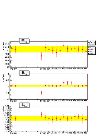
Figure 7: Effect of sensitive parameters on extracted resonance values using MAID 2003 for the combined Mainz and Bates data at $Q^{2}=0.126$ (GeV/c)². Note the larger error bars and shifted central positions of certain combinations of multipoles. The horizontal band indicates the value and error resulting from the three resonant parameter fit. Similar plots were made for the remaining models. Their results are shown in Fig. 8 and Table 3.

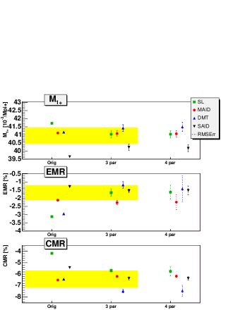
Figure 8: Comparison of the estimated intrinsic and model-to-model errors for all four models at $Q^{2}=0.126$ (GeV/c)², $W=1232$ MeV. The intrinsic error was estimated using the RMS deviation across all the four parameter fits. If the deviation was small, then the average of the four parameter fit errors was used. Cases where the RMS deviation was used are indicated by the dashed vertical error lines. The horizontal band indicates the RMS deviation of the three resonant parameter fits using the four different models.

		3 par. avg.	Model-to-model	Intrinsic errors
			error	MAID	DMT	Sato-Lee	SAID
$M_{1+}$	[$10^{-3}/m_{\pi^{+}}$]	40.94	0.50	0.20	0.29	0.23	0.22
EMR	[%]	-1.65	0.45	0.47	0.78	0.43	0.27
CMR	[%]	-6.43	0.75	0.12	0.47	0.39	0.15

Table 3: Preliminary fitting results and comparison of the estimated intrinsic and model-to-model errors for all four models for the combined Mainz and Bates data at $Q^{2}=0.126$ (GeV/c)², $W=1232$ MeV. See Fig. 8 for calculation details.

While looking to improve the fits, an exhausive search was performed of all combinations of the three resonant parameters and any combination of the 13 remaining parameters. No significant improvement was found for either $Q^{2}=0.060$ or $0.126$ (GeV/c)².

It is time, then, to look beyond fitting the multipoles. It is possible to modify internal model parameters (form factors, coupling constants) which affect many multipoles simultaneously but in different ways. This may allow the models to fit the data better. However, this fitting most likely needs to be performed by the model authors.

The understanding of the $\Delta$ will also be improved with experiments that are closer to complete. With target and recoil polarization, more observables are accessable and these have different combinations of multipoles. These new combinations will further constrain the models allowing better fits and smaller uncertainties in the backgrounds. Until new data are available, though, fitting the data and improving the models remain the best options.

5 Summary and Conclusion

Experimental results using the $\gamma^{*}p\rightarrow p\pi^{0}$ reaction have advanced the understanding of the shape of the proton and the $\Delta$. However, the analysis process begins with extracting multipoles (which are not observables) from cross sections (which are). Without complete experiments including target and recoil polarization, the extraction must rely upon models for the background amplitudes. Performing standard three resonant parameter fits has allowed a good deal of progress to be made. Near resonance, fits using various models converge at $Q^{2}=0.060$ and 0.126 (GeV/c)² despite the differences in the model backgrounds. However, what has not been fully understood is the effect these differing backgrounds can have on the resonant parameters.

To answer that question, we have added thirteen more background amplitudes to our three parameter fits and systematically examined the effect of each one on all three resonant multipoles. Those additional background amplitudes are the four remaining s and p wave amplitudes, three isospin 1/2 amplitudes and six amplitudes we have constructed, the $\overline{F_{i}}$s. The large effect of some of the $\overline{F_{i}}$ terms shows how small multipoles which may have been ignored separately, can combine to have a sizable effect on the resonant amplitudes.

As part of the systematic examination of the additional background amplitudes, correlations were found between them and the resonant amplitudes which led to larger errors and/or shifts in the values of the extracted resonant multipoles. We also found that while some amplitudes exhibit a large sensitivity in $\chi^{2}$, no universal criteria could be found which would predict a sensitivity in the resonant amplitudes. Some background amplitudes which were sensitive did not affect the fits while others which were not sensitive did.

However, varying the background amplitudes which were highly correlated with the resonant multipoles did affect the extracted resonant multipoles. Previous works have shown that the experimental and model-to-model errors are similar in size Stave et al. (2006); Sparveris et al. (2005). What this exercise has shown is that the intrinsic model error is also similar in size to the model-to-model error. The current data really are challenging the existing models. So, without improvement in the models or more complete experiments, this is as far as the current data can take us.

In general, the models agree with the data in a qualitative way but a good quantitative decription will require further refinement of those models. It is possible that some of the models may be made to fit the data much better with adjustment of the proper parameters. Adjusting a form factor or coupling constant within the model will change many multipoles in ways that are different from how they were varied in this study. Once the models are improved, they can be further tested with experiments that utilize target and recoil polarization. These introduce new combinations of multipoles which will further constrain the models. However, until new data are available, improvement of the models is the only option which will allow a better understanding of the $\Delta$.

Finally we return to the question that has primarily motivated this field: Do we have definitive evidence that the nucleon and $\Delta$ have non-spherical components and if so how large? Based on this study we follow reference Papanicolas (2003) and present Figure 9 which indicates the final sensitivity to the quadrupole amplitudes. On the right is $\sigma_{LT}$ which is sensitive to the $S_{1+}$ quadrupole term. On the left is a special construction, $\sigma_{E2}=\sigma_{0}(\theta_{\pi q}^{*})+\sigma_{TT}(\theta_{\pi q}^{*})-\sigma_{0}(\theta_{\pi q}^{*}=\pi)$Papanicolas (2003); Mertz et al. (2001); Sparveris et al. (2005) which cancels out the dominant $M_{1+}$ multipole contribution and shows the effect of the smaller $E_{1+}$ quadrupole contribution. In Fig. 9, the range of predictions using all the four parameter fits was found by cycling through all the fits and storing the maximum and minimum. In this way, a high probability region was identified where the physical multipole would be expected to be. For comparison, the same procedure was repeated but with the quadrupole amplitudes set to zero. On the basis of this study of the uncertainties in the resonance and background amplitudes we agree with the previous conclusionPapanicolas (2003) that a significant contribution of quadrupole amplitudes has been observed.

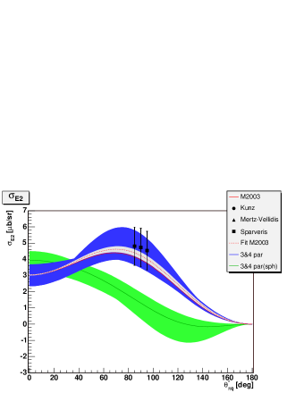
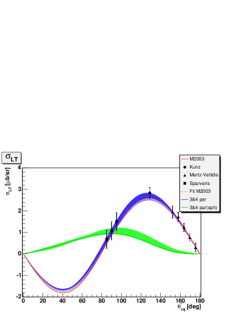
Figure 9: $\sigma_{E2}$ (left) and $\sigma_{LT}$ (right) with error bands showing the range of all the MAID 2003 four parameter fits with (blue/dark region) and without (green/gray region) the quadrupole terms. The data are clearly in the region indicating quadrupole strength similar in size to that found in the models. These plots represent fits using the MAID 2003 model. The light region surrounding the MAID 2003 fit was found using the errors in the three parameter fit with fixed background terms. Data are from Mertz et al. (2001); Kunz et al. (2003); Sparveris et al. (2005) and include statistical, systematic and model errors.

6 Appendix:Contribution of Higher Partial Waves in the Leading Multipole Approximation

The response functions can be expanded keeping only the terms which interfere with the dominant $M_{1+}$ multipole. The multipoles for $L\geq 2$ have been combined into the $\overline{F_{i}}$s in the following expansions which are called the Leading Multipole Approximation (LMA):

$$R_{T}^{LMA} = \left(\frac{5}{2}-\frac{3}{2}\cos^{2}\theta\right)|M_{1+}|^{2}$$ (8)

$$+ 6\cos^{2}\theta{\rm Re}\left[E_{1+}^{*}M_{1+}\right]$$

$$- \sin^{2}\theta\left(3{\rm Re}\left[E_{1+}^{*}M_{1+}\right]+{\rm Re}\left[M_{1+}^{*}\overline{F_{3}}\right]\right)$$

$$+ (1-3\cos^{2}\theta)\left({\rm Re}\left[M_{1+}^{*}M_{1-}\right]+{\rm Re}\left[M_{1+}^{*}\overline{F_{2}}\right]\right)$$

$$+ 2\cos\theta\left({\rm Re}\left[E_{0+}^{*}M_{1+}\right]+{\rm Re}\left[M_{1+}^{*}\overline{F_{1}}\right]\right)$$

$$R_{TT}^{LMA} = -{\rm Re}\left[M_{1+}^{*}(3E_{1+}+3\overline{F_{2}}+\overline{F_{3}}+3M_{1-})\right]\sin^{2}\theta$$ (9)

$$- \frac{3}{2}|M_{1+}|^{2}\sin^{2}\theta$$

$$R_{LT}^{LMA} = \sin\theta{\rm Re}\left[M_{1+}^{*}(\overline{F_{5}}+L_{0+}+6L_{1+}\cos\theta)\right]$$ (10)

$$R_{LT^{\prime}}^{LMA} = \sin\theta{\rm Im}\left[M_{1+}^{*}(\overline{F_{5}}+L_{0+}+6L_{1+}\cos\theta)\right]$$ (11)

$$\sigma_{E2}^{LMA} = -12\sin^{2}\theta{\rm Re}\left[E_{1+}^{*}M_{1+}\right]$$ (12)

$$- 2{\rm Re}\left[M_{1+}^{*}\overline{F_{3}}\right]\sin^{2}\theta$$

$$+ \left(2\cos\theta+2\right)\left({\rm Re}\left[E_{0+}^{*}M_{1+}\right]+{\rm Re}\left[M_{1+}^{*}\overline{F_{1}}\right]\right)$$

References

- Drechsel and Tiator (2001) D. Drechsel, and L. Tiator, editors, Proceedings of the Workshop on the Physics of Excited Nucleons, World Scientific, 2001.
- Papanicolas (2003) C. N. Papanicolas, Eur. Phys. J. A18, 141–145 (2003).
- Bernstein (2003) A. M. Bernstein, Eur. Phys. J. A17, 349–355 (2003).
- Glashow (1979) S. L. Glashow, Physica A96, 27–30 (1979).
- Capstick and Karl (1990) S. Capstick, and G. Karl, Phys. Rev. D41, 2767 (1990).
- Drechsel and Tiator (1992) D. Drechsel, and L. Tiator, J. Phys. G18, 449–497 (1992).
- Beck et al. (2000) R. Beck, et al., Phys. Rev. C61, 035204 (2000).
- Blanpied et al. (2001) G. Blanpied, et al., Phys. Rev. C64, 025203 (2001).
- Warren et al. (1998) G. A. Warren, et al., Phys. Rev. C58, 3722 (1998).
- Mertz et al. (2001) C. Mertz, et al., Phys. Rev. Lett. 86, 2963–2966 (2001).
- Kunz et al. (2003) C. Kunz, et al., Phys. Lett. B564, 21–26 (2003).
- Sparveris et al. (2005) N. F. Sparveris, et al., Phys. Rev. Lett. 94, 022003 (2005).
- Joo et al. (2002) K. Joo, et al., Phys. Rev. Lett. 88, 122001 (2002).
- Frolov et al. (1999) V. V. Frolov, et al., Phys. Rev. Lett. 82, 45–48 (1999).
- Pospischil et al. (2001) T. Pospischil, et al., Phys. Rev. Lett. 86, 2959–2962 (2001).
- Bartsch et al. (2002) P. Bartsch, et al., Phys. Rev. Lett. 88, 142001 (2002).
- Elsner et al. (2006) D. Elsner, et al., Eur. Phys. J. A27, 91–97 (2006).
- Stave et al. (2006) S. Stave, et al. (2006), nucl-ex/0604013.
- Stave (2006) S. Stave, PhD dissertation (unpublished), MIT (2006).
- Drechsel et al. (1999) D. Drechsel, O. Hanstein, S. S. Kamalov, and L. Tiator, Nucl. Phys. A645, 145–174 (1999).
- Arndt et al. (2002) R. A. Arndt, et al., Phys. Rev. C66, 055213 (2002), http://gwdac.phys.gwu.edu.
- Sato and Lee (2001) T. Sato, and T. S. H. Lee, Phys. Rev. C63, 055201 (2001).
- Kamalov et al. (2001) S. S. Kamalov, et al., Phys. Lett. B522, 27–36 (2001).
- Raskin and Donnelly (1989) A. S. Raskin, and T. W. Donnelly, Ann. Phys. 191, 78 (1989).
- Pascalutsa and Vanderhaeghen (2005) V. Pascalutsa, and M. Vanderhaeghen, Phys. Rev. Lett. 95, 232001 (2005).
- Gail and Hemmert (2005) T. A. Gail, and T. R. Hemmert (2005), nucl-th/0512082.
- Eidelman et al. (2004) S. Eidelman, et al., Phys. Lett. B592, 1 (2004).