The QCD transition temperature: results with physical masses in the continuum limit

The transition temperature ($T_{c}$) of QCD is determined by Symanzik improved gauge and stout-link improved staggered fermionic lattice simulations. We use physical masses both for the light quarks ($m_{ud}$) and for the strange quark ($m_{s}$). Four sets of lattice spacings ($N_{t}$=4,6,8 and 10) were used to carry out a continuum extrapolation. It turned out that only $N_{t}$=6,8 and 10 can be used for a controlled extrapolation, $N_{t}$=4 is out of the scaling region. Since the QCD transition is a non-singular cross-over there is no unique $T_{c}$. Thus, different observables lead to different numerical $T_{c}$ values even in the continuum and thermodynamic limit. The peak of the renormalized chiral susceptibility predicts $T_{c}$=151(3)(3) MeV, wheres $T_{c}$-s based on the strange quark number susceptibility and Polyakov loops result in 24(4) MeV and 25(4) MeV larger values, respectively. Another consequence of the cross-over is the non-vanishing width of the peaks even in the thermodynamic limit, which we also determine. These numbers are attempted to be the full result for the $T$$\neq$0 transition, though other lattice fermion formulations (e.g. Wilson) are needed to cross-check them.

1 Introduction

The $T\neq 0$ QCD transition plays an important role in the physics of the early Universe and of heavy ion collisions (most recently at RHIC at BNL; future plans exist for the LHC at CERN and FAIR at GSI). In this letter we study the absolute scales of the transition at vanishing chemical potential ($\mu$=0), which is of direct relevance for the early universe ($\mu$ is negligible there) and for present heavy ion collisions (at RHIC $\mu$$<$$\sim$40 MeV, which is far less than the typical hadronic scale). The transition is known to be a cross-over [1] (at least using staggered fermions, for a discussion about the fourth-root trick, which is usually applied see e.g. [2] and references therein).

There are several results in the literature for $T_{c}$ using both staggered and Wilson fermions [3, 4, 5, 6, 7, 8]. Note however, that these results have typically four serious limitations. a) The first one is related to the unphysical spectrum. b) Another question is how to extrapolate to vanishing lattice spacing (a$\rightarrow$0), approaching the continuum limit. c) The third problem is how to set the absolute scale for a question, which needs an answer of a few percent accuracy. d) Finally the fourth problem is related to some implicit assumptions about a a real singularity, thus ignoring the analytic cross-over feature of the finite temperature QCD transition.

Our goal is to eliminate all these limitations and give the full answer.

ad a. All previous calculations were carried out with unphysical spectra. On the one hand, results with Wilson fermions were obtained with pion masses $m_{\pi}\raise 1.29167pt\hbox{$>$\kern-7.5pt\raise-4.73611pt\hbox{$\sim$}}$560 MeV when approaching the thermodynamical limit (since lattice QCD can give only dimensionless combinations, it is more precise to say that $m_{\pi}$/$m_{\rho}$$>$$\sim$0.7, where $m_{\rho}$ is the mass of the rho meson). The transition is related to the spontaneous breaking of the chiral symmetry (which is driven by the pion sector) and the three physical pions have masses smaller than the transition temperature, thus the numerical value of $T_{c}$ could be sensitive to the unphysical spectrum. Though at $T$=0 chiral perturbation theory provides a technique to extrapolate to physical $m_{\pi}$, no such controllable method exists around $T_{c}$. On the other hand, results with staggered fermions suffer from taste violation. There is one lightest pion state and a large (usually several 100 MeV) unphysical mass splitting between this lightest state and the higher lying other pion states. This mass splitting results in an unphysical spectrum. The artificial pion mass splitting disappears only in the continuum limit. For some choices of the actions the restoration of the proper spectrum happenes only at very small lattice spacings, whereas for other actions somewhat larger lattice spacings are already satisfactory.

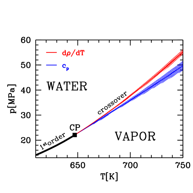
Figure 1: The phase diagram of water around its critical point (CP). For pressures below the critical value ($p_{c}$) the transition is first order, for $p>p_{c}$ values there is a rapid crossover. In the crossover region the critical temperatures defined from different quantities are not necessarily equal. This can be seen for the temperature derivative of the density ($d\rho/dT$) and the specific heat ($c_{p}$). The bands show the experimental uncertainties (see [12]).

Our solution for problem (a) is threefold. First of all, we use physical quark masses in our staggered analysis (or equivalently we fix $m_{K}$/$f_{K}$ and $m_{K}$/$m_{\pi}$ to their experimental values, here $m_{K}$ and $f_{K}$ are the mass and decay constant of the kaon). Secondly, our choice of action (stout link improved fermions) leads to smaller pion mass splittings than other choices (see Fig. 1 of Ref. [9]). The third ingredient is the continuum limit extrapolation which removes the pion mass splitting completely.

ad b. Lattice QCD uses a discretized version of the Lagrangian and approaches the continuum limit by taking smaller and smaller lattice spacings. For lattice spacings which are smaller than some approximate limiting value the dimensionless ratio of different physical quantities have a specific dependence on the lattice spacing (for staggered QCD the continuum value is approached in this region by corrections proportional to the square of the lattice spacing). For these lattice spacings we use the expression: $a^{2}$ scaling region. Clearly, results at least three different lattice spacings are needed to decide, whether one is already in this scaling region or not (two points can always be fitted by $c_{0}$+$c_{2}$$a^{2}$, independently of possible large higher order terms). Only using the $a^{2}$ dependencies in the scaling region, is it possible to unambiguously define the absolute scale of the system. Outside the scaling region different quantities lead to different overall scales, which lead to ambiguous values for e.g. $T_{c}$.

Our solution for problem (b) is straightforward. We approach the scaling region by using four different sets of lattice spacing, which are defined as the transition region on $N_{t}$=4,6,8 and 10 lattices. The results show (not surprisingly) that the coarsest lattice with $N_{t}$=4 is not in the $a^{2}$ scaling region, whereas for the other three a reliable continuum limit extrapolation can be carried out.

ad c. An additional problem appears if we want to give dimensionful predictions with a few percent accuracy. As we already emphasized lattice QCD predicts dimensionless combinations of physical observables. For dimensionful predictions one calculates an experimentally known dimensionful quantity, which is used then to set the overall scale. In many analyses the overall scale is related to some quantities which strictly speaking do not even exist in full QCD (e.g. the mass of the rho eigenstate and the string tension are not well defined due to decay or string breaking). A better, though still not satisfactory possibility is to use quantities, which are well defined, but can not be measured directly in experiments. Such a quantity is the heavy quark-antiquark potential (V), or its characteristic distances: the $r_{0}$ or $r_{1}$ parameters of V [11] ($r^{2}d^{2}V/dr^{2}$=1.65 or 1, for $r_{0}$ or $r_{1}$, respectively). For these quantities intermediate lattice calculations and/or approximations are needed to connect them to measurements. These calculations are based on $\Upsilon$ spectroscopy. This procedure leads to further, unnecessary systematic uncertainties.

The ultimate solution is to use quantities, which can be measured directly in experiments and on the lattice. We use the decay constant of the kaon $f_{K}$=159.8 MeV, which has about 1% measurement error. Detailed additional analyses were done by using the mass of the $K^{*}(892)$ meson $m_{K^{*}}$, the pion decay constant $f_{\pi}$ and the value of $r_{0}$, which all show that we are in the $a^{2}$ scaling regime and our choice of overall scale is unambiguous.

ad d. The QCD transition at non-vanishing temperatures is an analytic cross-over [1]. Since there is no singular temperature dependence different definitions of the transition point lead to different values. The most famous example for this phenomenon is the water-vapor transition, for which the transition temperature can be defined by the peaks of $d\rho/dT$ (temperature derivative of the density) and $c_{p}$ (heat capacity at fixed pressure). For pressures ($p$) somewhat less than $p_{c}=22.064$ MPa the transition is of first order, whereas at $p=p_{c}$ the transition is second order. In both cases the singularity guarantees that both definitions of the transition temperature lead to the same result. For $p>p_{c}$ the transition is a rapid cross-over, for which e.g. both $d\rho/dT$ and $c_{p}$ show pronounced peaks as a function of the temperature, however these peaks are at different temperature values. Figure 1 shows the phase diagram based on [12].

Analogously, there is no unique transition temperature in QCD. Therefore, we determine $T_{c}$ using the sharp changes of the temperature (T) dependence of renormalized dimensionless quantities obtained from the chiral condensate ($\langle\bar{\psi}\psi\rangle$), quark number susceptibility ($n_{q}$) and Polyakov loop ($P$).

The paper is organized as follows. In Section 2 we define our action, discuss the simulation techniques and list our simulation points at T=0, which will be used to carry out our continuum extrapolation procedure unambiguously. Section 3 deals with the different definitions of observables, which are used to locate the transition point at T$\neq$0. Having located the transition in the lattice parameter space we make a connection to dimensionful physical quantities, thus determine the overall scale and carry out the continuum extrapolation. In Section 4 we conclude.

2 Lattice action, simulations at T=0 and setting the scale

In this letter we use a tree-level Symanzik improved gauge, and a stout-improved staggered fermionic action (for the detailed form of our action see eqs. (2.1-2.3) of Ref. [9]). The stout-smearing [13] reduces the taste violation, a lattice artefact of the staggered type of fermions. In a previous study we showed that this sort of smearing has the smallest taste violation among the ones used in the literature for large scale thermodynamical simulations.

We have not improved the high temperature behavior of the fermion action, however due to the order of magnitude smaller costs (compared to e.g. the p4 fat3 action) we could afford to take smaller lattice spacings ($N_{t}=4,6,8$ and $10$). This turned out to be extremely beneficial, when converting the transition temperature into physical units. In particular the $T=0$ simulations -which are used to do this conversion- have very large lattice artefacts at $N_{t}=4$ and $6$ lattice spacings and can not be used for controlled continuum extrapolations. The high-temperature improvement is not designed to reduce these artefacts.

Since we want to determine the transition temperature with high precision, it is important that the quark masses are tuned precisely to their physical values. We have to tune the lattice quark masses along the Line of Constant Physics (LCP) as we are approaching the continuum limit. Using three flavor simulations we already determined a first approximation of the LCP in Ref. [9]. 2+1 flavor simulations with these parameters showed, however, that the hadron mass ratios slightly differ from their physical values. In order to eliminate all uncertainties related to an unphysical spectrum, we determined a new line of constant physics. The new LCP was defined by fixing $m_{K}/f_{K}$ and $m_{K}/m_{\pi}$ to their experimental values (c.f. Figure 1 of [1]).

In order to perform the necessary renormalizations of the measured quantities and to fix the scale in physical units we carried out $T=0$ simulations on our new LCP (c.f. Table 1). Six different $\beta$ values were used. Simulations at T=0 with physical pion masses are quite expensive and in our case unnecessary (chiral perturbation theory provides a controlled approximation at vanishing temperature). Thus, for each $\beta$ value we used four different light quark masses, which resulted in pion masses somewhat larger than the physical one (the $m_{\pi}$ values were approximately 250 MeV, 320 MeV, 380 MeV and 430 MeV), whereas the strange quark mass was fixed by the LCP at each $\beta$. The lattice sizes were chosen to satisfy the $m_{\pi}N_{s}\geq 4$ condition. However, when calculating the systematic uncertainties of meson masses and decay constants, we have taken finite size corrections into account using continuum finite volume chiral perturbation theory [14] (these corrections were around or less than 1%). We have simulated between 700 and 3000 RHMC trajectories for each point in Table 1.

Chiral extrapolation to the physical pion mass led to $m_{K}/f_{K}$ and $m_{K}/m_{\pi}$ values, which agree with the experimental numbers on the 2% level. (Differences resulting from various fitting forms and finite volume corrections were included in the systematics.) This is the accuracy of our LCP.

$\beta$	$m_{s}$	$m_{ud}$	lattice size
$3.330$	0.23847	0.02621	$12^{3}\cdot 24$
		0.04368	$12^{3}\cdot 24$
		0.06115	$12^{3}\cdot 24$
		0.07862	$12^{3}\cdot 24$
$3.450$	0.15730	0.01729	$16^{3}\cdot 32$
		0.02881	$12^{3}\cdot 28$
		0.04033	$12^{3}\cdot 28$
		0.05186	$12^{3}\cdot 28$
$3.550$	0.10234	0.01312	$16^{3}\cdot 32$
		0.01874	$16^{3}\cdot 32$
		0.02624	$12^{3}\cdot 28$
		0.03374	$12^{3}\cdot 28$
$3.670$	0.06331	0.00928	$24^{3}\cdot 32$
		0.01391	$16^{3}\cdot 32$
		0.01739	$16^{3}\cdot 32$
		0.02203	$14^{3}\cdot 32$
$3.750$	0.05025	0.00736	$24^{3}\cdot 32$
		0.01104	$24^{3}\cdot 32$
		0.01473	$16^{3}\cdot 32$
		0.01841	$16^{3}\cdot 32$

Table 1: Lattice parameters and sizes of our zero temperature simulations. The strange quark mass is varied along the LCP as $\beta$ is changed. The light quark masses, listed at each ($\beta$,$m_{s}$) values, correspond approximately to $m_{\pi}$ values of 250 MeV, 320 MeV, 380 MeV and 430 MeV.

In order to be sure that our results are safe from ambiguous determination of the overall scale, and to prove that we are really in the $a^{2}$ scaling region, we carried out a continuum extrapolation for three additional quantities which could be similarly good to set the scale (we normalized them by $f_{K}$, for $f_{K}$ determination in staggered QCD see [15]). Figure 2 shows the measured values of $m_{K^{*}}/f_{K}$, $f_{\pi}/f_{K}$ and $r_{0}f_{K}$, at different lattice spacings and their continuum extrapolation. Our three continuum predictions are in complete agreement with the experimental results (note, that $r_{0}$ can not be measured directly in experiments; in this case the original experimental input is the spectrum of the $\Upsilon$ resonance, which was used by the MILC, HPQCD and UKQCD collaborations to calculate $r_{0}$ on the lattice [15, 16]).

It is important to emphasize that at lattice spacings given by $N_{t}$=4 and 6 the overall scales determined by $f_{K}$ and $r_{0}$ are differing by $\sim$20-30%, which is most probably true for any other staggered formulation used for thermodynamical calculations. Since the determination of the overall scale has a $\sim$20-30% ambiguity, the value of $T_{c}$ can not be determined with the required accuracy.

For the simulations we were using the RHMC algorithm with multiple time scales [17]. The time consuming parts of the computations were carried out in single precision, however the exact reversibility of the algorithm was achieved. On one of our largest lattices we have cross-checked the results with a fully double precision calculation.

3 T$\neq$0 simulations, transition points for different observables

The T$\neq$0 simulations (c.f. Table 2) were carried out along our LCP (that is at physical strange and light quark masses, which correspond to $m_{K}$=498 MeV and $m_{\pi}$=135 MeV) at four different sets of lattice spacings ($N_{t}=4,6,8$ and $10$) and on three different volumes ($N_{s}/N_{t}$ was ranging between 3 and 6). We have observed moderate finite volume effects on the smallest volumes for quantities which are supposed to depend strongly on light quark masses (e.g.. chiral susceptibility). To determine the transition point we used $N_{s}/N_{t}\geq 4$, for which we did not observe any finite volume effect. The number of RHMC trajectories were between 1500 and 8000 for each parameter set (the integrated autocorrelation time was smaller or around 10 for all our runs).

temporal size ($N_{t}$)	$\beta$ range	spatial sizes ($N_{s}$)
$4$	$3.20-3.50$	$12,16,24$
$6$	$3.45-3.75$	$18,24,32$
$8$	$3.57-3.76$	$24,32,40$
$10$	$3.63-3.86$	$28,40,48$

Table 2: Summary of the T$\neq$0 simulation points.

We considered three quantities to locate the transition point: the chiral susceptibility, the strange quark number susceptibility and the Polyakov-loop. Since the transition at vanishing chemical potential is a cross-over, we expect that all three quantities result in different transition points (similarly to the case of the water, c.f. Figure 1).

Chiral susceptibility

The chiral susceptibility of the light quarks ($\chi$) is defined as

$$\chi_{\bar{\psi}\psi}=\frac{T}{V}\frac{\partial^{2}}{\partial m_{ud}^{2}}\log Z=-\frac{\partial^{2}}{\partial m_{ud}^{2}}f,$$ (1)

where $f$ is the free energy density. Since both the bare quark mass and the free energy density contain divergences, $\chi_{\bar{\psi}\psi}$ has to be renormalized [1].

The renormalized quark mass can be written as $m_{R,ud}=Z_{m}\cdot m_{ud}$. If we apply a mass independent renormalization then we have

$$m_{ud}^{2}\frac{\partial^{2}}{\partial m_{ud}^{2}}=m_{R,ud}^{2}\frac{\partial^{2}}{\partial m_{R,ud}^{2}}.$$ (2)

The free energy has additive, quadratic divergencies. They can be removed by subtracting the free energy at $T=0$ (this is the usual renormalization procedure for the free energy or pressure), which leads to $f_{R}$. Therefore, we have the following identity:

$$m_{ud}^{2}\frac{\partial^{2}}{\partial m_{ud}^{2}}\left(f(T)-f(T=0)\right)=m_{R,ud}^{2}\frac{\partial^{2}}{\partial m_{R,ud}^{2}}f_{R}(T).$$ (3)

the right hand side contains only renormalized quantities, which can be determined by measuring the susceptibilities of the left hand side (for the above expression we use the shorthand notation $m_{ud}^{2}\cdot\Delta\chi_{\bar{\psi}\psi}$). In order to obtain a dimensionless quantity it is natural to normalize the above quantity by $T^{4}$ (which minimizes the final errors). Alternatively, one can use combinations of $T$ and/or $m_{\pi}$ to construct dimensionless quantities (though these conventions lead to larger errors). Since the transition is a cross-over (c.f. discussion d of our Introduction) the maxima of $m_{ud}^{2}/m_{\pi}^{2}\cdot\Delta\chi_{\bar{\psi}\psi}/T^{2}$ or $m_{ud}^{2}/m_{\pi}^{4}\cdot\Delta\chi_{\bar{\psi}\psi}$ give somewhat different values for $T_{c}$.

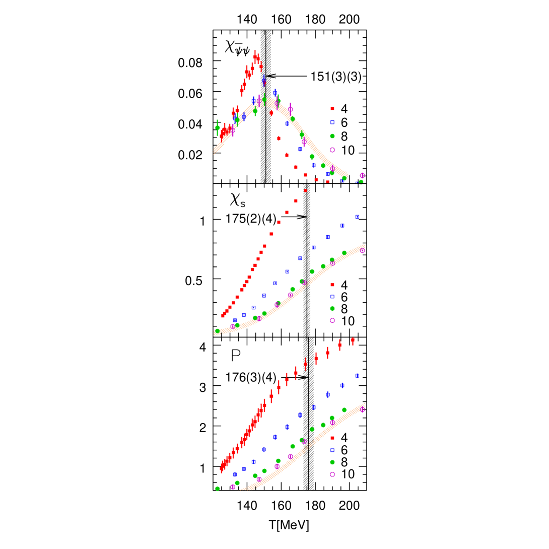
Figure 3: Temperature dependence of the renormalized chiral susceptibility ($m^{2}\Delta\chi_{\bar{\psi}\psi}/T^{4}$), the strange quark number susceptibility ($\chi_{s}/T^{2}$) and the renormalized Polyakov-loop ($P_{R}$) in the transition region. The different symbols show the results for $N_{t}=4,6,8$ and $10$ lattice spacings (filled and empty boxes for $N_{t}=4$ and $6$, filled and open circles for $N_{t}=8$ and $10$). The vertical bands indicate the corresponding critical temperatures and its uncertainties coming from the T$\neq$0 analyses. This error is given by the number in the first parenthesis, whereas the error of the overall scale determination is indicated by the number in the second parenthesis. The orange bands show our continuum limit estimates for the three renormalized quantities as a function of the temperature with their uncertainties.

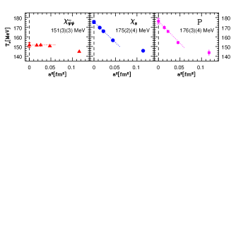
Figure 4: Continuum limit of the transition temperatures obtained from the renormalized chiral susceptibility ($m^{2}\Delta\chi_{\bar{\psi}\psi}/T^{4}$), strange quark number susceptibility ($\chi_{s}/T^{2}$) and renormalized Polyakov-loop ($P_{R}$).

The upper panel of Figure 3 shows the temperature dependence of the renormalized chiral susceptibility for different temporal extensions ($N_{t}$=4,6,8 and 10). For small enough lattice spacings, thus close to the continuum limit, these curves should coincide. As it can be seen, the $N_{t}=4$ result has considerable lattice artefacts, however the two smallest lattice spacings ($N_{t}=8$ and $10$) are already consistent with each other, suggesting that they are also consistent with the continuum limit extrapolation (indicated by the orange band). The curves exhibit pronounced peaks. We define the transition temperatures by the position of these peaks. We fitted a second order expression to the peak to obtain its position. The slight change due to the variation of the fitting range is taken as a systematic error. The left panel of Figure 4 shows the transition temperatures in physical units for different lattice spacings obtained from the chiral susceptibility. As it can be seen $N_{t}$=6,8 and 10 are already in the scaling region, thus a safe continuum extrapolation can be carried out. The extrapolations based on $N_{t}=6,8,10$ fit and $N_{t}=8,10$ fit are consistent with each other. For our final result we use the average of these two fit results (the difference between them are added to our systematic uncertainty). Our T=0 simulations resulted in a $2\%$ error on the overall scale. Our final result for the transition temperature based on the chiral susceptibility reads:

$$T_{c}(\chi_{\bar{\psi}\psi})=151(3)(3){\rm~{}MeV},$$ (4)

where the first error comes from the T$\neq$0, the second from the T=0 analyses.

We use the second derivative of the chiral susceptibility ($\chi^{\prime\prime}$) at the peak position to estimate the width of the peak ($(\Delta T_{c})^{2}=-\chi(T_{c})/\chi^{\prime\prime}(T_{c})$). For the continuum extrapolated width we obtained:

$$\Delta T_{c}(\chi_{\bar{\psi}\psi})=28(5)(1){\rm~{}MeV.}$$ (5)

Note, that for a real phase transition (first or second order), the peak would have a vanishing width (in the thermodynamic limit), yielding a unique value for the critical temperature. Due to the crossover nature of the transition there is no such value, there is a range ($151\pm 28$ MeV) where the transition phenomena takes place. Other quantities than the chiral susceptibility could result in transition temperatures within this range.

The MILC collaboration also reported a continuum result on the transition temperature based on the chiral susceptibility [7]. Their result is 169(12)(4) MeV. Note, that their lattice spacings were not as small as ours (they used $N_{t}$=4,6 and 8), their aspect ratio was quite small ($N_{s}$/$N_{t}$=2), they used non-physical quark masses (their smallest pion mass at T$\neq$0 was $\approx$220 MeV), the non-exact R-algorithm was applied for the simulations and they did not use the renormalized susceptibility, but they looked for the peak in the bare $\chi_{\bar{\psi}\psi}/T^{2}$. Using $T^{4}$ as a normalization prescription (as we did) the transition temperature would decrease their $T_{c}$ values by approximately $9$ MeV. Note, that their continuum extrapolation resulted in a quite large error. Taking into account their uncertainties our result and their result agree on the 1-sigma level.

Quark number susceptibility

For heavy-ion experiments the quark number susceptibilities are quite useful, since they could be related to event-by-event fluctuations. Our second transition temperature is obtained from the strange quark number susceptibility, which is defined via [7]

$$\frac{\chi_{s}}{T^{2}}=\frac{1}{TV}\left.\frac{\partial^{2}\log Z}{\partial\mu_{s}^{2}}\right|_{\mu_{s}=0},$$ (6)

where $\mu_{s}$ is the strange quark chemical potential (in lattice units). Quark number susceptibilities have the convenient property, that they automatically have a proper continuum limit, there is no need for renormalization.

The middle panel of Figure 3 shows the temperature dependence of the strange quark number susceptibility for different temporal extensions ($N_{t}$=4,6,8 and 10). For small enough lattice spacings, thus close to the continuum limit, these curves should coincide again (our continuum limit estimate is indicated by the orange band).

As it can be seen, the $N_{t}=4$ results are quite off, however the two smallest lattice spacings ($N_{t}=8$ and $10$) are already consistent with each other, suggesting that they are also consistent with the continuum limit extrapolation. This feature indicates, that they are closer to the continuum result than our statistical uncertainty.

We defined the transition temperature as the peak in the temperature derivative of the strange quark number susceptibility, that is the inflection point of the susceptibility curve. The position was determined by two independent ways, which yielded the same result. In the first case we fitted a cubic polynomial on the susceptibility curve, while in the second case we determined the temperature derivative numerically from neighboring points and fitted a quadratic expression to the peak. The slight change due to the variation of the fitting range is taken as a systematic error. The middle panel of Figure 4 shows the transition temperatures in physical units for different lattice spacings obtained from the strange quark number susceptibility. As it can be seen $N_{t}$=6,8 and 10 are already in the $a^{2}$ scaling region, thus a safe continuum extrapolation can be carried out. The extrapolations based on $N_{t}=6,8,10$ fit and $N_{t}=8,10$ fit are consistent with each other. For our final result we use the average of these two fit results (the difference between them is added to our systematic uncertainty). The continuum extrapolated value for the transition temperature based on the strange quark number susceptibility is significantly higher than the one from the chiral susceptibility. The difference is 24(4) MeV. For the transition temperature in the continuum limit one gets:

$$T_{c}(\chi_{s})=175(2)(4){\rm~{}MeV},$$ (7)

where the first (second) error is from the T$\neq$0 (T=0) temperature analysis (note, that due to the uncertainty of the overall scale, the difference is more precisely determined than the uncertainties of $T_{c}(\chi_{\bar{\psi}\psi})$ and $T_{c}(\chi_{s})$ would suggest). Similarly to the chiral susceptibility analysis, the curvature at the peak can be used to define a width for the transition.

$$\Delta T_{c}(\chi_{s})=42(4)(1){\rm~{}MeV}.$$ (8)

Polyakov loop

In pure gauge theory the order parameter of the confinement transition is the Polyakov-loop:

$$P=\frac{1}{N_{s}^{3}}\sum_{\bf x}{\rm tr}[U_{4}({\bf x},0)U_{4}({\bf x},1)\dots U_{4}({\bf x},N_{t}-1)].$$ (9)

P acquires a non-vanishing expectation value in the deconfined phase, signaling the spontaneous breakdown of the Z(3) symmetry. When fermions are present in the system, the physical interpretation of the Polyakov-loop expectation value is more complicated (see e.g.. [19]). However, its absolute value can be related to the quark-antiquark free energy at infinite separation:

$$|\langle P\rangle|^{2}=\exp(-\Delta F_{q\bar{q}}(r\to\infty)/T).$$ (10)

$\Delta F_{q\bar{q}}$ is the difference of the free energies of the quark-gluon plasma with and without the quark-antiquark pair.

The absolute value of the Polyakov-loop vanishes in the continuum limit. It needs renormalization. This can be done by renormalizing the free energy of the quark-antiquark pair [20]. Note, that QCD at T$\neq$0 has only the ultraviolet divergencies which are already present at T=0. In order to remove these divergencies at a given lattice spacing we used a simple renormalization condition [21]:

$$V_{R}(r_{0})=0,$$ (11)

where the potential is measured at T=0 from Wilson-loops. The above condition fixes the additive term in the potential at a given lattice spacing. This additive term can be used at the same lattice spacings for the potential obtained from Polyakov loops, or equivalently it can be built in into the definition of the renormalized Polyakov-loop.

$$|\langle P_{R}\rangle|=|\langle P\rangle|\exp(V(r_{0})/(2T)),$$ (12)

where $V(r_{0})$ is the unrenormalized potential obtained from Wilson-loops.

The lower panel of Figure 3 shows the temperature dependence of the renormalized Polyakov-loops for different temporal extensions ($N_{t}$=4,6,8 and 10). The two smallest lattice spacings ($N_{t}=8$ and $10$) are approximately in 1-sigma agreement (our continuum limit estimate is indicated by the orange band).

Similarly to the strange quark susceptibility case we defined the transition temperature as the peak in the temperature derivative of the Polyakov-loop, that is the inflection point of the Polyakov-loop curve. To locate this point and determine its uncertainties we used the same two methods, which were used to determine $T_{c}(\chi_{s})$. The right panel of Figure 4 shows the transition temperatures in physical units for different lattice spacings obtained from the Polyakov-loop. As it can be seen $N_{t}$=6,8 and 10 are already in the scaling region, thus a safe continuum extrapolation can be carried out. The extrapolation and the determination of the systematic error were done as for $T_{c}(\chi_{s})$. The continuum extrapolated value for the transition temperature based on the renormalized Polyakov-loop is significantly higher than the one from the chiral susceptibility. The difference is 25(4) MeV. For the transition temperature in the continuum limit one gets:

$$T_{c}(P)=176(3)(4){\rm~{}MeV},$$ (13)

where the first (second) error is from the T$\neq$0 (T=0) temperature analysis (again, due to the uncertainties of the overall scale, the difference is more precisely determined than the uncertainties of $T_{c}(\chi)$ and $T_{c}(P)$ suggest). Similarly to the chiral susceptibility analysis, the curvature at the peak can be used to define a width for the transition.

$$\Delta T_{c}(P)=38(5)(1){\rm~{}MeV}.$$ (14)

4 Conclusions

We determined the transition temperature of QCD by Symanzik improved gauge and stout-link improved staggered fermionic lattice simulations. We used an exact simulation algorithm and physical masses both for the light quarks and for the strange quark. The parameters were tuned with a quite high precision, thus at all lattice spacings the $m_{K}/f_{k}$ and $m_{k}/m_{\pi}$ ratios were set to their experimental values with an accuracy better than 2%. Four sets of lattice spacings ($N_{t}$=4,6,8 and 10) were used to carry out a continuum extrapolation. It turned out that only $N_{t}$=6,8 and 10 can be used for a controlled extrapolation, $N_{t}$=4 is out of the scaling region. Lattice spacings obtained at the $N_{t}$=6,8 and 10 transition points still result in different values for different physical inputs, but they are already in the scaling region, and an $a^{2}$ type extrapolation can be used. Any extrapolation merely based on $N_{t}$=4 and 6 would contain an unknown systematic error. We demonstrated, that our result is independent of the choice of the physical quantity, which is used to set the overall scale. We calculated three additional quantities, which would give the same dimensionful result for $T_{c}$, since we reproduced their experimental values in the continuum limit. (These ambiguities, related to setting the scale, are serious drawbacks of the analyses which can be found in the literature.)

Since the QCD transition is a non-singular cross-over [1] there is no unique $T_{c}$. We illustrated this well-known phenomenon on the water-vapor phase diagram. Different observables lead to different numerical $T_{c}$ values even in the continuum and thermodynamic limit also in QCD. We used three observables to determine the corresponding transition temperatures. The peak of the renormalized chiral susceptibility predicts $T_{c}$=151(3)(3) MeV, whereas $T_{c}$-s based on the strange quark number susceptibility resulted in 24(4) MeV larger value. Another quantity, which is related to the confining phase transition in the large quark mass limit is the Polyakov loop. Its behavior predicted a 25(4) MeV larger transition temperature, than that of the chiral susceptibility. Another consequence of the cross-over is the non-vanishing widths of the peaks even in the thermodynamic limit, which we also determined. For the chiral susceptibility, strange quark number susceptibility and Polyakov-loop we obtained widths of 28(5)(1) MeV, 42(4)(1) MeV and 38(5)(1) MeV, respectively. These numbers are attempted to be the full result for the $T$$\neq$0 transition, though other lattice fermion formulations (e.g. Wilson) are needed to cross-check them.

Note. After finishing the simulations of the present paper and preparing our manuscript an independent study on $T_{c}$ based on large scale simulations of the Bielefeld-Brookhaven-Columbia-Riken group appeared on the archive [8]. The p4fat3 action was used, which is designed to give very good results in the (T$\longrightarrow$$\infty$) Stefan-Boltzmann limit (their action is not optimized at T=0, which is needed e.g. to set the scale). The overall scale was set by $r_{0}$. The $T_{c}$ analysis based on the chiral susceptibility peak gave in the continuum limit $T_{c}(\chi)$=192(7)(4) MeV. (The second error, 4 MeV, estimates the uncertainty of the continuum limit extrapolation, which we do not use in the following, since we attempt to give a more reliable estimate on that.) This result is in obvious contradiction with our continuum result from the same observable, which is $T_{c}(\chi)$=151(3)(3) MeV. For the same quantity (position of chiral susceptibility peak with physical quark masses in the continuum limit) one should obtain the same numerical result independently of the lattice action. Since the chance probability that we are faced with a statistical fluctuation and both of the results are correct is small, we attempted to understand the origin of the discrepancy. We repeated some of their simulations and analyses. In these cases a complete agreement was found. In addition to their T=0 analyses we carried out an $f_{K}$ determination, too. This $f_{K}$ was used to extend their work, to use an LCP based on $f_{K}$ and to determine $T_{c}$ in physical units.

We summarize the origin of the contradiction between our findings and theirs. The major part of the difference can be explained by the fact, that the lattice spacings of [8] are too large ($>$$\sim$0.20 fm), thus they are not in the $a^{2}$ scaling regime, in which a justified continuum extrapolation could have been done. Setting the scale by different dimensionful quantities should lead to the same result. However at their lattice spacings the overall scales obtained by $r_{0}$ or by $f_{K}$ can differ by $>$$\sim$20%, and even the continuum extrapolated $r_{0}f_{K}$ value of these scales is about 4–5$\sigma$ away from the value given by the literature [15, 16]. This scale ambiguity appears in $T_{c}$, too (though other uncertainties of [8], e.g. coming from the determination of the peak-position, somewhat hide its high statistical significance). We used their $T_{c}$ values fixed by their $r_{0}$ scale, and in addition we converted their peak position of the chiral susceptibility to $T_{c}$ setting the scale by $f_{K}$. (In order to ensure the possibility of a consistent continuum limit –independently of the actual physical value of $r_{0}$– we used for both $r_{0}$ and $f_{K}$ the results of [15, 16] as Ref. [8] did it for $r_{0}$.) Setting the overall scale by $f_{K}$ predicts a much smaller $T_{c}$ at their lattice spacings than doing it by $r_{0}$ (see left panel of Figure 5). Even after carrying out the continuum extrapolation the difference does not vanish ($\sim 30$ MeV), which means that the lattice spacings $>$$\sim$0.20 fm used by [8] are not in the scaling regime. Thus, results obtained with their lattice spacings can not give a consistent continuum limit for $T_{c}$.

In our case not only $N_{t}=4$ and $6$ temporal extensions were used, but more realistic $N_{t}$=8 and $10$ simulations were carried out, which led to smaller lattice spacings. These calculations are already in the $a^{2}$ scaling regime and a safe continuum extrapolation can be done. For our lattice spacing different scale setting methods give consistent results. This is shown on the right panel of Figure 5 (independently of the scale setting one obtains the same $T_{c}$) and also justified with high accuracy by Figure 2, where $r_{0}f_{K}$ converges to the physical value on our finer lattices. As it can be seen on the plot, using only our $N_{t}=4$ and 6 results would also give an inconsistent continuum limit. This emphasizes our conclusion that lattice spacings $>$$\sim$ 0.20 fm can not be used for consistent continuum extrapolations.

The second, minor part of the difference comes from the different definitions of the critical temperatures related to the chiral susceptibility. We use the renormalized chiral susceptibility with $T^{4}$ normalization to obtain the peak position, which yields $\sim 9$ MeV smaller critical temperature than the bare susceptibility normalized by $T^{2}$ of Ref. [8].

Acknowledgment: We thank F. Csikor, J. Kuti and L. Lellouch for useful discussions. We thank P. Petreczky for critical reading of the manuscript. This research was partially supported by OTKA Hungarian Science Grants No. T34980, T37615, M37071, T032501, AT049652, by DFG German Research Grant No. FO 502/1-1 and by the EU Research Grant No. RII3-CT-20040506078. The computations were carried out on the 370 processor PC cluster of Eötvös University, on the 1024 processor PC cluster of Wuppertal University, on the 107 node PC cluster equipped with Graphical Processing Units at Wuppertal University and on the BlueGene/L at FZ Jülich. We used a modified version of the publicly available MILC code [22] with next-neighbor communication architecture for PC-clusters [23].

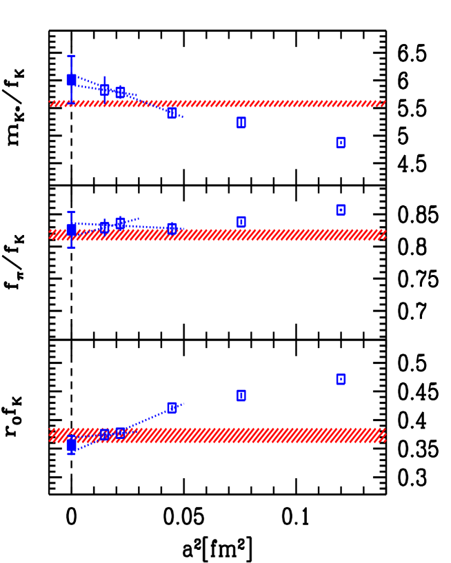
Figure 2: Scaling of the mass of the $K^{*}(892)$ meson, the pion decay constant and $r_{0}$ towards the continuum limit. As a continuum value (filled boxes) we took the average of the continuum extrapolations obtained using our 2 and our 3 finest lattice spacings. The difference was taken as a systematic uncertainty, which is included in the shown errors. The quantities are plotted in units of the kaon decay constant. In case of the upper two panels the bands indicate the physical values of the ratios and their experimental uncertainties. For $r_{0}$ (lowest panel) in the absence of direct experimental results we compare our value with the $r_{0}f_{K}$ obtained by the MILC, HPQCD and UKQCD collaborations [15, 16].

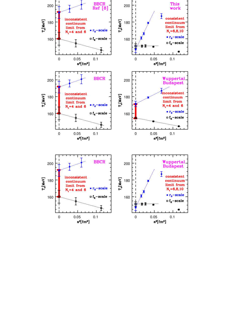
Figure 5: Resolving the discrepancy between the critical temperature of Ref. [8] and that of the present work (see text). The major part of the difference can be traced back to the unreliable continuum extrapolation of [8]. Left panel: In Ref. [8] $r_{0}$ was used for scale setting (filled boxes), however using the kaon decay constant (empty boxes) leads to different critical temperatures even after performing the continuum extrapolation. Right panel: in our work the extrapolations based on the finer lattices are safe, using the two different scale setting methods one obtains consistent results.

References

- [1] Y. Aoki, G. Endrodi, Z. Fodor, S. D. Katz, and K. K. Szabo, The order of the quantum chromodynamics transition predicted by the standard model of particle physics, Nature 443 (2006) 675–678, [hep-lat/0611014].
- [2] C. Bernard, M. Golterman, and Y. Shamir, Observations on staggered fermions at non-zero lattice spacing, Phys. Rev. D73 (2006) 114511 [10 pages], [hep-lat/0604017].
- [3] F. Karsch, E. Laermann, and A. Peikert, Quark mass and flavor dependence of the qcd phase transition, Nucl. Phys. B605 (2001) 579–599, [hep-lat/0012023].
- [4] MILC Collaboration, C. W. Bernard et al., Qcd thermodynamics with an improved lattice action, Phys. Rev. D56 (1997) 5584–5595, [hep-lat/9703003].
- [5] CP-PACS Collaboration, A. Ali Khan et al., Phase structure and critical temperature of two flavor qcd with renormalization group improved gauge action and clover improved wilson quark action, Phys. Rev. D63 (2001) 034502 [11 pages], [hep-lat/0008011].
- [6] DIK Collaboration, V. G. Bornyakov et al., Finite temperature qcd with two flavors of non- perturbatively improved wilson fermions, Phys. Rev. D71 (2005) 114504, [hep-lat/0401014].
- [7] MILC Collaboration, C. Bernard et al., Qcd thermodynamics with three flavors of improved staggered quarks, Phys. Rev. D71 (2005) 034504, [hep-lat/0405029].
- [8] M. Cheng et al., The transition temperature in qcd, hep-lat/0608013.
- [9] Y. Aoki, Z. Fodor, S. D. Katz, and K. K. Szabo, The equation of state in lattice qcd: With physical quark masses towards the continuum limit, JHEP 01 (2006) 089 [16 pages], [hep-lat/0510084].
- [10] S. Naik, On-shell improved lattice action for qcd with susskind fermions and asymptotic freedom scale, Nucl. Phys. B316 (1989) 238.
- [11] R. Sommer, A new way to set the energy scale in lattice gauge theories and its applications to the static force and alpha-s in su(2) yang-mills theory, Nucl. Phys. B411 (1994) 839–854, [hep-lat/9310022].
- [12] B. Spang, http://www.cheresources.com/iapwsif97.shtml, .
- [13] C. Morningstar and M. J. Peardon, Analytic smearing of su(3) link variables in lattice qcd, Phys. Rev. D69 (2004) 054501, [hep-lat/0311018].
- [14] G. Colangelo, S. Durr, and C. Haefeli, Finite volume effects for meson masses and decay constants, Nucl. Phys. B721 (2005) 136–174, [hep-lat/0503014].
- [15] MILC Collaboration, C. Aubin et al., Light pseudoscalar decay constants, quark masses, and low energy constants from three-flavor lattice qcd, Phys. Rev. D70 (2004) 114501, [hep-lat/0407028].
- [16] A. Gray et al., The upsilon spectrum and m(b) from full lattice qcd, Phys. Rev. D72 (2005) 094507, [hep-lat/0507013].
- [17] M. A. Clark and A. D. Kennedy, Accelerating dynamical fermion computations using the rational hybrid monte carlo (rhmc) algorithm with multiple pseudofermion fields, hep-lat/0608015.
- [18] S. D. Katz, Equation of state from lattice qcd, http://qm2005.kfki.hu/talk2_select.pshtml?sel=27.
- [19] S. Kratochvila and P. de Forcrand, Qcd at zero baryon density and the polyakov loop paradox, Phys. Rev. D73 (2006) 114512, [hep-lat/0602005].
- [20] O. Kaczmarek, F. Karsch, P. Petreczky, and F. Zantow, Heavy quark anti-quark free energy and the renormalized polyakov loop, Phys. Lett. B543 (2002) 41–47, [hep-lat/0207002].
- [21] Z. Fodor, S. D. Katz, K. K. Szabo, and A. I. Toth, Grand canonical potential for a static quark anti-quark pair at mu not equal 0, Nucl. Phys. Proc. Suppl. 140 (2005) 508–510, [hep-lat/0410032].
- [22] MILC Collaboration, public lattice gauge theory code, see http://physics.indiana.edu/ sg/milc.html, .
- [23] Z. Fodor, S. D. Katz, and G. Papp, Better than $1/mflops sustained: A scalable pc-based parallel computer for lattice qcd, Comput. Phys. Commun. 152 (2003) 121–134, [hep-lat/0202030].