Mixed Action Simulations on Staggered Background;
Interpretation and Result for the 2-flavor QCD Chiral Condensate

Abstract

Growing evidence indicates that in the continuum limit the rooted staggered action is in the correct QCD universality class, the non-local terms arising from taste breaking can be viewed as lattice artifacts. In this paper we consider the 2–flavor Asqtad staggered action at lattice spacing $a\!\approx\!0.13\,$fm and probe the properties of the staggered configurations by an overlap valence Dirac operator. By comparing the distribution of the overlap eigenmodes to continuum QCD predictions we investigate if/when the lattice artifacts are small as a function of the staggered quark mass. We define a matching overlap quark mass where the lattice corrections are minimal for the topological susceptibility and from the eigenmode distribution we predict the 2–flavor chiral condensate. Our results indicate that the staggered configurations are consistent with 2–flavor continuum QCD up to small lattice artifacts, and predict a consistent value for the infinite volume chiral condensate.

I Introduction

With the advent of improved actions, increasing dedicated computing power, and large scale collaborative efforts, lattice QCD calculations became mainstream, the numerical predictions are often comparable or better than other theoretical calculations. Most of the recent high precision results were obtained using staggered fermions. The 2+1 flavor Asqtad configurations created by the MILC/SciDac collaboration are publicly available and have been used both with staggered valence quarks and also in mixed action simulations with overlap or domain wall fermions.

Staggered fermions are computationally advantageous but the staggered action describes four fermionic flavors. In order to simulate 2+1 flavor QCD the $4^{\mathrm{th}}$ root of the fermionic determinant is taken in the Boltzmann weight. This procedure, usually referred to as rooting, leads to a non-local fermionic action that might not be in the expected 1–flavor QCD universality class. Non-locality does not necessarily mean that the action is incorrect. If the non-local terms are irrelevant, i.e. scale away with the lattice spacing, the staggered action has the correct continuum limit, but this is not automatic and cannot be proven by usual renormalizability arguments Bunk et al. (2004); Adams (2004); Shamir (2005); Hasenfratz (2005); Bernard et al. (2006); Shamir (2006). In Ref. Shamir (2006) Shamir has developed a framework, based on renormalization group considerations, that shows how the non-local terms of the rooted staggered action can become irrelevant. The proof relies on several assumptions, and while those assumptions are quite plausible, their validity has to be checked.

One possibility to support the arguments of Ref. Shamir (2006) and the validity of the rooted staggered action is to numerically verify that the non-local terms become irrelevant in the continuum limit. In a previous work Hasenfratz and Hoffmann (2006a, b) we carried out such a study for the 2–dimensional Schwinger model. We compared the determinant of the staggered lattice action to the determinant of a chiral overlap action with the same flavor number on staggered configuration ensembles. We showed that the difference between the lattice formulations, both local lattice artifacts and non-local terms, scale away with at least $O(a^{2})$ and the continuum limit can be approached with any physical quark mass, even with massless quarks. The result implies that the non-local terms of the rooted action can be considered lattice artifacts when the taste breaking terms of the staggered action are not too large.

In this paper we develop the techniques necessary to carry out a similar study in 4–dimensional QCD. Our approach is different from Ref. Hasenfratz and Hoffmann (2006a) as the high precision evaluation of the fermionic determinant is not feasible in 4 dimensions. Rather we develop a more general method that can be applied to any mixed action simulation.

Mixed action simulations became popular in recent years as they combine the simulation advantages of a simple sea quark action with the exact or near exact chiral symmetry of overlap or domain wall valence quarks. The price to pay, in addition to an internal inconsistency (unitarity violation), is the complication in the analysis. One option is to derive and use partially quenched mixed action chiral perturbative formulae. For staggered sea quarks this approach is particularly cumbersome (although it can be very effective) as the taste breaking terms of the staggered action require the introduction of dozens of parameters in the chiral Lagrangian. It is no longer possible to make physical predictions from individual configuration ensembles, at the end all data enters into the chiral fitter that predicts chirally extrapolated continuum quantities. Another possibility is to match the parameters of the valence and sea quark actions as well as possible and deal with any remaining difference as part of the lattice artifacts. Since the lattice action is characterized by only a few parameters, namely the lattice spacing and the quark masses, this matching is fairly simple. If both the sea and valence actions have small lattice artifacts, their difference after matching should also be small. This latter approach is useful if the chiral perturbative formulae do not exist or the numerical data does not allow the fitting of all the parameters, or if one desires more insight into the physics contained in a particular set of gauge configurations.

The effectiveness of the latter approach was illustrated in Ref. Hasenfratz and Hoffmann (2006a) and while there our main objective was to investigate the validity of the rooting procedure for staggered quarks, we also showed that, at least within the 2–dimensional Schwinger model, mixed action simulations with overlap valance quarks on both 2–flavor (unrooted) and 1–flavor (rooted) staggered sea quark configurations reproduce the full dynamical overlap action results if the overlap mass is tuned appropriately. We illustrated this both for the mass dependence of the topological susceptibility and the (massive) scalar condensate Hasenfratz and Hoffmann (2006b).

In this work we report our first results along the same lines in 4–dimensional 2–flavor QCD. Our strategy is simple: we investigate to what extent configurations generated with rooted staggered fermions describe continuum QCD. The deviation characterizes both local and non-local lattice artifacts. If these terms are irrelevant in the continuum limit, they should scale away as the lattice spacing is decreased at fixed physical quark mass. We do not yet have numerical data to investigate the continuum limit, in this work we concentrate on the mass dependence at fixed lattice spacing. We show that configurations generated with 2–flavor staggered quarks at a single lattice spacing but at four different quark masses are consistent with 2–flavor QCD configurations, at least for the three heavier masses. We also show how the topological charge distributions can be used to determine the best overlap valence matching masses and that with these mass values the data sets predict a consistent value for the chiral condensate of 2–flavor QCD.

In Sect. II we describe our strategy and summarize our numerical setup. The fit of the eigenvalue distributions of the Dirac operator to random matrix theory predictions is discussed in Sect. III, and Sect. IV describes the topological charge distribution. Finally, in Sect. V we combine the previous results to obtain a prediction for the chiral condensate. In this section we also discuss the dependence of the matching valence quark mass on the staggered sea mass.

II Strategy and Simulation setup

We generated configuration sets with the rooted staggered action at fixed lattice spacing and at several quark mass values and ask two very basic questions:

1. Are the staggered configuration sets consistent with $n_{f}\!=\!2$ continuum QCD, up to small lattice artifacts?

2. What is the matching valence overlap quark mass that best describes the staggered configurations?

To investigate the first question one has to consider observables that are sensitive to the vacuum and do not depend strongly on the valence quark mass. Spectral quantities are not appropriate, but the low lying infrared eigenmodes of the massless valence Dirac operator are a good choice. Another quantity, which we will consider, is the topological charge of the configurations.

The answer to the second question is not unique. In fact any “reasonable” choice (i.e. one that approaches the continuum fixed point similarly to the staggered sea quark mass) will work in the continuum limit. However at finite lattice spacing a wise choice of the matching valence mass could significantly reduce lattice artifacts. As it turns out the eigenmodes of the massless Dirac operator are not very sensitive to the sea quark mass but we will be able to use the topological charge distribution to fix the matching valence quark mass.

In our calculation we use an overlap valence quark action, based on an improved Wilson action kernel (planar action) with HYP smeared links Hasenfratz and Knechtli (2001). This is the same action that was used by DeGrand in previous studies DeGrand (2001, 2004).

Our sea quark action is the 2–flavor Asqtad staggered action Orginos et al. (1999); Bernard et al. (2001); Aubin et al. (2004). We have generated four configuration sets, each consisting of 400-500 $12^{4}$ lattices at a lattice spacing of about $a=0.13\,$fm. We have used the Refreshed Molecular Dynamics algorithm from the publicly available MILC code and chose the step size according to Ref. Bernard et al. (2001). The details of the sets are summarized in Table 1. The $\beta=7.2$, $am_{st}=0.02$ (M) set corresponds to the MILC single 2–flavor run.

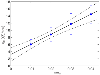
Figure 1: Integrated autocorrelation time of the topological charge vs. staggered quark mass.

The lattice spacing is obtained from the hadronic length scale $r_{0}$ Sommer (1994); Hasenfratz et al. (2002), which we measured on $12^{3}\times 16$ configurations. The values of $r_{0}/a$ are listed in Table 1 together with the simulation parameters. We also quote the level of taste breaking, the ratios of the heaviest and lightest pion masses, approximated from corresponding 2+1 flavor results Bernard et al. (2001). The last column lists the separation of the configurations in terms of unit length molecular dynamics trajectories. These numbers were chosen to reflect the autocorrelation time of the topological charge.

We were surprised to find that the heavier mass data sets had larger autocorrelation times as shown in Fig. 1. We will discuss this problem further at the end of Sect. IV.

Set	$\quad\beta\quad$	$\ am_{st}\$	$\ \ \ r_{0}/a\ \ \ \$	Taste breaking	Time separation
L	7.18	0.01	3.84(6)	60%	5
M	7.20	0.02	3.82(3)	34%	5
H	7.22	0.03	3.60(4)	24%	10
E	7.24	0.04	3.64(3)	18%	15

Table 1: Parameters of the $n_{f}\!=\!2$ staggered background configurations. The taste breaking levels are approximated from corresponding 2+1 flavor runs except for the M set where 2–flavor spectroscopy data exists. The molecular dynamics time separations between the configurations reflect the autocorrelation of the topological charge.

III Eigenvalues of the Dirac Operator and Random Matrix Theory

Random matrix theory (RMT) captures the universal chiral properties of QCD and predicts the distribution of the physical (infrared) eigenvalues of the massless Dirac operator in the $\epsilon$–regime Verbaarschot and Wettig (2000). The predictions are given in fixed topological sector $\nu$ and depend on the low energy constant $\Sigma$, the infinite volume chiral condensate. The distribution of the (microscopically rescaled) $n^{\mathrm{th}}$ eigenmode $\lambda\Sigma V$ is given as

$$P_{\nu,n}(\lambda\Sigma V)=\Lambda_{\nu,n}(m\Sigma V;n_{f})\;,$$ (1)

where $m$ is the sea quark mass and $V$ is the volume of the configurations. $\Lambda_{\nu,n}$ is an $n_{f}$ dependent universal function of the variable $M=m\Sigma V$. While $\Lambda_{\nu,n}$ can in principle be obtained directly from random matrices, analytical forms also exist and are more convenient for evaluating the distribution of the lower modes Damgaard and Nishigaki (2001); Damgaard et al. (2000). While the universal predictions of RMT hold strictly only in the $\epsilon$–regime and in infinite volume, in practice the validity of random matrix theory seems to extend significantly further Giusti et al. (2003); DeGrand (2006).

Since the eigenvalues $\lambda_{\nu,n}$ refer to the massless Dirac operator, the quark mass dependence enters only through the sea quarks. In dynamical simulations, where the same chiral action is used both for the sea and valence sectors, $m$ in Eq.(1) is known and the eigenvalue distribution can be used to predict the chiral condensate $\Sigma$ DeGrand et al. (2006a, b). In our case $m$ is an overlap quark mass that corresponds to the background configurations that were generated by staggered quarks, i.e. $m$ is the matching quark mass as described in Sect. II. The value of $m$ is not known a priori and therefore in our case $P_{\nu,n}(\lambda)$ depends on two variables, $M$ and $\Sigma$. We fit the measured eigenvalue distribution to random matrix theory at fixed $M$ and predict the chiral condensate $\Sigma(M)$. The systematic deviation of the data from the RMT prediction of Eq.(1) characterizes the lattice artifacts, both from discretization errors and from the non-locality of the action. This deviation is the measure of consistency between the lattice action and continuum QCD and replaces the residue used in Ref. Hasenfratz and Hoffmann (2006a) for the same purpose. If the rooting procedure is correct, it should scale to zero as the continuum limit is approached at fixed physical (matching) quark mass, assuming the simulations are done in the region where the RMT predictions are valid.

It is customary to fit the integrated or cumulative eigenvalue distribution, which avoids the binning of the data. The most frequently used fit is the Kolmogorov-Smirnov (KS) test that minimizes $D_{\mathrm{max}}^{2}$, the maximal deviation between the measured and the predicted cumulative distributions Bietenholz et al. (2003); DeGrand et al. (2006a, b).

An advantage of the KS test is that there is an explicit and simple form for the confidence level of the fit that gives the probability that the measured distribution is consistent with the analytical one. This so called quality factor

$$Q_{\mathrm{KS}}(d) = 2\sum_{j=1}^{\infty}(-1)^{j\!+\!1}e^{-2j^{2}d^{2}},$$

$$d = (\sqrt{N}+0.12+0.11/\sqrt{N})D_{\mathrm{max}}$$ (2)

depends on $D_{\mathrm{max}}$ and $N$, the number of configurations in the sample. For our data sets the quality factor is well approximated by the first term in the sum,

$$\log Q_{\mathrm{KS}}\approx\log 2-2ND_{\mathrm{max}}^{2}\;.$$ (3)

The KS fit maximizes the quality factor $Q_{\mathrm{KS}}$ or the product of quality factors if more than one distribution is used. However, $Q_{\mathrm{KS}}$ will go to zero exponentially with increasing statistics if the measured distribution is not exactly described by the analytic form. In any lattice calculation there are lattice artifacts and finite volume effects, so the analytic form is never exactly reproduced, the quality factor vanishes as the numerical statistics increases. Quality factors quoted in this situation are rather meaningless, unless one uses it to compare simulations with identical statistics. On the other hand $D_{\mathrm{max}}$ has a finite limit as the statistics increases and describes the systematic deviation of the numerical and analytical values. In the following we fit our data by maximizing the quality factor (or products of quality factors) according to the KS test but describe the goodness of the fit by the value $D_{\mathrm{max}}$ itself.

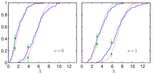
Figure 2: RMT predictions of the cumulative distribution of the two lowest eigenmodes in the $\nu=0$ and $1$ sectors of the M ($am_{st}\!=\!0.02)$ data set at $M\!=\!m\Sigma V\!=\!13.5$ (see below). The fit uses only the first modes of the $\nu=0$ and 1 topological sectors. Arrows indicate the maximal deviation between the data set and the analytical predictions.

The random matrix theory predicts the distribution of the universal, infrared eigenmodes. A rough estimate for the number of such modes comes from the expected number of instantons on each configurations. Since our volume is about 6 fm${}^{4},$ we expect on average 6 instantons per configurations. That implies that only the first 1-2 modes in the $\nu=0-2$ sectors can be expected to be infrared dominated. Somewhat arbitrarily we have decided to fit the first modes in the $\nu=0$ and 1 sectors. Figure 2 shows some typical fits of the cumulative distribution for the M ($am_{st}=0.02)$ data set. The left panel corresponds to the $\nu=0$, the right panel to the $\nu=1$ sector. The first modes of the $\nu=0$ and 1 topological sectors are included in the fit. In addition to the two fitted modes we also show the non-fitted second modes in the same topological sectors. $D_{\mathrm{max}}$ is almost a factor of two smaller for the $n=1$, $\nu=1$ mode, but not significantly worse for the non-fitted modes than for the fitted $n=1$, $\nu=0$ mode.

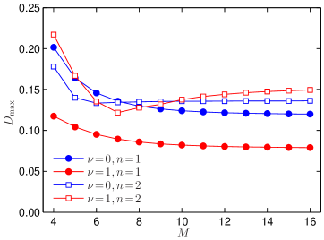
Figure 3: The maximal deviation $D_{\mathrm{max}}$ as the function of $M=m\Sigma V$ for the M data set. The fit is to the first modes of the $\nu=0$ and 1 sectors (filled points). The second modes in the same topological sectors are not fitted (open symbols).

In Fig.3 we plot the maximal deviations $D_{\mathrm{max}}$ as a function of the RMT parameter $M$. Evidently the quality of the fit is not very sensitive to this parameter. While small values are disfavored – $D_{\mathrm{max}}$ increases by a factor of 2 if $M\lesssim 4$ – larger values are almost equally probable. Contrary to our original hopes the eigenmode distributions cannot be used to define a matching mass, it defines only a range of acceptable values. It is interesting to note that the same analysis on the dynamical overlap data set of Ref. DeGrand et al. (2006b) shows a broad but definite minimum in $D_{\mathrm{max}}$ around the actual sea quark mass .

The result of the fit is similar for the other three data sets. The upper panels of Figure 4 show $D_{\mathrm{max}}$ for the fitted modes, and the dependence on the staggered mass is obvious. $D_{\mathrm{max}}$ is significantly lower at the heaviest E data set than for the lightest L one, with the intermediate mass sets lying in between. This behavior is expected since at finite lattice spacing a smaller staggered mass leads to increased taste symmetry breaking (Table 1), it differs more from the flavor symmetric valence quark sector. With decreasing lattice spacing at fixed physical quark mass this deviation should decrease and eventually vanish in the continuum limit.

At each $M=m\Sigma V$ value the fit predicts $\Sigma V/a$. Using the values for $r_{0}/a$ from Table 1 this can be converted to physical units as shown on the lower panels of Fig. 4. The corresponding $am=M/(\Sigma V/a)$ overlap mass values are shown along the upper border of the figure. For those configuration sets that are consistent with continuum QCD the predicted $\Sigma$ values should be identical, independent of the sea quark mass. Unfortunately at this point we do not know the matching $M$ values to predict $\Sigma$. However we can already exclude a simple linear $m=Zm_{st}$ relation with $Z=O(1)$. Such a relation would require that the L and E data sets predict the same condensate at $M$ values that are a factor of 4 different. That is obviously not consistent with the data unless $Z$ is unreasonably large. In order to predict the chiral condensate we have to find an independent quantity that can be used to fix the matching valence quark mass. The topological charge distribution is a possible choice as we will discuss in Sect. IV.

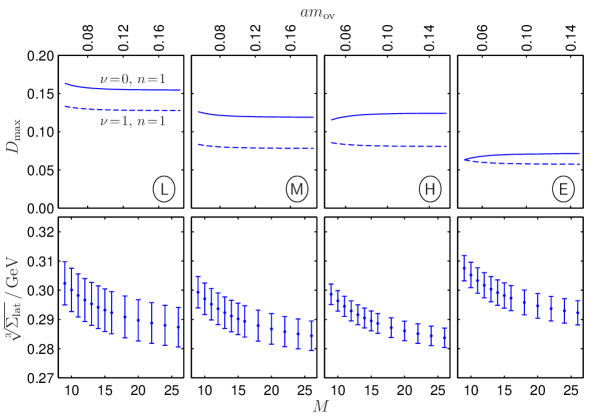
Figure 4: $D_{\mathrm{max}}$ and $\Sigma^{1/3}$ in GeV as the function of $M=m\Sigma V$ for all four data sets.

Set	$\ M=m\Sigma V\$	$\ \Sigma^{1/3}$ / MeV	$am$	$\ \nu\$	$\ N\$	$\ D_{{\rm max}}\$	$\ Q_{{\rm KS}}\$
L	12.7(2.0)	295.7(7.0)	0.083(4)(14)	0	89	0.157	0.022
				1	144	0.130	0.014
M	13.5(2.8)	291.7(4.1)	0.090(3)(19)	0	103	0.121	0.092
				1	172	0.080	0.217
H	16.9(1.9)	288.0(5.4)	0.098(4)(12)	0	87	0.123	0.132
				1	178	0.081	0.181
E	22.6(4.3)	293.5(4.1)	0.127(4)(24)	0	85	0.071	0.768
				1	193	0.058	0.022

Table 2: Results of the RMT fit to the lowest eigenmodes in the $\nu=0,1$ sectors. $N$ is the number of configurations of each data set, $D_{\mathrm{max}}$ is the maximum deviation of the fit and the quality factor $Q_{\mathrm{KS}}$ is defined in Eq. (2). $am$ is the matching overlap mass where the first error is due to the uncertainty of $\Sigma$ only, while the second one takes into account both the errors of $\Sigma$ and $M$. For the determination of $M$ see Sect. IV.

In Table 2 we list the number of configurations we had in the $\nu=0$ and 1 topological sectors, the $D_{\mathrm{max}}$ values of the RMT fit at specific $M=m\Sigma V$ values and the corresponding quality factors. The choice of these $M$ parameters will be explained in Sect. IV. Are these fits and corresponding $D_{\mathrm{max}}$ values reasonable? All our data have been obtained at a single lattice spacing so we cannot investigate the lattice spacing dependence. In order to develop a feel for the quality of the fit we looked at published data both for quenched and dynamical simulations. In Ref. Bietenholz et al. (2003) the $D_{\mathrm{max}}$ values for the first mode on physically slightly smaller $12^{4}$ lattices are 0.27 and 0.08 for $\nu\!=\!0$ and 1, respectively. This study used an improved but not smeared overlap operators on quenched lattices with somewhat smaller lattice spacing than ours. In Ref. DeGrand et al. (2006b) the $D_{\mathrm{max}}$ values of the first non–zero modes using the same fitting strategy as ours are between 0.11 and 0.20. That study used dynamical overlap configurations with the same improved overlap operator we use here with two levels of stout smeared links at a somewhat coarser lattice spacing. In view of these numbers we can conclude that, as far as the Dirac operator eigenmode distribution is concerned, the rooted staggered action configurations do not show larger lattice artifacts than the overlap ones. Even the worst set with the lightest quark mass is comparable to the overlap data.

IV Topology

We have seen in Sect. III that the low energy eigenmodes of the massless overlap Dirac operator are consistent with continuum QCD as predicted by RMT as long as the quantity $M=m\Sigma V$ is larger than some minimal value. The RMT fit however does not restrict $m$ any further. A matching along the lines of Ref. Hasenfratz and Hoffmann (2006a), with the determinants approximated by a small number of infrared modes, can in principle be used to fix the valence quark mass. While this method gives masses in the expected range, the result varies with the number of included modes (we measured 8 overlap and 32 staggered eigenvalues). Unless more eigenmodes are available, this leads to unacceptably large errors in the overlap mass. We therefore need to consider another physical observable in order to match $m$ to the dynamical configurations. Again, we want to use a quantity that is sensitive to the vacuum structure and not the valence quark sector, so we chose the topological charge.

Since we have sufficient statistics, over 400 approximately independent configurations at each coupling value on not too large volumes ($12^{4}$ or about 6 fm⁴), we can study the topological charge distribution. Following the discussion of Refs. Leutwyler and Smilga (1992); Verbaarschot and Wettig (2000); Durr (2001), we write the probability of encountering a charge $\pm\nu$ configuration in the dynamical ensemble as

$$P_{\nu}=Z_{\nu}(m\Sigma V)Q_{\nu}(\sigma)\;.$$ (4)

Here $Q_{\nu}$ is the quenched probability of a charge $\pm\nu$ configuration while $Z_{\nu}$ describes the suppression due to the fermionic determinant. Based on simple probabilistic arguments $Q_{\nu}$ is expected to be a Gaussian distribution. Recent large scale simulations support this expectation in large volumes Giusti et al. (2003). The data is consistent with

$$Q_{\nu}(\sigma)=\frac{1}{\sqrt{2\pi\sigma^{2}}}e^{-\nu^{2}/2\sigma^{2}}\{1+O(V^{-1})\}\;,$$ (5)

where $\sigma^{2}=\langle\nu^{2}\rangle_{Q}=V\chi_{Q}$ is the expectation value of the charge squared in the quenched theory. The fermionic suppression factor has been calculated both within chiral perturbation theory and the random matrix model Leutwyler and Smilga (1992); Verbaarschot and Wettig (2000). For 2 flavors it is

$$Z_{\nu}=I_{\nu}^{2}(M)-I_{\nu-1}(M)I_{\nu+1}(M)\;,$$ (6)

where the $I_{\nu}(M)$ are modified Bessel functions. Thus the charge probability distribution $P_{\nu}$ depends on two variables, $M=m\Sigma V$ and $\sigma$. The latter can be determined from the quenched topological susceptibility, so a one parameter fit to the topological charge distribution data predicts $M$.

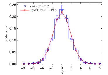
Figure 5: The topological charge distribution for the M data set with fit to Eq.(4).

Figure 5 shows such a fit for the M configuration set using $\chi_{Q}r_{0}^{4}=0.072$ from Ref. Giusti et al. (2003). The fit predicts $M=13.5(2.8)$ with $\chi^{2}/\mathrm{DoF}=0.65$. The predicted $M$ values for the other data sets are listed in Table 2. While the quality of the fit is very similar for the lightest L data set, for heavier masses we encountered difficulties in sampling the topological charge distribution due to long autocorrelation times. Even with increased separation between consecutive configurations the charge distribution does not look Gaussian. Both in the H and E data set the $\nu=0$ sector is under-represented. This probably implies that we still underestimate the autocorrelation time at the larger quark masses. While the topological charge value changes from configuration to configuration and covers both negative and positive values, we have observed systematic shifts from zero average that persist over tens of configurations. This possibly could signal an occasional large topological object that is destroyed only very slowly, but is accompanied by many frequently changing smaller objects. We are not sure if this is the consequence of the inexact R algorithm or similar problems would be encountered in exact molecular dynamics simulations as well. As an illustration Fig. 6 shows the distribution of the topological charge on the E set that contains 550 configurations. In this set we had 6 independent series with between 40 and 150 consecutive configurations each. The configurations were separated by 15 molecular dynamics trajectories. While some sets show a reasonable distributions, others are obviously biased in one or the other direction. The issue of the autocorrelation time certainly deserves further consideration.

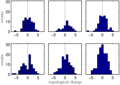
Figure 6: Histograms of the topological charge for the E data set, split up by independent series.

V The chiral condensate and matching masses

With the $M=m\Sigma V$ values predicted from the topological charge distribution we are now able to extract the physical value of the chiral condensate. Combining the $M$ values with $r_{0}/a$ from Table 1 we find that all four configuration sets predict a consistent value for the $\Sigma$ condensate, as listed in Table 2. The only sign that the light L set differs from the RMT prediction more than the other mass values is the larger error of the predicted condensate. The value we obtain,

$$\Sigma_{\mathrm{lat}}^{1/3}=291(5)\,\mathrm{MeV}$$ (7)

is the lattice condensate. To connect it to a more conventional scheme, like $\overline{\mathrm{MS}}$ at 2 GeV, one needs the corresponding renormalization factor $Z_{s}$. Such a factor should be calculated non-perturbatively on the staggered configurations with our specific valence Dirac operator. We have not done this calculation yet but similar ones exist. The same Dirac operator was used on a quenched data set in DeGrand and Liu (2005), while a similar one with stout instead of HYP smearing on $n_{f}=1$ and 2 dynamical configurations was used in DeGrand et al. (2006a, b). $Z_{s}$ seems to be largely independent of the detailed properties of the background configurations and we estimate its value to be

$$Z_{s}\geq 0.9\;,$$ (8)

which could lower the value of $\Sigma^{1/3}$ by 3%. In addition, there is a finite volume correction that could be rather large, up to 10-15% for $\Sigma^{1/3}$ Damgaard (2002); DeGrand (2006), further decreasing the value of the condensate. These effects will have to be investigated but they are beyond the scope of the present paper.

The value of the condensate in Eq.(7) is consistent with predictions obtained on overlap dynamical configurations DeGrand et al. (2006b). The agreement further supports our observation that the rooted staggered configurations are QCD like, the non-local terms of the action can be simply taken into account as lattice artifacts. Of course to really support this statement one has to repeat the calculation at different lattice spacings. Such a study is under way and its result will be reported separately.

Finally we turn our attention to the matching overlap mass values. Combining $M$ and $\Sigma$ we get the values listed in the ”$am$” column of Table 2. These matching masses are not only surprisingly large but they do not depend linearly on the staggered masses. While the staggered quark mass changes a factor of four between the lightest and heaviest data sets, the matching overlap masses change only 50% . This is similar to what we observed in the Schwinger model Hasenfratz and Hoffmann (2006a), the matching valence masses show an overall shift compared to the staggered sea mass values. In addition at very small sea quark masses, where the matching breaks down, the valence quark masses are largely independent of the sea quark mass values. This is illustrated in Fig. 3 of Ref. Hasenfratz and Hoffmann (2006a). Such behavior implies that staggered configurations at small quark masses are not necessarily closer to chiral continuum QCD than the heavier mass configurations. All the computational efforts creating light configurations could be in vain, creating only configurations with larger lattice artifacts. This might not be a problem when the data is analyzed with the whole machinery of staggered partially quenched chiral perturbation theory but should be considered when individual configuration sets are analyzed in mixed action simulations. Of course this is only a lattice artifact and any such effect will disappear as the continuum limit is approached.

As a final comment we note that staggered chiral perturbation theory indicates that at leading order the topological susceptibility depends on the taste singlet pion Billeter et al. (2004). That is the heaviest of the pseudoscalars and it is quite conceivable that our matching procedure identified a quark mass corresponding to this pion. To test that assertion one would have to measure the overlap pion spectrum on the staggered background configurations.

VI Conclusion

We have studied the properties of the rooted staggered action in a mixed action simulation using overlap valence quarks. By comparing physical quantities that are independent of the valence quark mass to continuum QCD predictions we can identify lattice artifacts and study their dependence on the lattice spacing and sea quark masses. In this work we considered the eigenvalue distribution of the massless Dirac operator and the distribution of the topological charge. We compared the former to the universal predictions of random matrix theory and found that the systematic deviation of the data from the predictions were comparable to quenched and dynamical overlap simulations, especially at larger sea quark masses. Using the topological charge distribution we could identify the matching overlap valence quark mass value which best describes the staggered configurations. We found these matching values to be fairly large and their dependence on the staggered sea mass values is not consistent with a simple linear renormalization factor. With the use of the matching mass we extracted the value of the chiral scalar condensate. We found that the predictions from all of our staggered configuration sets were consistent. These findings indicate that at our lattice spacing, $a\!\approx\!0.13\,$fm, and with not very light sea quarks the rooted staggered lattice configurations have lattice artifacts similar to other lattice action, the non-local terms arising from the rooting procedure can be simply considered as part of the cutoff effects. In order to show that these non-local terms indeed become irrelevant in the continuum limit the calculation have to be repeated at different lattice spacings and the scaling of the lattice artifacts investigated. It would also be important to study in a similar manner the lattice artifacts of other observables.