PHENIX Collaboration

Identified Charged Particle Spectra and Yields
in Au+Au Collisions at $\sqrt{s_{NN}}$ = 200 GeV

S.S. Adler Brookhaven National Laboratory, Upton, NY 11973-5000, USA S. Afanasiev Joint Institute for Nuclear Research, 141980 Dubna, Moscow Region, Russia C. Aidala Brookhaven National Laboratory, Upton, NY 11973-5000, USA N.N. Ajitanand Chemistry Department, Stony Brook University, SUNY, Stony Brook, NY 11794-3400, USA Y. Akiba KEK, High Energy Accelerator Research Organization, Tsukuba-shi, Ibaraki-ken 305-0801, Japan RIKEN (The Institute of Physical and Chemical Research), Wako, Saitama 351-0198, JAPAN J. Alexander Chemistry Department, Stony Brook University, SUNY, Stony Brook, NY 11794-3400, USA R. Amirikas Florida State University, Tallahassee, FL 32306, USA L. Aphecetche SUBATECH (Ecole des Mines de Nantes, CNRS-IN2P3, Université de Nantes) BP 20722 - 44307, Nantes, France S.H. Aronson Brookhaven National Laboratory, Upton, NY 11973-5000, USA R. Averbeck Department of Physics and Astronomy, Stony Brook University, SUNY, Stony Brook, NY 11794, USA T.C. Awes Oak Ridge National Laboratory, Oak Ridge, TN 37831, USA R. Azmoun Department of Physics and Astronomy, Stony Brook University, SUNY, Stony Brook, NY 11794, USA V. Babintsev Institute for High Energy Physics (IHEP), Protvino, Russia A. Baldisseri Dapnia, CEA Saclay, F-91191, Gif-sur-Yvette, France K.N. Barish University of California - Riverside, Riverside, CA 92521, USA P.D. Barnes Los Alamos National Laboratory, Los Alamos, NM 87545, USA B. Bassalleck University of New Mexico, Albuquerque, NM, USA S. Bathe Institut fuer Kernphysik, University of Muenster, D-48149 Muenster, Germany S. Batsouli Columbia University, New York, NY 10027 and Nevis Laboratories, Irvington, NY 10533, USA V. Baublis PNPI, Petersburg Nuclear Physics Institute, Gatchina, Russia A. Bazilevsky RIKEN BNL Research Center, Brookhaven National Laboratory, Upton, NY 11973-5000, USA Institute for High Energy Physics (IHEP), Protvino, Russia S. Belikov Iowa State University, Ames, IA 50011, USA Institute for High Energy Physics (IHEP), Protvino, Russia Y. Berdnikov St. Petersburg State Technical University, St. Petersburg, Russia S. Bhagavatula Iowa State University, Ames, IA 50011, USA J.G. Boissevain Los Alamos National Laboratory, Los Alamos, NM 87545, USA H. Borel Dapnia, CEA Saclay, F-91191, Gif-sur-Yvette, France S. Borenstein Laboratoire Leprince-Ringuet, Ecole Polytechnique, CNRS-IN2P3, Route de Saclay, F-91128, Palaiseau, France M.L. Brooks Los Alamos National Laboratory, Los Alamos, NM 87545, USA D.S. Brown New Mexico State University, Las Cruces, NM 88003, USA N. Bruner University of New Mexico, Albuquerque, NM, USA D. Bucher Institut fuer Kernphysik, University of Muenster, D-48149 Muenster, Germany H. Buesching Institut fuer Kernphysik, University of Muenster, D-48149 Muenster, Germany V. Bumazhnov Institute for High Energy Physics (IHEP), Protvino, Russia G. Bunce Brookhaven National Laboratory, Upton, NY 11973-5000, USA RIKEN BNL Research Center, Brookhaven National Laboratory, Upton, NY 11973-5000, USA J.M. Burward-Hoy Lawrence Livermore National Laboratory, Livermore, CA 94550, USA Department of Physics and Astronomy, Stony Brook University, SUNY, Stony Brook, NY 11794, USA S. Butsyk Department of Physics and Astronomy, Stony Brook University, SUNY, Stony Brook, NY 11794, USA X. Camard SUBATECH (Ecole des Mines de Nantes, CNRS-IN2P3, Université de Nantes) BP 20722 - 44307, Nantes, France J.-S. Chai KAERI, Cyclotron Application Laboratory, Seoul, South Korea P. Chand Bhabha Atomic Research Centre, Bombay 400 085, India W.C. Chang Institute of Physics, Academia Sinica, Taipei 11529, Taiwan S. Chernichenko Institute for High Energy Physics (IHEP), Protvino, Russia C.Y. Chi Columbia University, New York, NY 10027 and Nevis Laboratories, Irvington, NY 10533, USA J. Chiba KEK, High Energy Accelerator Research Organization, Tsukuba-shi, Ibaraki-ken 305-0801, Japan M. Chiu Columbia University, New York, NY 10027 and Nevis Laboratories, Irvington, NY 10533, USA I.J. Choi Yonsei University, IPAP, Seoul 120-749, Korea J. Choi Kangnung National University, Kangnung 210-702, South Korea R.K. Choudhury Bhabha Atomic Research Centre, Bombay 400 085, India T. Chujo Brookhaven National Laboratory, Upton, NY 11973-5000, USA V. Cianciolo Oak Ridge National Laboratory, Oak Ridge, TN 37831, USA Y. Cobigo Dapnia, CEA Saclay, F-91191, Gif-sur-Yvette, France B.A. Cole Columbia University, New York, NY 10027 and Nevis Laboratories, Irvington, NY 10533, USA P. Constantin Iowa State University, Ames, IA 50011, USA D.G. d’Enterria SUBATECH (Ecole des Mines de Nantes, CNRS-IN2P3, Université de Nantes) BP 20722 - 44307, Nantes, France G. David Brookhaven National Laboratory, Upton, NY 11973-5000, USA H. Delagrange SUBATECH (Ecole des Mines de Nantes, CNRS-IN2P3, Université de Nantes) BP 20722 - 44307, Nantes, France A. Denisov Institute for High Energy Physics (IHEP), Protvino, Russia A. Deshpande RIKEN BNL Research Center, Brookhaven National Laboratory, Upton, NY 11973-5000, USA E.J. Desmond Brookhaven National Laboratory, Upton, NY 11973-5000, USA O. Dietzsch Universidade de São Paulo, Instituto de Física, Caixa Postal 66318, São Paulo CEP05315-970, Brazil O. Drapier Laboratoire Leprince-Ringuet, Ecole Polytechnique, CNRS-IN2P3, Route de Saclay, F-91128, Palaiseau, France A. Drees Department of Physics and Astronomy, Stony Brook University, SUNY, Stony Brook, NY 11794, USA R. du Rietz Department of Physics, Lund University, Box 118, SE-221 00 Lund, Sweden A. Durum Institute for High Energy Physics (IHEP), Protvino, Russia D. Dutta Bhabha Atomic Research Centre, Bombay 400 085, India Y.V. Efremenko Oak Ridge National Laboratory, Oak Ridge, TN 37831, USA K. El Chenawi Vanderbilt University, Nashville, TN 37235, USA A. Enokizono Hiroshima University, Kagamiyama, Higashi-Hiroshima 739-8526, Japan H. En’yo RIKEN (The Institute of Physical and Chemical Research), Wako, Saitama 351-0198, JAPAN RIKEN BNL Research Center, Brookhaven National Laboratory, Upton, NY 11973-5000, USA S. Esumi Institute of Physics, University of Tsukuba, Tsukuba, Ibaraki 305, Japan L. Ewell Brookhaven National Laboratory, Upton, NY 11973-5000, USA D.E. Fields University of New Mexico, Albuquerque, NM, USA RIKEN BNL Research Center, Brookhaven National Laboratory, Upton, NY 11973-5000, USA F. Fleuret Laboratoire Leprince-Ringuet, Ecole Polytechnique, CNRS-IN2P3, Route de Saclay, F-91128, Palaiseau, France S.L. Fokin Russian Research Center “Kurchatov Institute”, Moscow, Russia B.D. Fox RIKEN BNL Research Center, Brookhaven National Laboratory, Upton, NY 11973-5000, USA Z. Fraenkel Weizmann Institute, Rehovot 76100, Israel J.E. Frantz Columbia University, New York, NY 10027 and Nevis Laboratories, Irvington, NY 10533, USA A. Franz Brookhaven National Laboratory, Upton, NY 11973-5000, USA A.D. Frawley Florida State University, Tallahassee, FL 32306, USA S.-Y. Fung University of California - Riverside, Riverside, CA 92521, USA S. Garpman Deceased Department of Physics, Lund University, Box 118, SE-221 00 Lund, Sweden T.K. Ghosh Vanderbilt University, Nashville, TN 37235, USA A. Glenn University of Tennessee, Knoxville, TN 37996, USA G. Gogiberidze University of Tennessee, Knoxville, TN 37996, USA M. Gonin Laboratoire Leprince-Ringuet, Ecole Polytechnique, CNRS-IN2P3, Route de Saclay, F-91128, Palaiseau, France J. Gosset Dapnia, CEA Saclay, F-91191, Gif-sur-Yvette, France Y. Goto RIKEN BNL Research Center, Brookhaven National Laboratory, Upton, NY 11973-5000, USA R. Granier de Cassagnac Laboratoire Leprince-Ringuet, Ecole Polytechnique, CNRS-IN2P3, Route de Saclay, F-91128, Palaiseau, France N. Grau Iowa State University, Ames, IA 50011, USA S.V. Greene Vanderbilt University, Nashville, TN 37235, USA M. Grosse Perdekamp RIKEN BNL Research Center, Brookhaven National Laboratory, Upton, NY 11973-5000, USA W. Guryn Brookhaven National Laboratory, Upton, NY 11973-5000, USA H.-Å. Gustafsson Department of Physics, Lund University, Box 118, SE-221 00 Lund, Sweden T. Hachiya Hiroshima University, Kagamiyama, Higashi-Hiroshima 739-8526, Japan J.S. Haggerty Brookhaven National Laboratory, Upton, NY 11973-5000, USA H. Hamagaki Center for Nuclear Study, Graduate School of Science, University of Tokyo, 7-3-1 Hongo, Bunkyo, Tokyo 113-0033, Japan A.G. Hansen Los Alamos National Laboratory, Los Alamos, NM 87545, USA E.P. Hartouni Lawrence Livermore National Laboratory, Livermore, CA 94550, USA M. Harvey Brookhaven National Laboratory, Upton, NY 11973-5000, USA R. Hayano Center for Nuclear Study, Graduate School of Science, University of Tokyo, 7-3-1 Hongo, Bunkyo, Tokyo 113-0033, Japan X. He Georgia State University, Atlanta, GA 30303, USA M. Heffner Lawrence Livermore National Laboratory, Livermore, CA 94550, USA T.K. Hemmick Department of Physics and Astronomy, Stony Brook University, SUNY, Stony Brook, NY 11794, USA J.M. Heuser Department of Physics and Astronomy, Stony Brook University, SUNY, Stony Brook, NY 11794, USA M. Hibino Waseda University, Advanced Research Institute for Science and Engineering, 17 Kikui-cho, Shinjuku-ku, Tokyo 162-0044, Japan J.C. Hill Iowa State University, Ames, IA 50011, USA W. Holzmann Chemistry Department, Stony Brook University, SUNY, Stony Brook, NY 11794-3400, USA K. Homma Hiroshima University, Kagamiyama, Higashi-Hiroshima 739-8526, Japan B. Hong Korea University, Seoul, 136-701, Korea A. Hoover New Mexico State University, Las Cruces, NM 88003, USA T. Ichihara RIKEN (The Institute of Physical and Chemical Research), Wako, Saitama 351-0198, JAPAN RIKEN BNL Research Center, Brookhaven National Laboratory, Upton, NY 11973-5000, USA V.V. Ikonnikov Russian Research Center “Kurchatov Institute”, Moscow, Russia K. Imai Kyoto University, Kyoto 606, Japan RIKEN (The Institute of Physical and Chemical Research), Wako, Saitama 351-0198, JAPAN D. Isenhower Abilene Christian University, Abilene, TX 79699, USA M. Ishihara RIKEN (The Institute of Physical and Chemical Research), Wako, Saitama 351-0198, JAPAN M. Issah Chemistry Department, Stony Brook University, SUNY, Stony Brook, NY 11794-3400, USA A. Isupov Joint Institute for Nuclear Research, 141980 Dubna, Moscow Region, Russia B.V. Jacak Department of Physics and Astronomy, Stony Brook University, SUNY, Stony Brook, NY 11794, USA W.Y. Jang Korea University, Seoul, 136-701, Korea Y. Jeong Kangnung National University, Kangnung 210-702, South Korea J. Jia Department of Physics and Astronomy, Stony Brook University, SUNY, Stony Brook, NY 11794, USA O. Jinnouchi RIKEN (The Institute of Physical and Chemical Research), Wako, Saitama 351-0198, JAPAN B.M. Johnson Brookhaven National Laboratory, Upton, NY 11973-5000, USA S.C. Johnson Lawrence Livermore National Laboratory, Livermore, CA 94550, USA K.S. Joo Myongji University, Yongin, Kyonggido 449-728, Korea D. Jouan IPN-Orsay, Universite Paris Sud, CNRS-IN2P3, BP1, F-91406, Orsay, France S. Kametani Center for Nuclear Study, Graduate School of Science, University of Tokyo, 7-3-1 Hongo, Bunkyo, Tokyo 113-0033, Japan Waseda University, Advanced Research Institute for Science and Engineering, 17 Kikui-cho, Shinjuku-ku, Tokyo 162-0044, Japan N. Kamihara Department of Physics, Tokyo Institute of Technology, Tokyo, 152-8551, Japan RIKEN (The Institute of Physical and Chemical Research), Wako, Saitama 351-0198, JAPAN J.H. Kang Yonsei University, IPAP, Seoul 120-749, Korea S.S. Kapoor Bhabha Atomic Research Centre, Bombay 400 085, India K. Katou Waseda University, Advanced Research Institute for Science and Engineering, 17 Kikui-cho, Shinjuku-ku, Tokyo 162-0044, Japan S. Kelly Columbia University, New York, NY 10027 and Nevis Laboratories, Irvington, NY 10533, USA B. Khachaturov Weizmann Institute, Rehovot 76100, Israel A. Khanzadeev PNPI, Petersburg Nuclear Physics Institute, Gatchina, Russia J. Kikuchi Waseda University, Advanced Research Institute for Science and Engineering, 17 Kikui-cho, Shinjuku-ku, Tokyo 162-0044, Japan D.H. Kim Myongji University, Yongin, Kyonggido 449-728, Korea D.J. Kim Yonsei University, IPAP, Seoul 120-749, Korea D.W. Kim Kangnung National University, Kangnung 210-702, South Korea E. Kim System Electronics Laboratory, Seoul National University, Seoul, South Korea G.-B. Kim Laboratoire Leprince-Ringuet, Ecole Polytechnique, CNRS-IN2P3, Route de Saclay, F-91128, Palaiseau, France H.J. Kim Yonsei University, IPAP, Seoul 120-749, Korea E. Kistenev Brookhaven National Laboratory, Upton, NY 11973-5000, USA A. Kiyomichi Institute of Physics, University of Tsukuba, Tsukuba, Ibaraki 305, Japan K. Kiyoyama Nagasaki Institute of Applied Science, Nagasaki-shi, Nagasaki 851-0193, Japan C. Klein-Boesing Institut fuer Kernphysik, University of Muenster, D-48149 Muenster, Germany H. Kobayashi RIKEN (The Institute of Physical and Chemical Research), Wako, Saitama 351-0198, JAPAN RIKEN BNL Research Center, Brookhaven National Laboratory, Upton, NY 11973-5000, USA L. Kochenda PNPI, Petersburg Nuclear Physics Institute, Gatchina, Russia V. Kochetkov Institute for High Energy Physics (IHEP), Protvino, Russia D. Koehler University of New Mexico, Albuquerque, NM, USA T. Kohama Hiroshima University, Kagamiyama, Higashi-Hiroshima 739-8526, Japan M. Kopytine Department of Physics and Astronomy, Stony Brook University, SUNY, Stony Brook, NY 11794, USA D. Kotchetkov University of California - Riverside, Riverside, CA 92521, USA A. Kozlov Weizmann Institute, Rehovot 76100, Israel P.J. Kroon Brookhaven National Laboratory, Upton, NY 11973-5000, USA C.H. Kuberg Abilene Christian University, Abilene, TX 79699, USA Los Alamos National Laboratory, Los Alamos, NM 87545, USA K. Kurita RIKEN BNL Research Center, Brookhaven National Laboratory, Upton, NY 11973-5000, USA Y. Kuroki Institute of Physics, University of Tsukuba, Tsukuba, Ibaraki 305, Japan M.J. Kweon Korea University, Seoul, 136-701, Korea Y. Kwon Yonsei University, IPAP, Seoul 120-749, Korea G.S. Kyle New Mexico State University, Las Cruces, NM 88003, USA R. Lacey Chemistry Department, Stony Brook University, SUNY, Stony Brook, NY 11794-3400, USA V. Ladygin Joint Institute for Nuclear Research, 141980 Dubna, Moscow Region, Russia J.G. Lajoie Iowa State University, Ames, IA 50011, USA A. Lebedev Iowa State University, Ames, IA 50011, USA Russian Research Center “Kurchatov Institute”, Moscow, Russia S. Leckey Department of Physics and Astronomy, Stony Brook University, SUNY, Stony Brook, NY 11794, USA D.M. Lee Los Alamos National Laboratory, Los Alamos, NM 87545, USA S. Lee Kangnung National University, Kangnung 210-702, South Korea M.J. Leitch Los Alamos National Laboratory, Los Alamos, NM 87545, USA X.H. Li University of California - Riverside, Riverside, CA 92521, USA H. Lim System Electronics Laboratory, Seoul National University, Seoul, South Korea A. Litvinenko Joint Institute for Nuclear Research, 141980 Dubna, Moscow Region, Russia M.X. Liu Los Alamos National Laboratory, Los Alamos, NM 87545, USA Y. Liu IPN-Orsay, Universite Paris Sud, CNRS-IN2P3, BP1, F-91406, Orsay, France C.F. Maguire Vanderbilt University, Nashville, TN 37235, USA Y.I. Makdisi Brookhaven National Laboratory, Upton, NY 11973-5000, USA A. Malakhov Joint Institute for Nuclear Research, 141980 Dubna, Moscow Region, Russia V.I. Manko Russian Research Center “Kurchatov Institute”, Moscow, Russia Y. Mao China Institute of Atomic Energy (CIAE), Beijing, People’s Republic of China RIKEN (The Institute of Physical and Chemical Research), Wako, Saitama 351-0198, JAPAN G. Martinez SUBATECH (Ecole des Mines de Nantes, CNRS-IN2P3, Université de Nantes) BP 20722 - 44307, Nantes, France M.D. Marx Department of Physics and Astronomy, Stony Brook University, SUNY, Stony Brook, NY 11794, USA H. Masui Institute of Physics, University of Tsukuba, Tsukuba, Ibaraki 305, Japan F. Matathias Department of Physics and Astronomy, Stony Brook University, SUNY, Stony Brook, NY 11794, USA T. Matsumoto Center for Nuclear Study, Graduate School of Science, University of Tokyo, 7-3-1 Hongo, Bunkyo, Tokyo 113-0033, Japan Waseda University, Advanced Research Institute for Science and Engineering, 17 Kikui-cho, Shinjuku-ku, Tokyo 162-0044, Japan P.L. McGaughey Los Alamos National Laboratory, Los Alamos, NM 87545, USA E. Melnikov Institute for High Energy Physics (IHEP), Protvino, Russia F. Messer Department of Physics and Astronomy, Stony Brook University, SUNY, Stony Brook, NY 11794, USA Y. Miake Institute of Physics, University of Tsukuba, Tsukuba, Ibaraki 305, Japan J. Milan Chemistry Department, Stony Brook University, SUNY, Stony Brook, NY 11794-3400, USA T.E. Miller Vanderbilt University, Nashville, TN 37235, USA A. Milov Department of Physics and Astronomy, Stony Brook University, SUNY, Stony Brook, NY 11794, USA Weizmann Institute, Rehovot 76100, Israel S. Mioduszewski Brookhaven National Laboratory, Upton, NY 11973-5000, USA R.E. Mischke Los Alamos National Laboratory, Los Alamos, NM 87545, USA G.C. Mishra Georgia State University, Atlanta, GA 30303, USA J.T. Mitchell Brookhaven National Laboratory, Upton, NY 11973-5000, USA A.K. Mohanty Bhabha Atomic Research Centre, Bombay 400 085, India D.P. Morrison Brookhaven National Laboratory, Upton, NY 11973-5000, USA J.M. Moss Los Alamos National Laboratory, Los Alamos, NM 87545, USA F. Mühlbacher Department of Physics and Astronomy, Stony Brook University, SUNY, Stony Brook, NY 11794, USA D. Mukhopadhyay Weizmann Institute, Rehovot 76100, Israel M. Muniruzzaman University of California - Riverside, Riverside, CA 92521, USA J. Murata RIKEN (The Institute of Physical and Chemical Research), Wako, Saitama 351-0198, JAPAN RIKEN BNL Research Center, Brookhaven National Laboratory, Upton, NY 11973-5000, USA S. Nagamiya KEK, High Energy Accelerator Research Organization, Tsukuba-shi, Ibaraki-ken 305-0801, Japan J.L. Nagle Columbia University, New York, NY 10027 and Nevis Laboratories, Irvington, NY 10533, USA T. Nakamura Hiroshima University, Kagamiyama, Higashi-Hiroshima 739-8526, Japan B.K. Nandi University of California - Riverside, Riverside, CA 92521, USA M. Nara Institute of Physics, University of Tsukuba, Tsukuba, Ibaraki 305, Japan J. Newby University of Tennessee, Knoxville, TN 37996, USA P. Nilsson Department of Physics, Lund University, Box 118, SE-221 00 Lund, Sweden A.S. Nyanin Russian Research Center “Kurchatov Institute”, Moscow, Russia J. Nystrand Department of Physics, Lund University, Box 118, SE-221 00 Lund, Sweden E. O’Brien Brookhaven National Laboratory, Upton, NY 11973-5000, USA C.A. Ogilvie Iowa State University, Ames, IA 50011, USA H. Ohnishi Brookhaven National Laboratory, Upton, NY 11973-5000, USA RIKEN (The Institute of Physical and Chemical Research), Wako, Saitama 351-0198, JAPAN I.D. Ojha Vanderbilt University, Nashville, TN 37235, USA Department of Physics, Banaras Hindu University, Varanasi 221005, India K. Okada RIKEN (The Institute of Physical and Chemical Research), Wako, Saitama 351-0198, JAPAN M. Ono Institute of Physics, University of Tsukuba, Tsukuba, Ibaraki 305, Japan V. Onuchin Institute for High Energy Physics (IHEP), Protvino, Russia A. Oskarsson Department of Physics, Lund University, Box 118, SE-221 00 Lund, Sweden I. Otterlund Department of Physics, Lund University, Box 118, SE-221 00 Lund, Sweden K. Oyama Center for Nuclear Study, Graduate School of Science, University of Tokyo, 7-3-1 Hongo, Bunkyo, Tokyo 113-0033, Japan K. Ozawa Center for Nuclear Study, Graduate School of Science, University of Tokyo, 7-3-1 Hongo, Bunkyo, Tokyo 113-0033, Japan D. Pal Weizmann Institute, Rehovot 76100, Israel A.P.T. Palounek Los Alamos National Laboratory, Los Alamos, NM 87545, USA V.S. Pantuev Department of Physics and Astronomy, Stony Brook University, SUNY, Stony Brook, NY 11794, USA V. Papavassiliou New Mexico State University, Las Cruces, NM 88003, USA J. Park System Electronics Laboratory, Seoul National University, Seoul, South Korea A. Parmar University of New Mexico, Albuquerque, NM, USA S.F. Pate New Mexico State University, Las Cruces, NM 88003, USA T. Peitzmann Institut fuer Kernphysik, University of Muenster, D-48149 Muenster, Germany J.-C. Peng Los Alamos National Laboratory, Los Alamos, NM 87545, USA V. Peresedov Joint Institute for Nuclear Research, 141980 Dubna, Moscow Region, Russia C. Pinkenburg Brookhaven National Laboratory, Upton, NY 11973-5000, USA R.P. Pisani Brookhaven National Laboratory, Upton, NY 11973-5000, USA F. Plasil Oak Ridge National Laboratory, Oak Ridge, TN 37831, USA M.L. Purschke Brookhaven National Laboratory, Upton, NY 11973-5000, USA A.K. Purwar Department of Physics and Astronomy, Stony Brook University, SUNY, Stony Brook, NY 11794, USA J. Rak Iowa State University, Ames, IA 50011, USA I. Ravinovich Weizmann Institute, Rehovot 76100, Israel K.F. Read Oak Ridge National Laboratory, Oak Ridge, TN 37831, USA University of Tennessee, Knoxville, TN 37996, USA M. Reuter Department of Physics and Astronomy, Stony Brook University, SUNY, Stony Brook, NY 11794, USA K. Reygers Institut fuer Kernphysik, University of Muenster, D-48149 Muenster, Germany V. Riabov PNPI, Petersburg Nuclear Physics Institute, Gatchina, Russia St. Petersburg State Technical University, St. Petersburg, Russia Y. Riabov PNPI, Petersburg Nuclear Physics Institute, Gatchina, Russia G. Roche LPC, Université Blaise Pascal, CNRS-IN2P3, Clermont-Fd, 63177 Aubiere Cedex, France A. Romana Laboratoire Leprince-Ringuet, Ecole Polytechnique, CNRS-IN2P3, Route de Saclay, F-91128, Palaiseau, France M. Rosati Iowa State University, Ames, IA 50011, USA P. Rosnet LPC, Université Blaise Pascal, CNRS-IN2P3, Clermont-Fd, 63177 Aubiere Cedex, France S.S. Ryu Yonsei University, IPAP, Seoul 120-749, Korea M.E. Sadler Abilene Christian University, Abilene, TX 79699, USA N. Saito RIKEN (The Institute of Physical and Chemical Research), Wako, Saitama 351-0198, JAPAN RIKEN BNL Research Center, Brookhaven National Laboratory, Upton, NY 11973-5000, USA T. Sakaguchi Center for Nuclear Study, Graduate School of Science, University of Tokyo, 7-3-1 Hongo, Bunkyo, Tokyo 113-0033, Japan Waseda University, Advanced Research Institute for Science and Engineering, 17 Kikui-cho, Shinjuku-ku, Tokyo 162-0044, Japan M. Sakai Nagasaki Institute of Applied Science, Nagasaki-shi, Nagasaki 851-0193, Japan S. Sakai Institute of Physics, University of Tsukuba, Tsukuba, Ibaraki 305, Japan V. Samsonov PNPI, Petersburg Nuclear Physics Institute, Gatchina, Russia L. Sanfratello University of New Mexico, Albuquerque, NM, USA R. Santo Institut fuer Kernphysik, University of Muenster, D-48149 Muenster, Germany H.D. Sato Kyoto University, Kyoto 606, Japan RIKEN (The Institute of Physical and Chemical Research), Wako, Saitama 351-0198, JAPAN S. Sato Brookhaven National Laboratory, Upton, NY 11973-5000, USA Institute of Physics, University of Tsukuba, Tsukuba, Ibaraki 305, Japan S. Sawada KEK, High Energy Accelerator Research Organization, Tsukuba-shi, Ibaraki-ken 305-0801, Japan Y. Schutz SUBATECH (Ecole des Mines de Nantes, CNRS-IN2P3, Université de Nantes) BP 20722 - 44307, Nantes, France V. Semenov Institute for High Energy Physics (IHEP), Protvino, Russia R. Seto University of California - Riverside, Riverside, CA 92521, USA M.R. Shaw Abilene Christian University, Abilene, TX 79699, USA Los Alamos National Laboratory, Los Alamos, NM 87545, USA T.K. Shea Brookhaven National Laboratory, Upton, NY 11973-5000, USA T.-A. Shibata Department of Physics, Tokyo Institute of Technology, Tokyo, 152-8551, Japan RIKEN (The Institute of Physical and Chemical Research), Wako, Saitama 351-0198, JAPAN K. Shigaki Hiroshima University, Kagamiyama, Higashi-Hiroshima 739-8526, Japan KEK, High Energy Accelerator Research Organization, Tsukuba-shi, Ibaraki-ken 305-0801, Japan T. Shiina Los Alamos National Laboratory, Los Alamos, NM 87545, USA C.L. Silva Universidade de São Paulo, Instituto de Física, Caixa Postal 66318, São Paulo CEP05315-970, Brazil D. Silvermyr Los Alamos National Laboratory, Los Alamos, NM 87545, USA Department of Physics, Lund University, Box 118, SE-221 00 Lund, Sweden K.S. Sim Korea University, Seoul, 136-701, Korea C.P. Singh Department of Physics, Banaras Hindu University, Varanasi 221005, India V. Singh Department of Physics, Banaras Hindu University, Varanasi 221005, India M. Sivertz Brookhaven National Laboratory, Upton, NY 11973-5000, USA A. Soldatov Institute for High Energy Physics (IHEP), Protvino, Russia R.A. Soltz Lawrence Livermore National Laboratory, Livermore, CA 94550, USA W.E. Sondheim Los Alamos National Laboratory, Los Alamos, NM 87545, USA S.P. Sorensen University of Tennessee, Knoxville, TN 37996, USA I.V. Sourikova Brookhaven National Laboratory, Upton, NY 11973-5000, USA F. Staley Dapnia, CEA Saclay, F-91191, Gif-sur-Yvette, France P.W. Stankus Oak Ridge National Laboratory, Oak Ridge, TN 37831, USA E. Stenlund Department of Physics, Lund University, Box 118, SE-221 00 Lund, Sweden M. Stepanov New Mexico State University, Las Cruces, NM 88003, USA A. Ster KFKI Research Institute for Particle and Nuclear Physics (RMKI), H-1525 Budapest 114, POBox 49, Hungary S.P. Stoll Brookhaven National Laboratory, Upton, NY 11973-5000, USA T. Sugitate Hiroshima University, Kagamiyama, Higashi-Hiroshima 739-8526, Japan J.P. Sullivan Los Alamos National Laboratory, Los Alamos, NM 87545, USA E.M. Takagui Universidade de São Paulo, Instituto de Física, Caixa Postal 66318, São Paulo CEP05315-970, Brazil A. Taketani RIKEN (The Institute of Physical and Chemical Research), Wako, Saitama 351-0198, JAPAN RIKEN BNL Research Center, Brookhaven National Laboratory, Upton, NY 11973-5000, USA M. Tamai Waseda University, Advanced Research Institute for Science and Engineering, 17 Kikui-cho, Shinjuku-ku, Tokyo 162-0044, Japan K.H. Tanaka KEK, High Energy Accelerator Research Organization, Tsukuba-shi, Ibaraki-ken 305-0801, Japan Y. Tanaka Nagasaki Institute of Applied Science, Nagasaki-shi, Nagasaki 851-0193, Japan K. Tanida RIKEN (The Institute of Physical and Chemical Research), Wako, Saitama 351-0198, JAPAN M.J. Tannenbaum Brookhaven National Laboratory, Upton, NY 11973-5000, USA P. Tarján Debrecen University, H-4010 Debrecen, Egyetem tér 1, Hungary J.D. Tepe Abilene Christian University, Abilene, TX 79699, USA Los Alamos National Laboratory, Los Alamos, NM 87545, USA T.L. Thomas University of New Mexico, Albuquerque, NM, USA J. Tojo Kyoto University, Kyoto 606, Japan RIKEN (The Institute of Physical and Chemical Research), Wako, Saitama 351-0198, JAPAN H. Torii Kyoto University, Kyoto 606, Japan RIKEN (The Institute of Physical and Chemical Research), Wako, Saitama 351-0198, JAPAN R.S. Towell Abilene Christian University, Abilene, TX 79699, USA I. Tserruya Weizmann Institute, Rehovot 76100, Israel H. Tsuruoka Institute of Physics, University of Tsukuba, Tsukuba, Ibaraki 305, Japan S.K. Tuli Department of Physics, Banaras Hindu University, Varanasi 221005, India H. Tydesjö Department of Physics, Lund University, Box 118, SE-221 00 Lund, Sweden N. Tyurin Institute for High Energy Physics (IHEP), Protvino, Russia H.W. van Hecke Los Alamos National Laboratory, Los Alamos, NM 87545, USA J. Velkovska Brookhaven National Laboratory, Upton, NY 11973-5000, USA Department of Physics and Astronomy, Stony Brook University, SUNY, Stony Brook, NY 11794, USA M. Velkovsky Department of Physics and Astronomy, Stony Brook University, SUNY, Stony Brook, NY 11794, USA L. Villatte University of Tennessee, Knoxville, TN 37996, USA A.A. Vinogradov Russian Research Center “Kurchatov Institute”, Moscow, Russia M.A. Volkov Russian Research Center “Kurchatov Institute”, Moscow, Russia E. Vznuzdaev PNPI, Petersburg Nuclear Physics Institute, Gatchina, Russia X.R. Wang Georgia State University, Atlanta, GA 30303, USA Y. Watanabe RIKEN (The Institute of Physical and Chemical Research), Wako, Saitama 351-0198, JAPAN RIKEN BNL Research Center, Brookhaven National Laboratory, Upton, NY 11973-5000, USA S.N. White Brookhaven National Laboratory, Upton, NY 11973-5000, USA F.K. Wohn Iowa State University, Ames, IA 50011, USA C.L. Woody Brookhaven National Laboratory, Upton, NY 11973-5000, USA W. Xie University of California - Riverside, Riverside, CA 92521, USA Y. Yang China Institute of Atomic Energy (CIAE), Beijing, People’s Republic of China A. Yanovich Institute for High Energy Physics (IHEP), Protvino, Russia S. Yokkaichi RIKEN (The Institute of Physical and Chemical Research), Wako, Saitama 351-0198, JAPAN RIKEN BNL Research Center, Brookhaven National Laboratory, Upton, NY 11973-5000, USA G.R. Young Oak Ridge National Laboratory, Oak Ridge, TN 37831, USA I.E. Yushmanov Russian Research Center “Kurchatov Institute”, Moscow, Russia W.A. Zajc zajc@nevis.columbia.edu Columbia University, New York, NY 10027 and Nevis Laboratories, Irvington, NY 10533, USA C. Zhang Columbia University, New York, NY 10027 and Nevis Laboratories, Irvington, NY 10533, USA S. Zhou China Institute of Atomic Energy (CIAE), Beijing, People’s Republic of China Weizmann Institute, Rehovot 76100, Israel L. Zolin Joint Institute for Nuclear Research, 141980 Dubna, Moscow Region, Russia

Abstract

The centrality dependence of transverse momentum distributions and yields for $\pi^{\pm}$ , $K^{\pm}$ , $p$ and $\overline{p}$ in Au+Au collisions at $\sqrt{s_{NN}}$ = 200 GeV at mid-rapidity are measured by the PHENIX experiment at RHIC. We observe a clear particle mass dependence of the shapes of transverse momentum spectra in central collisions below $\sim$ 2 GeV/ $c$ in $p_{T}$ . Both mean transverse momenta and particle yields per participant pair increase from peripheral to mid-central and saturate at the most central collisions for all particle species. We also measure particle ratios of $\pi^{-}/\pi^{+}$ , $K^{-}/K^{+}$ , $\mbox{$\overline{p}$}/p$ , $K/\pi$ , $p/\pi$ and $\mbox{$\overline{p}$}/\pi$ as a function of $p_{T}$ and collision centrality. The ratios of equal mass particle yields are independent of $p_{T}$ and centrality within the experimental uncertainties. In central collisions at intermediate transverse momenta $\sim$ 1.5 – 4.5 GeV/ $c$ , proton and anti-proton yields constitute a significant fraction of the charged hadron production and show a scaling behavior different from that of pions.

pacs:

25.75.Dw

I INTRODUCTION

The motivation for ultra-relativistic heavy-ion experiments at the Relativistic Heavy Ion Collider (RHIC) at Brookhaven National Laboratory is the study of nuclear matter at extremely high temperature and energy density with the hope of creating and detecting deconfined matter consisting of quarks and gluons – the quark gluon plasma (QGP). Lattice QCD calculations lattice predict that the transition to a deconfined state occurs at a critical temperature $T_{c}\approx$ 170 MeV and an energy density $\epsilon\approx$ 2 GeV/ ${\rm fm^{3}}$ . Based on the Bjorken estimation bjorken and the measurement of transverse energy ( $E_{T}$ ) in Au+Au collisions at $\sqrt{s_{NN}}$ = 130 GeV PPG002 and 200 GeV, the spatial energy density in central Au+Au collisions at RHIC is believed to be high enough to create such deconfined matter in a laboratory PPG002 .

The hot and dense matter produced in relativistic heavy ion collisions may evolve through the following scenario: pre-equilibrium, thermal (or chemical) equilibrium of partons, possible formation of QGP or a QGP-hadron gas mixed state, a gas of hot interacting hadrons, and finally, a freeze-out state when the produced hadrons no longer strongly interact with each other. Since produced hadrons carry information about the collision dynamics and the entire space-time evolution of the system from the initial to the final stage of collisions, a precise measure of the transverse momentum ( $p_{T}$ ) distributions and yields of identified hadrons as a function of collision geometry is essential for the understanding of the dynamics and properties of the created matter.

In the low $p_{T}$ region ( $<$ 2 GeV/ $c$ ), hydrodynamic models hydro_1 ; hydro_2 that include radial flow successfully describe the measured $p_{T}$ distributions in Au+Au collisions at $\sqrt{s_{NN}}$ = 130 GeV PPG006 ; STAR_pbar_spectra ; PPG009 . The $p_{T}$ spectra of identified charged hadrons below $\mbox{$p_{T}$}\approx$ 2 GeV/ $c$ in central collisions have been well reproduced by two simple parameters: transverse flow velocity $\beta_{T}$ and freeze-out temperature $T_{fo}$ PPG009 under the assumption of thermalization with longitudinal and transverse flow hydro_1 . The particle production in this $p_{T}$ region is considered to be dominated by secondary interactions among produced hadrons and participating nucleons in the reaction zone. Another model which successfully describes the particle abundances at low $p_{T}$ is the statistical thermal model thermal_becattini . Particle ratios have been shown to be well reproduced by two parameters: a baryon chemical potential $\mu_{B}$ and a chemical freeze-out temperature $T_{ch}$ . It is found that there is an overall good agreement between measured particle ratios at $\sqrt{s_{NN}}$ = 130 GeV Au+Au and the thermal model calculations thermal_1 ; thermal_2 .

On the other hand, at high $p_{T}$ ( $\geq$ 4 GeV/ $c$ ) the dominant particle production mechanism is the hard scattering described by perturbative Quantum Chromodynamics (pQCD), which produces particles from the fragmentation of energetic partons. One of the most interesting observations at RHIC is that the yield of high $p_{T}$ neutral pions and non-identified charged hadrons in central Au+Au collisions at RHIC are below the expectation of the scaling with the number of nucleon-nucleon binary collisions, $N_{coll}$ PPG003 ; PPG013 ; PPG014 . This effect could be a consequence of the energy loss suffered by partons moving through deconfined matter quench_effect ; quenching_theory . It has also been observed that the yield of neutral pions is more strongly suppressed than that for non-identified charged hadrons PPG003 in central Au+Au collisions at RHIC. Another interesting feature is that the proton and anti-proton yields in central events are comparable to that of pions at $\mbox{$p_{T}$}\approx$ 2 GeV/ $c$ PPG006 , differing from the expectation of pQCD. These observations suggest that a detailed study of particle composition at intermediate $p_{T}$ ( $\approx$ 2 – 4 GeV/ $c$ ) is very important to understand hadron production and collision dynamics at RHIC.

The PHENIX experiment PHENIX_overview has a unique hadron identification capability in a broad momentum range. Pions and kaons are identified up to 3 GeV/ $c$ and 2 GeV/ $c$ in $p_{T}$ , respectively, and protons and anti-protons can be identified up to 4.5 GeV/ $c$ by using a high resolution time-of-flight detector PHENIX_PID . Neutral pions are reconstructed via $\mbox{$\pi^{0}$}\rightarrow\gamma\gamma$ up to $\mbox{$p_{T}$}\approx$ 10 GeV/ $c$ through an invariant mass analysis of $\gamma$ pairs detected in an electro-magnetic calorimeter (EMCal) PHENIX_EMC with wide azimuthal coverage. During the measurements of Au+Au collisions at $\sqrt{s_{NN}}$ = 200 GeV in year 2001 at RHIC, the PHENIX experiment accumulated enough events to address the above issues at intermediate $p_{T}$ as well as the particle production at low $p_{T}$ with precise centrality dependences. In this paper, we present the centrality dependence of $p_{T}$ spectra, $\langle p_{T}\rangle$ , yields, and ratios for $\pi^{\pm}$ , $K^{\pm}$ , $p$ and $\overline{p}$ in Au+Au collisions at $\sqrt{s_{NN}}$ = 200 GeV at mid-rapidity measured by the PHENIX experiment. We also present results on the scaling behavior of charged hadrons compared with results of $\pi^{0}$ measurements PPG014 , which have been published separately.

The paper is organized as follows. Section II describes the PHENIX detector used in this analysis. In Section III the analysis details including event selection, track selection, particle identification, and corrections applied to the data are described. The systematic errors on the measurements are also discussed in this section. For the experimental results, centrality dependence of $p_{T}$ spectra for identified charged particles are presented in Section IV.1, and transverse mass spectra are given in Section IV.2. Particle yields and mean transverse momenta as a function of centrality are presented in Section IV.3. In Section IV.4 the systematic study of particle ratios as a function $p_{T}$ and centrality are presented. Section IV.5 studies the scaling behavior of identified charged hadrons. A summary is given in Section V.

II PHENIX DETECTOR

The PHENIX experiment is composed of two central arms, two forward muon arms, and three global detectors. The east and west central arms are placed at zero rapidity and designed to detect electrons, photons and charged hadrons. The north and south forward muon arms have full azimuthal coverage and are designed to detect muons. The global detectors measure the start time, vertex, and multiplicity of the interactions. The following sections describe the parts of the detector that are used in the present analysis. A detailed description of the complete detector can be found elsewhere PHENIX_overview ; PHENIX_PID ; PHENIX_EMC ; PHENIX_inner ; PHENIX_ZDC ; PHENIX_tracking .

II.1 Global Detectors

In order to characterize the centrality of Au+Au collisions, zero-degree calorimeters (ZDC) PHENIX_ZDC and beam-beam counters (BBC) PHENIX_inner are employed. The zero-degree calorimeters are small hadronic calorimeters which measure the energy carried by spectator neutrons. They are placed 18 m up- and downstream of the interaction point along the beam line. Each ZDC consists of three modules. Each module has a depth of 2 hadronic interaction lengths and is read out by a single photo-multiplier tube (PMT). Both time and amplitude are digitized for each PMT along with the analog sum of the three PMT signals for each ZDC.

Two sets of beam-beam counters are placed 1.44 m from the nominal interaction point along the beam line (one on each side). Each counter consists of 64 $\check{\rm C}$ erenkov telescopes, arranged radially around the beam line. The BBC measures the number of charged particles in the pseudo-rapidity region 3.0 $<$ $|\eta|$ $<$ 3.9. The correlation between BBC charge sum and ZDC total energy is used for centrality determination. The BBC also provides a collision vertex position and start time information for time-of-flight measurement.

II.2 Central Arm Detectors

Charged particles are tracked using the central arm spectrometers PHENIX_tracking . The spectrometer on the east side of the PHENIX detector (east arm) contains the following subsystems used in this analysis: drift chamber (DC), pad chamber (PC) and time-of-flight (TOF).

The drift chambers are the closest tracking detectors to the beam line – at a radial distance of 2.2 m. They measure charged particle trajectories in the azimuthal direction to determine the transverse momentum of each particle. By combining the polar angle information from the first layer of the PC with the transverse momentum, the total momentum $p$ is determined. The momentum resolution is $\delta p/p\simeq 0.7\%\oplus 1.0\%\times p$ (GeV/ $c$ ), where the first term is due to the multiple scattering before the DC and the second term is the angular resolution of the DC. The momentum scale is known to 0.7%, from the reconstructed proton mass using the TOF.

The pad chambers are multi-wire proportional chambers that form three separate layers of the central tracking system. The first pad chamber layer (PC1) is located at the radial outer edge of each drift chamber at a distance of 2.49 m, while the third layer (PC3) is 4.98 m from the interaction point. The second layer (PC2) is located at a radial distance of 4.19 m in the west arm only. PC1 and the DC, along with the vertex position measured by the BBC, are used in the global track reconstruction to determine the polar angle of each charged track.

The time-of-flight detector serves as the primary particle identification device for charged hadrons by measuring the stop time. The start time is given by the BBC. The TOF wall is located at a radial distance of 5.06 m from the interaction point in the east central arm. This contains 960 scintillator slats oriented along the azimuthal direction. It is designed to cover $|\eta|<0.35$ and $\Delta\phi=45^{o}$ in azimuthal angle. The intrinsic timing resolution is $\sigma\simeq 115$ ps, which allows for a 3 $\sigma$ $\pi/K$ separation up to $\mbox{$p_{T}$}\simeq 2.5$ GeV/ $c$ , and 3 $\sigma$ $K/p$ separation up to $\mbox{$p_{T}$}\simeq 4$ GeV/ $c$ .

III DATA ANALYSIS

In this section, we describe the event and track selection, charged particle identification and various corrections, including geometrical acceptance, particle decay, multiple scattering and absorption effects, detector occupancy corrections and weak decay contributions from $\Lambda$ and $\overline{\Lambda}$ to proton and anti-proton spectra. The estimations of systematic uncertainties on the measurements are addressed at the end of this section.

III.1 Event Selection

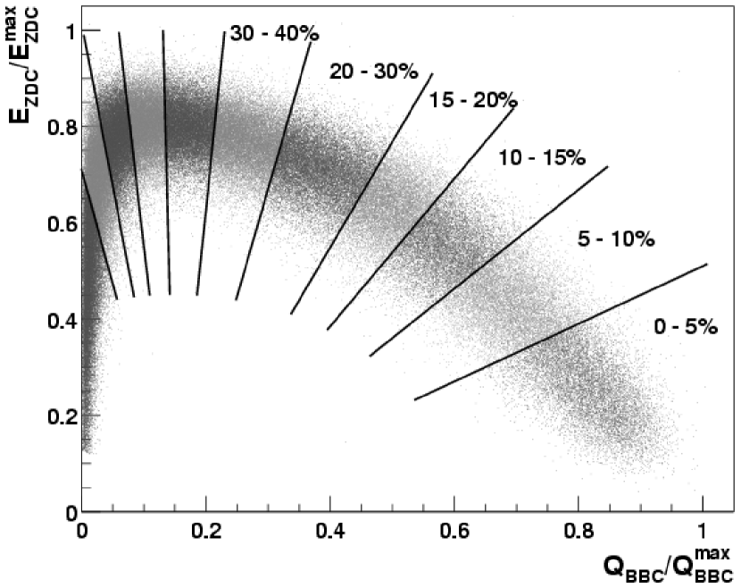
Refer to caption — Figure 1: BBC versus ZDC analog response. The lines represent the centrality cut boundaries.

For the present analysis, we use the PHENIX minimum bias trigger events, which are determined by a coincidence between north and south BBC signals. We also require a collision vertex within $\pm$ 30 cm from the center of the spectrometer. The collision vertex resolution determined by the BBC is about 6 mm in Au+Au collisions in minimum bias events PHENIX_inner . The PHENIX minimum bias trigger events include $92.2^{+2.5}_{-3.0}$ % of the 6.9 barn Au+Au total inelastic cross section PPG014 . Figure 1 shows the correlation between the BBC charge sum and ZDC total energy for Au+Au at $\sqrt{s_{NN}}$ = 200 GeV. The lines on the plot indicate the centrality definition in the analysis. For the centrality determination, these events are subdivided into 11 bins using the BBC and ZDC correlation: 0–5%, 5–10%, 10–15%, 15–20%, 20–30%, …, 70–80% and 80–92%. Due to the statistical limitations in the peripheral events, we also use the 60–92% centrality bin as the most peripheral bin. After event selection, we analyze 2.02 $\times 10^{7}$ minimum bias events, which represents $\sim$ 140 times more events than used in our published Au+Au data at 130 GeV PPG006 ; PPG009 . Based on a Glauber model calculation PPG009 ; PPG014 we use two global quantities to characterize the event centrality: the average number of participants $\langle N_{part}\rangle$ and the average number of collisions $\langle N_{coll}\rangle$ associated with each centrality bin (Table 1).

Table 1: The average nuclear overlap function (

\langle T_{\rm AuAu}\rangle

), the number of nucleon-nucleon binary collisions (

\langle N_{coll}\rangle

), and the number of participant nucleons (

\langle N_{part}\rangle

) obtained from a Glauber Monte Carlo PPG009 ; PPG014 correlated with the BBC and ZDC response for Au+Au at

\sqrt{s_{NN}}

= 200 GeV as a function of centrality. Centrality is expressed as percentiles of

\sigma_{\rm AuAu}

= 6.9 barn with 0% representing the most central collisions. The last line refers to minimum bias collisions.

Centrality	$\langle T_{\rm AuAu}\rangle$ (mb^-1)	$\langle N_{coll}\rangle$	$\langle N_{part}\rangle$
0- 5%	25.37 $\pm$ 1.77	1065.4 $\pm$ 105.3	351.4 $\pm$ 2.9
0-10%	22.75 $\pm$ 1.56	955.4 $\pm$ 93.6	325.2 $\pm$ 3.3
5-10%	20.13 $\pm$ 1.36	845.4 $\pm$ 82.1	299.0 $\pm$ 3.8
10-15%	16.01 $\pm$ 1.15	672.4 $\pm$ 66.8	253.9 $\pm$ 4.3
10-20%	14.35 $\pm$ 1.00	602.6 $\pm$ 59.3	234.6 $\pm$ 4.7
15-20%	12.68 $\pm$ 0.86	532.7 $\pm$ 52.1	215.3 $\pm$ 5.3
20-30%	8.90 $\pm$ 0.72	373.8 $\pm$ 39.6	166.6 $\pm$ 5.4
30-40%	5.23 $\pm$ 0.44	219.8 $\pm$ 22.6	114.2 $\pm$ 4.4
40-50%	2.86 $\pm$ 0.28	120.3 $\pm$ 13.7	74.4 $\pm$ 3.8
50-60%	1.45 $\pm$ 0.23	61.0 $\pm$ 9.9	45.5 $\pm$ 3.3
60-70%	0.68 $\pm$ 0.18	28.5 $\pm$ 7.6	25.7 $\pm$ 3.8
60-80%	0.49 $\pm$ 0.14	20.4 $\pm$ 5.9	19.5 $\pm$ 3.3
60-92%	0.35 $\pm$ 0.10	14.5 $\pm$ 4.0	14.5 $\pm$ 2.5
70-80%	0.30 $\pm$ 0.10	12.4 $\pm$ 4.2	13.4 $\pm$ 3.0
70-92%	0.20 $\pm$ 0.06	8.3 $\pm$ 2.4	9.5 $\pm$ 1.9
80-92%	0.12 $\pm$ 0.03	4.9 $\pm$ 1.2	6.3 $\pm$ 1.2
min. bias	6.14 $\pm$ 0.45	257.8 $\pm$ 25.4	109.1 $\pm$ 4.1

III.2 Track Selection

Charged particle tracks are reconstructed by the DC based on a combinatorial Hough transform PHENIX_recoNIM – which gives the angle of the track in the main bend plane. The main bend plane is perpendicular to the beam axis (azimuthal direction). PC1 is used to measure the position of the hit in the longitudinal direction (along the beam axis). When combined with the location of the collision vertex along the beam axis (from the BBC), the PC1 hit gives the polar angle of the track. Only tracks with valid information from both the DC and PC1 are used in the analysis. In order to associate a track with a hit on the TOF, the track is projected to its expected hit location on the TOF. Tracks are required to have a hit on the TOF within $\pm$ 2 $\sigma$ of the expected hit location in both the azimuthal and beam directions. Finally, a cut on the energy loss in the TOF scintillator is applied to each track. This $\beta$ -dependent energy loss cut is based on a parameterization of the Bethe-Bloch formula, i.e. $dE/dx\approx\beta^{-5/3}$ , where $\beta=L/(c\cdot t_{\rm TOF})$ , $L$ is the path-length of the track trajectory from the collision vertex to the hit position of the TOF wall, $t_{\rm TOF}$ is the time-of-flight, and $c$ is the speed of light. The flight path-length is calculated from a fit to the reconstructed track trajectory. The background due to random association of DC/PC1 tracks with TOF hits is reduced to a negligible level when the mass cut used for particle identification is applied (described in the next section).

III.3 Particle Identification

The charged particle identification (PID) is performed by using the combination of three measurements: time-of-flight from the BBC and TOF, momentum from the DC, and flight path-length from the collision vertex point to the hit position on the TOF wall. The square of the mass is derived from the following formula,

m^{2}=\frac{p^{2}}{c^{2}}\Bigl{[}{\Bigl{(}\frac{t_{\rm TOF}}{L/c}\Bigr{)}}^{2}-1\Bigr{]},

(1)

where $p$ is the momentum, $t_{\rm TOF}$ is the time-of-flight, $L$ is a flight path-length, and $c$ is the speed of light. The charged particle identification is performed using cuts in $m^{2}$ and momentum space.

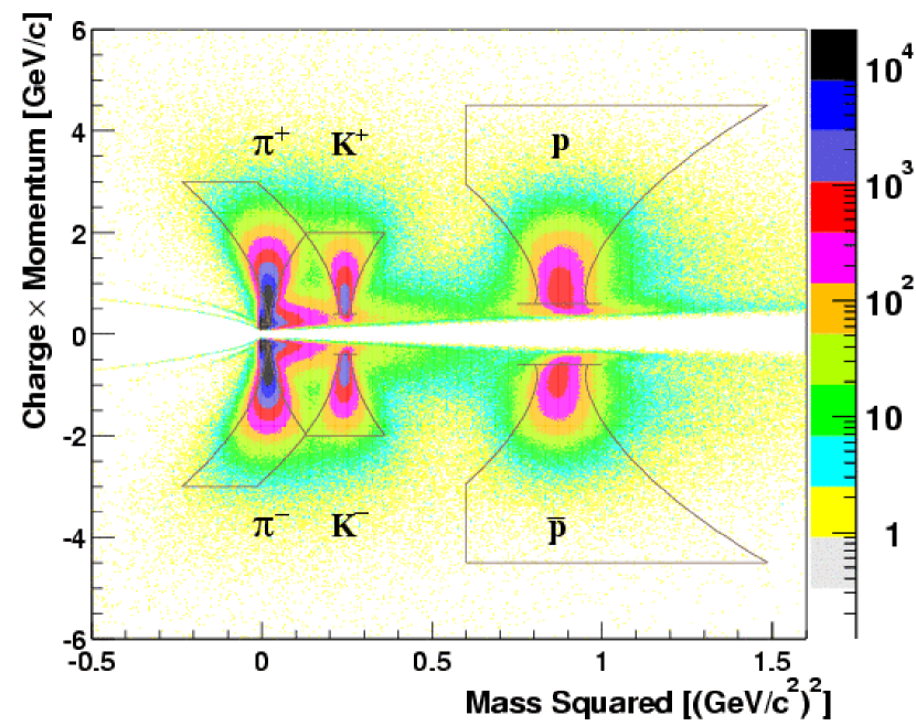
In Figure 2, a plot of $m^{2}$ versus momentum multiplied by charge is shown together with applied PID cuts as solid curves. We use 2 $\sigma$ standard deviation PID cuts in $m^{2}$ and momentum space for each particle species. The PID cut is based on a parameterization of the measured $m^{2}$ width as a function of momentum,

	$\displaystyle{\sigma^{2}_{m^{2}}}$	$\displaystyle=$	$\displaystyle\frac{\sigma_{\alpha}^{2}}{K_{1}^{2}}(4m^{4}p^{2})+\frac{\sigma_{ms}^{2}}{K_{1}^{2}}\Bigl{[}4m^{4}\Bigl{(}1+\frac{m^{2}}{p^{2}}\Bigr{)}\Bigl{]}$		(2)
		$\displaystyle+$	$\displaystyle\frac{\sigma_{t}^{2}c^{2}}{L^{2}}\bigl{[}4p^{2}\bigl{(}m^{2}+p^{2}\bigr{)}\bigr{]},$		(2)

where $\sigma_{\alpha}$ is the angular resolution, $\sigma_{ms}$ is the multiple scattering term, $\sigma_{t}$ is the overall time-of-flight resolution, $m$ is the centroid of $m^{2}$ distribution for each particle species, and $K_{1}$ is a magnetic field integral constant term of 87.0 mrad $\cdot$ GeV. The parameters for PID are, $\sigma_{\alpha}=0.835$ mrad, $\sigma_{ms}=0.86$ mrad $\cdot$ GeV and $\sigma_{t}=120$ ps. Through improvements in alignment and calibrations, the momentum resolution is improved over the 130 GeV data PPG009 . The centrality dependence of the width and the mean position of the $m^{2}$ distribution has also been checked. There is no clear difference seen between central and peripheral collisions. For pion identification above 2 GeV/ $c$ , we apply an asymmetric PID cut to reduce kaon contamination of the pions. As shown by the lines in Figure 2, the overlap region which is within the 2 $\sigma$ cuts for both pions and kaons is excluded. For kaons, the upper momentum cut-off is 2 GeV/ $c$ since the pion contamination level for kaons is $\approx$ 10% at that momentum. The upper momentum cut-off on the pions is $\mbox{$p_{T}$}=$ 3 GeV/ $c$ – where the kaon contamination reaches $\approx$ 10%. The contamination of protons by kaons reaches about 5% at 4 GeV/ $c$ . Electron (positron) and decay muon background at very low $p_{T}$ ( $<$ 0.3 GeV/ $c$ ) are well separated from the pion mass-squared peak. The contamination background on each particle species is not subtracted in the analysis. For protons, the upper momentum cut-off is set at 4.5 GeV/ $c$ due to statistical limitations and background at high $p_{T}$ . An additional cut on $m^{2}$ for protons and anti-protons, $m^{2}>$ 0.6 $({\rm GeV}/c^{2})^{2}$ , is introduced to reduce background. The lower momentum cut-offs are 0.2 GeV/ $c$ for pions, 0.4 GeV/ $c$ for kaons, and 0.6 GeV/ $c$ for $p$ and $\overline{p}$ . This cut-off value for $p$ and $\overline{p}$ is larger than those for pions and kaons due to the large energy loss effect.

III.4 Acceptance, Decay and Multiple Scattering Corrections

In order to correct for 1) the geometrical acceptance, 2) in-flight decay for pions and kaons, 3) the effect of multiple scattering, and 4) nuclear interactions with materials in the detector (including anti-proton absorption), we use PISA (PHENIX Integrated Simulation Application), a GEANT GEANT based Monte Carlo (MC) simulation program of the PHENIX detector. The single particle tracks are passed from GEANT through the PHENIX event reconstruction software PHENIX_recoNIM . In this simulation, the BBC, TOF, and DC detector responses are tuned to match the real data. For example, dead areas of DC and TOF are included, and momentum and time-of-flight resolution are tuned. The track association to TOF in both azimuth ( $\phi$ ) and along the beam axis ( $z$ ) as a function of momentum and the PID cut boundaries are parameterized to match the real data. A fiducial cut is applied to choose identical active areas on the TOF in both the simulation and data. We generate 1 $\times 10^{7}$ single particle events for each particle species ( $\pi^{\pm}$ , $K^{\pm}$ , $p$ and $\overline{p}$ ) with low $p_{T}$ enhanced ( $<$ 2 GeV/ $c$ ) + flat $p_{T}$ distributions for high $p_{T}$ (2 – 4 GeV/ $c$ for pions and kaons, 2 – 8 GeV/ $c$ for $p$ and $\overline{p}$ ) ¹¹1Due to the good momentum resolution at the high $p_{T}$ region, the momentum smearing effect for a steeply falling spectrum is $<$ 1% at $p_{T}$ = 5 GeV/ $c$ . The flat $p_{T}$ distribution up to 5 GeV/ $c$ can be used to obtain the correction factors.. The efficiencies are determined in each $p_{T}$ bin by dividing the reconstructed output by the generated input as expressed as follows:

\epsilon_{\rm acc}(j,\mbox{$p_{T}$})=\frac{\mbox{\rm\# of reconstructed MC tracks}}{\mbox{\rm\# of generated MC tracks}},

(3)

where $j$ is the particle species. The resulting correction factors (1/ $\epsilon_{\rm acc}$ ) are applied to the data in each $p_{T}$ bin and for each individual particle species.

III.5 Detector Occupancy Correction

Due to the high multiplicity environment in heavy ion collisions, which causes high occupancy and multiple hits on a detector cell such as scintillator slats of the TOF, it is expected that the track reconstruction efficiency in central events is lower than that in peripheral events. The typical occupancy at TOF is less than 10% in the most central Au+Au collisions. To correct for this effect, we merge single particle simulated events with real events and calculate the track reconstruction efficiency for each simulated track as follows:

\epsilon_{\rm mult}(i,j)=\frac{\mbox{\rm\# of reconstructed embedded tracks}}{\mbox{\rm\# of embedded tracks}},

(4)

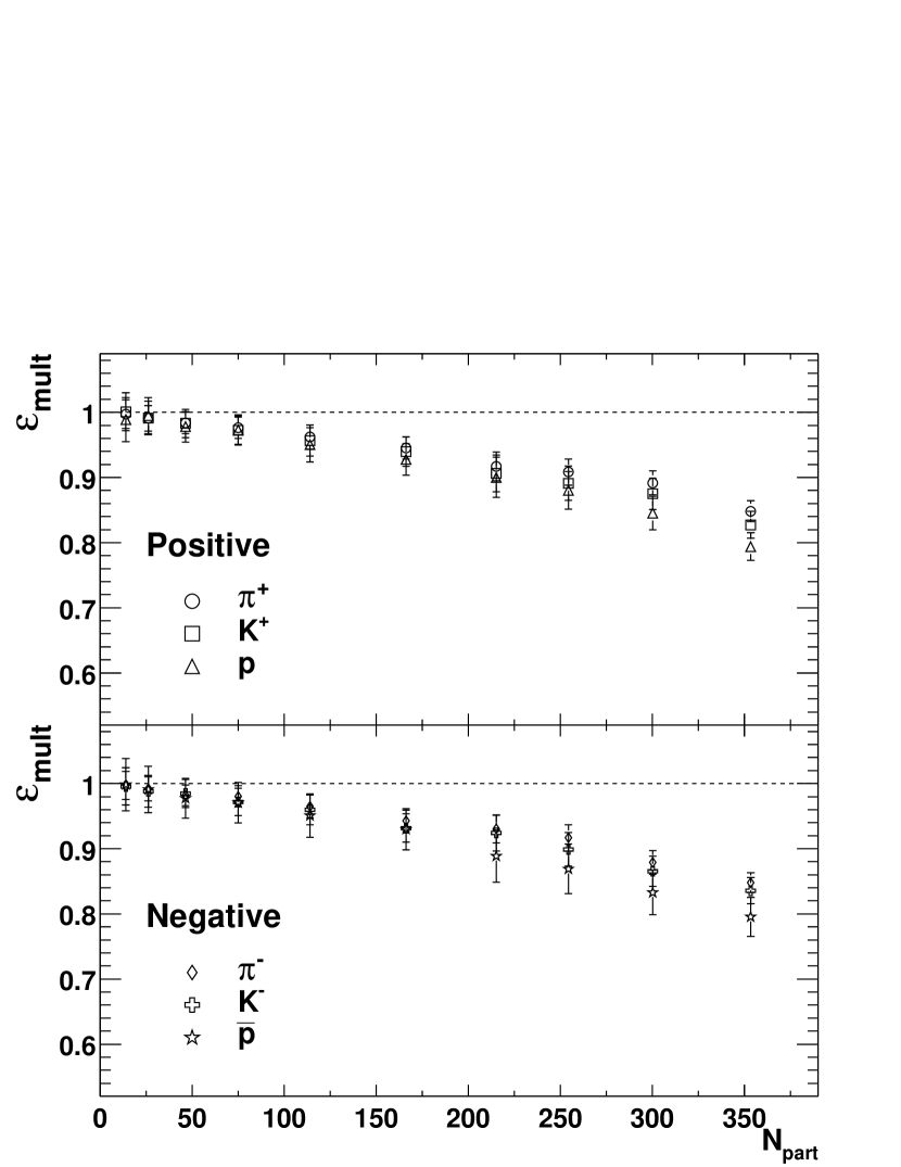
where $i$ is the centrality bins and $j$ is the particle species. This study has been performed for each particle species and each centrality bin. The track reconstruction efficiencies are factorized (into independent terms depending on centrality and $p_{T}$ ) for $\mbox{$p_{T}$}>0.4$ GeV/ $c$ , since there is no $p_{T}$ dependence in the efficiencies above that $p_{T}$ . Figure 3 shows the dependence of track reconstruction efficiency for $\pi^{\pm}$ , $K^{\pm}$ , $p$ and $\overline{p}$ as a function of centrality expressed as $N_{part}$ . The efficiency in the most central 0–5% events is about 80% for protons ( $\overline{p}$ ), 83% for kaons and 85% for pions. Slower particles are more likely lost due to high occupancy in the TOF because the system responds to the earliest hit. For the most peripheral 80–92% events, the efficiency for detector occupancy effect is $\approx$ 99% for all particle species. The factors are applied to the spectra for each particle species and centrality bin. Systematic uncertainties on detector occupancy corrections (1/ $\epsilon_{\rm mult}$ ) are less than 3%.

III.6 Weak Decay Correction

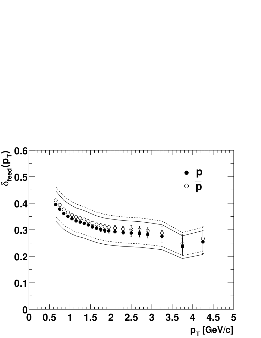
Protons and anti-protons from weak decays (e.g. from $\Lambda$ and $\overline{\Lambda}$ ) can be reconstructed as tracks in the PHENIX spectrometer. The proton and anti-proton spectra are corrected to remove the feed-down contribution from weak decays using a HIJING HIJING simulation. HIJING output has been tuned to reproduce the measured particle ratios of $\Lambda/p$ and $\mbox{$\overline{\Lambda}$}/\mbox{$\overline{p}$}$ along with their $p_{T}$ dependencies in $\sqrt{s_{NN}}$ = 130 GeV Au+Au collisions PPG012 which include contribution from $\Xi$ and $\Sigma^{0}$ . Corrections for feed-down from $\Sigma^{\pm}$ are not applied, as these yields were not measured. About 2 $\times 10^{6}$ central HIJING events (impact parameter $b=0-3$ fm) covering the TOF acceptance have been generated and processed through the PHENIX reconstruction software. To calculate the feed-down corrections, the $\mbox{$\overline{p}$}/p$ and $\mbox{$\overline{\Lambda}$}/\Lambda$ yield ratios were assumed to be independent of $p_{T}$ and centrality. The systematic error due to the feed-down correction is estimated at 6% by varying the $\Lambda/p$ and $\mbox{$\overline{\Lambda}$}/\mbox{$\overline{p}$}$ ratios within the systematic errors of the $\mbox{$\sqrt{s_{NN}}$}=$ 130 GeV Au+Au measurement PPG012 ( $\pm$ 24%) and assuming $m_{T}$ -scaling at high $p_{T}$ . This uncertainty could be larger if the $\Lambda/p$ and $\mbox{$\overline{\Lambda}$}/\mbox{$\overline{p}$}$ ratios change significantly with $p_{T}$ and beam energy. The fractional contribution to the $p$ ( $\overline{p}$ ) yield from $\Lambda(\mbox{$\overline{\Lambda}$})$ , $\delta_{\rm feed}(\mbox{$p_{T}$})$ , is shown in Figure 4. The solid (dashed) lines represent the systematic errors for protons ( $\overline{p}$ ). The obtained factor is about 40% below 1 GeV/ $c$ and 30% at 4 GeV/ $c$ . We multiply the proton and anti-proton spectra by the factor, $C_{\rm feed}$ , for all centrality bins as a function of $p_{T}$ :

C_{\rm feed}(j,\mbox{$p_{T}$})=1-\delta_{\rm feed}(j,\mbox{$p_{T}$}),

(5)

where $j=p,\mbox{$\overline{p}$}$ .

III.7 Invariant Yield

Applying the data cuts and corrections discussed above, the final invariant yield for each particle species and centrality bin are derived using the following equation.

\frac{1}{2\pi\mbox{$p_{T}$}}\frac{d^{2}N}{dp_{T}dy}=\frac{1}{2\pi\mbox{$p_{T}$}}\cdot\frac{1}{N_{evt}(i)}\cdot C_{ij}(\mbox{$p_{T}$})\cdot\frac{N_{j}(i,\mbox{$p_{T}$})}{\Delta\mbox{$p_{T}$}\Delta y},

(6)

where $y$ is rapidity, $N_{evt}(i)$ is the number of events in each centrality bin $i$ , $C_{ij}(\mbox{$p_{T}$})$ is the total correction factor and $N_{j}(i,\mbox{$p_{T}$})$ is the number of counts in each centrality bin $i$ , particle species $j$ , and $p_{T}$ . The total correction factor is composed of:

C_{ij}(\mbox{$p_{T}$})=\frac{1}{\epsilon_{\rm acc}(j,\mbox{$p_{T}$})}\cdot\frac{1}{\epsilon_{\rm mult}(i,j)}\cdot C_{\rm feed}(j,\mbox{$p_{T}$}).

(7)

III.8 Systematic Uncertainties

To estimate systematic uncertainties on the $p_{T}$ distribution and particle ratios, various sets of $p_{T}$ spectra and particle ratios were made by changing the cut parameters including the fiducial cut, PID cut, and track association windows slightly from what was used in the analysis. For each of these spectra and ratios using modified cuts, the same changes in the cuts were made in the Monte Carlo analysis. The absolutely normalized spectra with different cut conditions are divided by the spectra with the baseline cut conditions, resulting in uncertainties associated with each cut condition as a function of $p_{T}$ . The various uncertainties are added in quadrature. Three different centrality bins (minimum bias, central 0–5%, and peripheral 60–92%) are used to study the centrality dependence of systematic errors. The same procedure has been applied for the following particle ratios: $\pi^{-}/\pi^{+}$ , $K^{-}/K^{+}$ , $\mbox{$\overline{p}$}/p$ , $K/\pi$ , $p/\pi^{+}$ , and $\mbox{$\overline{p}$}/\pi^{-}$ .

Table 2 shows the systematic errors of the $p_{T}$ spectra for central collisions. The systematic uncertainty on the absolute value of momentum (momentum scale) are estimated as 3% in the measured $p_{T}$ range by comparing the known proton mass to the value measured as protons in real data. It is found that the total systematic error on the $p_{T}$ spectra is 8–14% in both central and peripheral collisions. For the particle ratios, the typical systematic error is about 6% for all particle species. The dominant source of uncertainties on the central-to-peripheral ratio scaled by $N_{coll}$ ( $R_{CP}$ ) are the systematic errors on the nuclear overlap function, $T_{\rm AuAu}$ (see Table 3). The systematic errors on $dN/dy$ and $\langle p_{T}\rangle$ are discussed in Section IV.3 together with the procedure for the determination of these quantities.

IV RESULTS

In this section, the $p_{T}$ and transverse mass spectra and yields of identified charged hadrons as a function of centrality are shown. Also a systematic study of particle ratios in Au+Au collisions at $\sqrt{s_{NN}}$ = 200 GeV at mid-rapidity is presented.

IV.1 Transverse Momentum Distributions

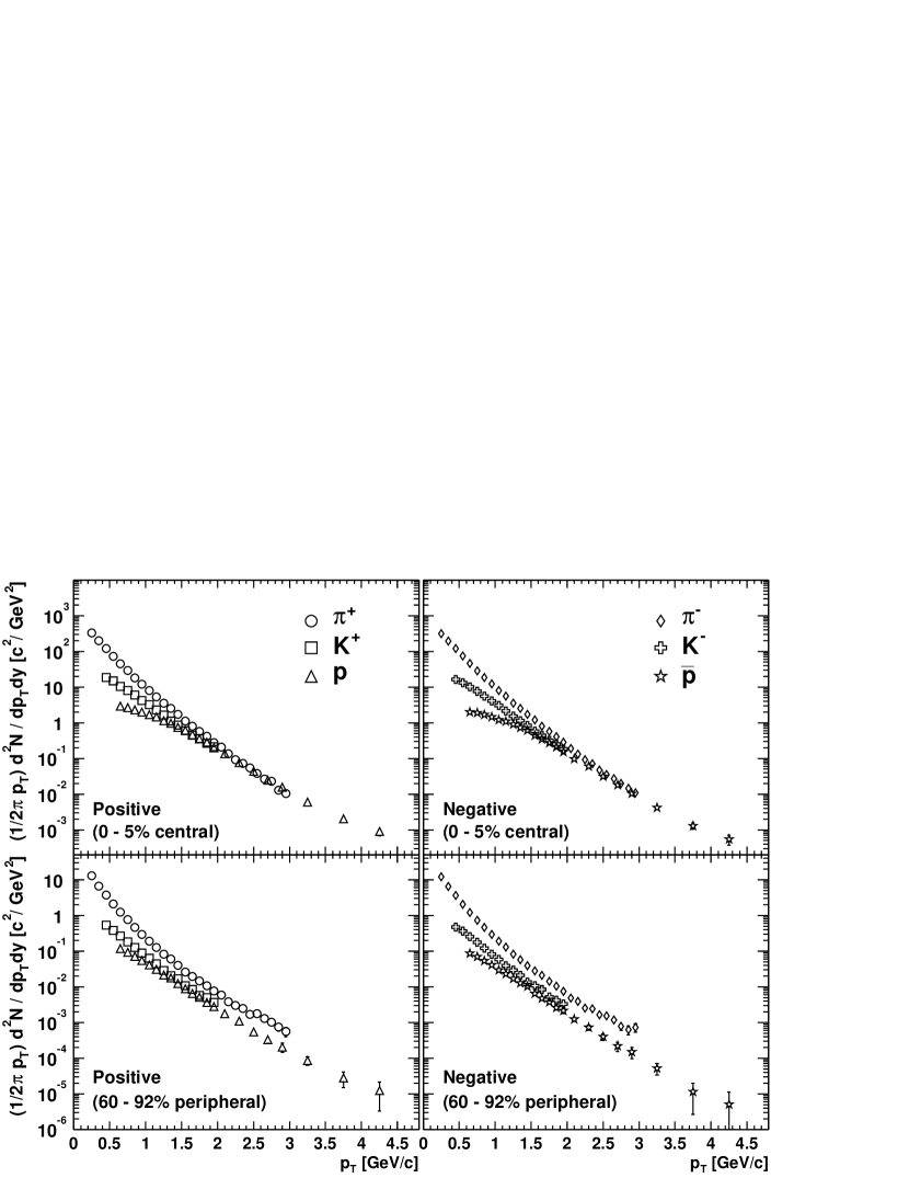
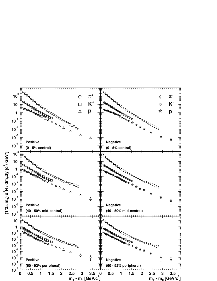
Figure 5 shows the $p_{T}$ distributions for pions, kaons, protons, and anti-protons. The top two plots are for the most central 0–5% collisions, and the bottom two are for the most peripheral 60–92% collisions. The spectra for positive particles are presented on the left, and those for negative particles on the right. For $\mbox{$p_{T}$}<$ 1.5 GeV/ $c$ in central events, the data show a clear mass dependence in the shapes of the spectra. The $p$ and $\overline{p}$ spectra have a shoulder-arm shape, the pion spectra have a concave shape, and the kaons fall exponentially. On the other hand, in the peripheral events, the mass dependences of the $p_{T}$ spectra are less pronounced and the $p_{T}$ spectra are more nearly parallel to each other. Another notable observation is that at $p_{T}$ above $\approx$ 2.0 GeV/ $c$ in central events, the $p$ and $\overline{p}$ yields become comparable to the pion yields, which is also observed in 130 GeV Au+Au collisions PPG006 . This observation shows that a significant fraction of the total particle yield at $\mbox{$p_{T}$}\approx$ 2.0 – 4.5 GeV/ $c$ in Au+Au central collisions consists of $p$ and $\overline{p}$ .

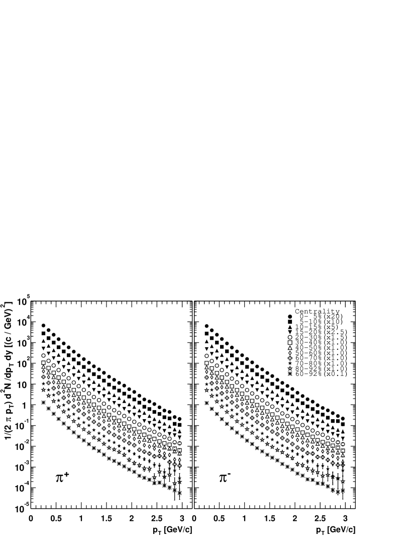
These high statistics Au+Au data at $\sqrt{s_{NN}}$ = 200 GeV allow us to perform a detailed study of the centrality dependence of the $p_{T}$ spectra. In this analysis, we use the eleven centrality bins described in Section III.1 as well as the combined peripheral bin (60–92%) for each particle species. Figure 6 shows the centrality dependence of the $p_{T}$ spectrum for $\pi^{+}$ (left) and $\pi^{-}$ (right). For clarity, the data points are scaled vertically as quoted in the figures. The error bars are statistical only. The pion spectra show an approximately power-law shape for all centrality bins. The spectra become steeper (fall faster with increasing $p_{T}$ ) for more peripheral collisions.

Table 2: Systematic errors on the

p_{T}

spectra for central events. All errors are given in percent.

	$\pi^{+}$	$\pi^{-}$	$K^{+}$	$K^{-}$	$p$		$\overline{p}$
$p_{T}$ range (GeV/ $c$ )	0.2 - 3.0	0.2 - 3.0	0.4 - 2.0	0.4 - 2.0	0.6 - 3.0	3.0 - 4.5	0.6 - 3.0	3.0 - 4.5
Cuts	6.2	6.2	11.2	9.5	6.6	11.6	6.6	11.6
Momentum scale	3	3	3	3	3	3	3	3
Occupancy correction	2	2	3	3	3	3	3	3
Feed-down correction	-	-	-	-	6.0	6.0	6.0	6.0
Total	7.2	7.2	12.0	10.4	9.9	13.7	9.9	9.9

Table 3: Systematic errors on Central-to-Peripheral ratio (

R_{CP}

). All errors are given in percent.

Source	$(\pi^{+}+\pi^{-})/2$	$(K^{+}+K^{-})/2$	$(p+\mbox{$\overline{p}$})/2$
Occupancy correction (central)	2	3	3
Occupancy correction (peripheral)	2	3	3
$\langle T_{\rm AuAu}\rangle$ (0–10%)	6.9	6.9	6.9
$\langle T_{\rm AuAu}\rangle$ (60–92%)	28.6	28.6	28.6
Total	29.5	29.7	29.7

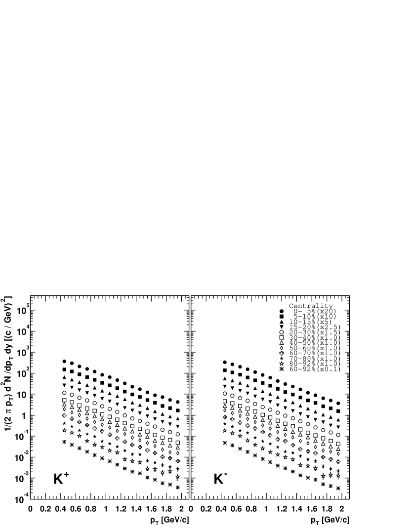
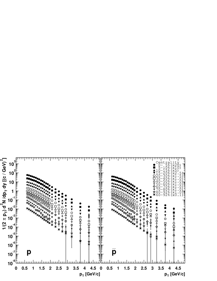
Figure 7 shows similar plots for kaons. The data can be well approximated by an exponential function in $p_{T}$ for all centralities. Finally, the centrality dependence of the $p_{T}$ spectra for protons (left) and anti-protons (right) is shown in Figure 8. As in Figure 5, both $p$ and $\overline{p}$ spectra show a strong centrality dependence below 1.5 GeV/ $c$ , i.e. they develop a shoulder at low $p_{T}$ and the spectra flatten (fall more slowly with increasing $p_{T}$ ) with increasing collision centrality.

Up to $\mbox{$p_{T}$}=1.5\sim 2$ GeV/ $c$ , it has been found that hydrodynamic models can reproduce the data well for $\pi^{\pm}$ , $K^{\pm}$ , $p$ and $\overline{p}$ spectra at 130 GeV PPG009 , and also the preliminary data at 200 GeV in Au+Au collisions (e.g. hydro_2 ; hydro_200gev ). These models assume thermal equilibrium and that the created particles are affected by a common transverse flow velocity $\beta_{T}$ and freeze-out (stop interacting) at a temperature $T_{fo}$ with a fixed initial condition governed by the equation of state (EOS) of matter. There are several types of hydrodynamic calculations, e.g., (1) a conventional hydrodynamic fit to the experimental data with two free parameters, $\beta_{T}$ and $T_{fo}$ Schnedermann , (2) a combination of hydrodynamics and a hadronic cascade model hydro_2 , (3) transverse and longitudinal flow with simultaneous chemical and thermal freeze-outs within the statistical thermal model hydro_3 , (4) requiring the early thermalization with a QGP type EOS Heinz . Despite the differences between the hydrodynamic models, all models are in qualitative agreement with the identified single particle spectra in central collisions at low $p_{T}$ as seen in reference PPG009 . However, they fail to reproduce the peripheral spectra above $\mbox{$p_{T}$}\simeq 1$ GeV/ $c$ and their applicability in the high $p_{T}$ region ( $>$ 2 GeV/ $c$ ) is limited. Comparison with the detailed centrality dependence of hadron spectra presented here would shed light on further understanding of the EOS, chemical properties in the model, and the freeze-out conditions at RHIC.

IV.2 Transverse Mass Distributions

In order to quantify the observed particle mass dependence of the $p_{T}$ spectra shape and their centrality dependence, the transverse mass spectra for identified charged hadrons are presented here. From former studies at lower beam energies, it is known that the invariant differential cross sections in $p+p$ , $p+A$ , and $A+A$ collisions generally show a shape of an exponential in $m_{T}-m_{0}$ , where $m_{0}$ is particle mass, and $m_{T}=\sqrt{p_{T}^{2}+m_{0}^{2}}$ is transverse mass. For an $m_{T}$ spectrum with an exponential shape, one can parameterize it as follows:

\frac{d^{2}N}{2\pi m_{T}dm_{T}dy}=\frac{1}{2\pi T(T+m_{0})}\cdot A\cdot\exp{(-\frac{m_{T}-m_{0}}{T})},

(8)

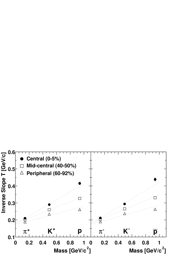
where $T$ is referred to as the inverse slope parameter, and $A$ is a normalization parameter which contains information on $dN/dy$ . In Figure 9, $m_{T}$ distributions for $\pi^{\pm}$ , $K^{\pm}$ , $p$ and $\overline{p}$ for central 0–5% (top panels), mid-central 40–50% (middle panels) and peripheral 60–92% (bottom panels) collisions are shown. The spectra for positive particles are on the left and for negative particles are on the right. The solid lines overlaid on each spectra are the fit results using Eq. 8. The error bars are statistical only. As seen in Figure 9, all the $m_{T}$ spectra display an exponential shape in the low $m_{T}$ region. However, at higher $m_{T}$ , the spectra become less steep, which corresponds to a power-law behavior in $p_{T}$ . Thus, the inverse slope parameter in Eq. 8 depends on the fitting range. In this analysis, the fits cover the range 0.2 – 1.0 GeV/ $c^{2}$ for pions and 0.1 – 1.0 GeV/ $c^{2}$ for kaons, protons, and anti-protons in $m_{T}-m_{0}$ . The low $m_{T}$ region ( $m_{T}-m_{0}<$ 0.2 GeV/ $c^{2}$ ) for pions is excluded from the fit to eliminate the contributions from resonance decays. The inverse slope parameters for each particle species in the three centrality bins are summarized in Figure 10 and in Table 4. The inverse slope parameters increase with increasing particle mass in all centrality bins. This increase for central collisions is more rapid for heavier particles.

Such a behavior was derived, under certain conditions, by E. Schnedermann et al. Schnedermann1994 for central collisions and by T. Csörgő et al. Csorgo for non-central heavy ion collisions:

T=T_{0}+m\mbox{$\langle u_{t}\rangle$}^{2}.

(9)

Here $T_{0}$ is a freeze-out temperature and $\langle u_{t}\rangle$ is a measure of the strength of the (average radial) transverse flow. The dotted lines in Figure 10 represent a linear fit of the results from each centrality bin as a function of mass using Eq. 9. The fit parameters for positive and negative particles are shown in Table 4. It indicates, that the linear extrapolation of the slope parameter $T(m)$ to zero mass has the same intercept parameters $T_{0}$ in all the centrality classes, indicating that the freeze-out temperature is approximately independent of the centrality. On the other hand, $\langle u_{t}\rangle$ , the strength of the average transverse flow is increasing with increasing centrality, supporting the hydrodynamic picture.

Motivated by the idea of a Color Glass Condensate, the authors of reference mt_scaling argued that the $m_{T}$ spectra (not $\mbox{$m_{T}$}-m_{0}$ ) of identified hadrons at RHIC energy follow a generalized scaling law for all centrality classes when the proton (kaon) spectrum is multiplied by a factor of 0.5 (2.0). The 200 GeV Au+Au pion and kaon spectra seem to follow this $m_{T}$ scaling, but proton and anti-proton spectra are below it by a factor of $\sim$ 2 for all centralities. Since $p$ and $\overline{p}$ spectra presented here are corrected for weak decays from $\Lambda$ and $\overline{\Lambda}$ , the model also needs to study the feed-down effect to conclude that a universal $m_{T}$ scaling law is seen at RHIC.

Table 4: (Top) Inverse slope parameters for

\pi

K

p

and

\overline{p}

for the 0–5%, 40–50% and 60–92% centrality bins, in units of MeV/

c^{2}

. The errors are statistical only. (Bottom) The extracted fit parameters of the freeze-out temperature (

T_{0}

) in units of MeV/

c^{2}

and the measure of the strength of the average radial transverse flow (

\langle u_{t}\rangle

) using Eq. 9. The fit results shown here are for positive and negative particles, as denoted in the superscripts, and for three different centrality bins.

Particle	0–5%	40–50%	60–92%
$\pi^{+}$	210.2 $\pm$ 0.8	201.9 $\pm$ 0.8	187.8 $\pm$ 0.7
$\pi^{-}$	211.9 $\pm$ 0.7	203.0 $\pm$ 0.7	189.2 $\pm$ 0.7
$K^{+}$	290.2 $\pm$ 2.2	260.6 $\pm$ 2.4	233.9 $\pm$ 2.6
$K^{-}$	293.8 $\pm$ 2.2	265.1 $\pm$ 2.3	237.4 $\pm$ 2.6
$p$	414.8 $\pm$ 7.5	326.3 $\pm$ 5.9	260.7 $\pm$ 5.4
$\overline{p}$	437.9 $\pm$ 8.5	330.5 $\pm$ 6.4	262.1 $\pm$ 5.9
Fit parameter	0–5%	40–50%	60–92%
$T_{0}^{(+)}$	177.0 $\pm$ 1.2	179.5 $\pm$ 1.2	173.1 $\pm$ 1.2
$T_{0}^{(-)}$	177.3 $\pm$ 1.2	179.6 $\pm$ 1.2	173.7 $\pm$ 1.1
$\mbox{$\langle u_{t}\rangle$}^{(+)}$	0.48 $\pm$ 0.07	0.40 $\pm$ 0.07	0.32 $\pm$ 0.07
$\mbox{$\langle u_{t}\rangle$}^{(-)}$	0.49 $\pm$ 0.07	0.41 $\pm$ 0.07	0.33 $\pm$ 0.07

IV.3 Mean Transverse Momentum and Particle Yields versus $N_{part}$

By integrating a measured $p_{T}$ spectrum over $p_{T}$ , one can determine the mean transverse momentum, $\langle p_{T}\rangle$ , and particle yield per unit rapidity, $dN/dy$ , for each particle species. The procedure to determine the mean $p_{T}$ and $dN/dy$ is described below: (1) Determine $dN/dy$ and $\langle p_{T}\rangle$ by integrating over the measured $p_{T}$ range from the data. (2) Fit several appropriate functional forms (detailed below) to the $p_{T}$ spectra. Note that all of the fits are reasonable approximations to the data. Integrate from zero to the first data point and from the last data point to infinity. (3) Sum the data yield and the two functional yield pieces together to get $dN/dy$ and $\langle p_{T}\rangle$ in each functional form. (4) Take the average between the upper and lower bounds from the different functional forms to obtain the final $dN/dy$ and $\langle p_{T}\rangle$ . The statistical uncertainties are determined from the data. The systematic errors from the extrapolation of yield are defined as half of the difference between the upper and lower bounds. (5) Determine the final systematic errors on $dN/dy$ and $\langle p_{T}\rangle$ for each centrality bin by taking the quadrature sum of the extrapolation errors, errors associated with cuts, detector occupancy corrections (for $dN/dy$ ) and feed-down corrections (for $p$ and $\overline{p}$ ).

For the extrapolation of $dN/dy$ and $\langle p_{T}\rangle$ , the following functional forms are used for different particle species: a power-law function and a $p_{T}$ exponential for pions, a $p_{T}$ exponential and an $m_{T}$ exponential for kaons, and a Boltzmann function, $p_{T}$ exponential, and $m_{T}$ exponential for protons and anti-protons. The effects of contamination background at high $p_{T}$ region for both $dN/dy$ and $\langle p_{T}\rangle$ are estimated as less than 1% for all particle species. The overall systematic uncertainties on both $dN/dy$ and $\langle p_{T}\rangle$ are about 10–15%. See Table 5 for the systematic errors of $dN/dy$ and Table 6 for those of $\langle p_{T}\rangle$ .

Table 5: Systematic errors on

dN/dy

for central 0–5% (top) and peripheral 60–92% (bottom) collisions. All errors are given in percent.

Source	$\pi^{+}$	$\pi^{-}$	$K^{+}$	$K^{-}$	$p$	$\overline{p}$
	Central 0–5%
Cuts + occupancy	6.5	6.5	11.6	10.0	7.2	7.2
Extrapolation	5.4	4.8	5.7	5.6	9.6	9.2
Contamination background	$<$ 1	$<$ 1	$<$ 1	$<$ 1	$<$ 1	$<$ 1
Feed-down	-	-	-	-	8.0	8.0
Total	8.4	8.0	12.9	11.4	14.4	14.4
	Peripheral 60–92%
Cuts + occupancy	6.5	6.5	8.3	7.2	8.3	8.3
Extrapolation	8.4	8.0	7.4	7.5	13.6	13.6
Contamination background	$<$ 1	$<$ 1	$<$ 1	$<$ 1	$<$ 1	$<$ 1
Feed-down	-	-	-	-	8.0	8.0
Total	10.6	10.3	11.1	10.3	17.8	17.8

Table 6: Systematic errors on

\langle p_{T}\rangle

for central 0–5% (top) and peripheral 60–92% (bottom) collisions. All errors are given in percent.

Source	$\pi^{+}$	$\pi^{-}$	$K^{+}$	$K^{-}$	$p$	$\overline{p}$
	Central 0–5%
Cuts	6.2	6.2	11.2	9.5	6.6	6.6
Extrapolation	3.9	3.5	3.5	3.3	6.2	5.9
Contamination background	$<$ 1	$<$ 1	$<$ 1	$<$ 1	$<$ 1	$<$ 1
Feed-down	-	-	-	-	1.0	1.0
Total	7.3	7.1	13.5	10.0	9.1	8.9
	Peripheral 60–92%
Cuts	6.2	6.2	7.7	6.6	7.7	7.7
Extrapolation	5.4	5.3	4.6	4.4	8.6	8.6
Contamination background	$<$ 1	$<$ 1	$<$ 1	$<$ 1	$<$ 1	$<$ 1
Feed-down	-	-	-	-	1.0	1.0
Total	8.2	8.1	8.9	7.9	11.5	11.5

Table 7: Centrality dependence of

\langle p_{T}\rangle

for

\pi^{\pm}

K^{\pm}

p

and

\overline{p}

in MeV/

c

. The errors are systematic only. The statistical errors are negligible.

$N_{part}$	$\pi^{+}$	$\pi^{-}$	$K^{+}$	$K^{-}$	$p$	$\overline{p}$
351.4	451 $\pm$ 33	455 $\pm$ 32	670 $\pm$ 78	677 $\pm$ 68	949 $\pm$ 85	959 $\pm$ 84
299.0	450 $\pm$ 33	454 $\pm$ 33	672 $\pm$ 78	679 $\pm$ 68	948 $\pm$ 84	951 $\pm$ 83
253.9	448 $\pm$ 33	453 $\pm$ 33	668 $\pm$ 78	676 $\pm$ 68	942 $\pm$ 84	950 $\pm$ 83
215.3	447 $\pm$ 34	449 $\pm$ 33	667 $\pm$ 78	670 $\pm$ 67	937 $\pm$ 84	940 $\pm$ 83
166.6	444 $\pm$ 35	447 $\pm$ 34	661 $\pm$ 77	668 $\pm$ 67	923 $\pm$ 85	920 $\pm$ 83
114.2	436 $\pm$ 35	440 $\pm$ 35	655 $\pm$ 77	654 $\pm$ 66	901 $\pm$ 83	892 $\pm$ 82
74.4	426 $\pm$ 35	429 $\pm$ 35	636 $\pm$ 54	644 $\pm$ 48	868 $\pm$ 88	864 $\pm$ 88
45.5	412 $\pm$ 35	416 $\pm$ 34	617 $\pm$ 53	621 $\pm$ 47	833 $\pm$ 86	824 $\pm$ 86
25.7	398 $\pm$ 34	403 $\pm$ 33	600 $\pm$ 52	606 $\pm$ 46	788 $\pm$ 84	777 $\pm$ 83
13.4	381 $\pm$ 32	385 $\pm$ 32	581 $\pm$ 51	579 $\pm$ 46	755 $\pm$ 82	747 $\pm$ 80
6.3	367 $\pm$ 30	371 $\pm$ 30	568 $\pm$ 51	565 $\pm$ 45	685 $\pm$ 78	708 $\pm$ 81

Table 8: Centrality dependence of

dN/dy

for

\pi^{\pm}

K^{\pm}

p

and

\overline{p}

. The errors are systematic only. The statistical errors are negligible.

$N_{part}$	$\pi^{+}$	$\pi^{-}$	$K^{+}$	$K^{-}$	$p$	$\overline{p}$
351.4	286.4 $\pm$ 24.2	281.8 $\pm$ 22.8	48.9 $\pm$ 6.3	45.7 $\pm$ 5.2	18.4 $\pm$ 2.6	13.5 $\pm$ 1.8
299.0	239.6 $\pm$ 20.5	238.9 $\pm$ 19.8	40.1 $\pm$ 5.1	37.8 $\pm$ 4.3	15.3 $\pm$ 2.1	11.4 $\pm$ 1.5
253.9	204.6 $\pm$ 18.0	198.2 $\pm$ 16.7	33.7 $\pm$ 4.3	31.1 $\pm$ 3.5	12.8 $\pm$ 1.8	9.5 $\pm$ 1.3
215.3	173.8 $\pm$ 15.6	167.4 $\pm$ 14.4	27.9 $\pm$ 3.6	25.8 $\pm$ 2.9	10.6 $\pm$ 1.5	7.9 $\pm$ 1.1
166.6	130.3 $\pm$ 12.4	127.3 $\pm$ 11.6	20.6 $\pm$ 2.6	19.1 $\pm$ 2.2	8.1 $\pm$ 1.1	5.9 $\pm$ 0.8
114.2	87.0 $\pm$ 8.6	84.4 $\pm$ 8.0	13.2 $\pm$ 1.7	12.3 $\pm$ 1.4	5.3 $\pm$ 0.7	3.9 $\pm$ 0.5
74.4	54.9 $\pm$ 5.6	52.9 $\pm$ 5.2	8.0 $\pm$ 0.8	7.4 $\pm$ 0.6	3.2 $\pm$ 0.5	2.4 $\pm$ 0.3
45.5	32.4 $\pm$ 3.4	31.3 $\pm$ 3.1	4.5 $\pm$ 0.4	4.1 $\pm$ 0.4	1.8 $\pm$ 0.3	1.4 $\pm$ 0.2
25.7	17.0 $\pm$ 1.8	16.3 $\pm$ 1.6	2.2 $\pm$ 0.2	2.0 $\pm$ 0.1	0.93 $\pm$ 0.15	0.71 $\pm$ 0.12
13.4	7.9 $\pm$ 0.8	7.7 $\pm$ 0.7	0.89 $\pm$ 0.09	0.88 $\pm$ 0.09	0.40 $\pm$ 0.07	0.29 $\pm$ 0.05
6.3	4.0 $\pm$ 0.4	3.9 $\pm$ 0.3	0.44 $\pm$ 0.04	0.42 $\pm$ 0.04	0.21 $\pm$ 0.04	0.15 $\pm$ 0.02

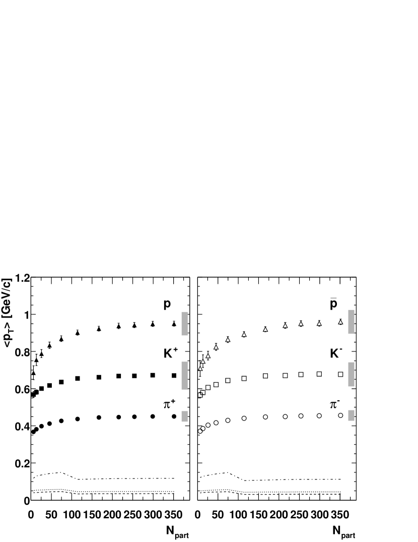
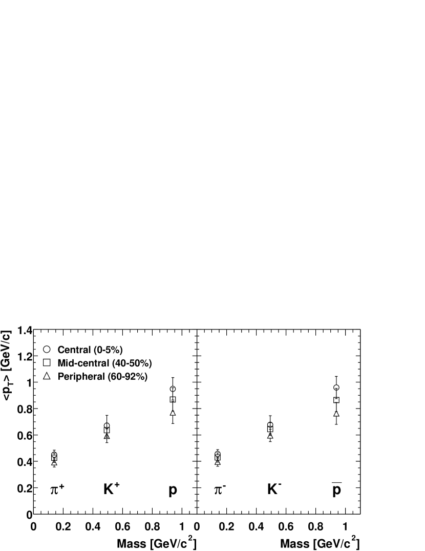
In Figure 11, the centrality dependence of $\langle p_{T}\rangle$ for $\pi^{\pm}$ , $K^{\pm}$ , $p$ and $\overline{p}$ is shown. The error bars in the figure represent the statistical errors. The systematic errors from cuts conditions are shown as shaded boxes on the right for each particle species. The systematic errors from extrapolations, which are scaled by a factor of 2 for clarity, are shown in the bottom for each particle species. The data are also summarized in Table 7. It is found that $\langle p_{T}\rangle$ for all particle species increases from the most peripheral to mid-central collisions, and appears to saturate from the mid-central to central collisions (although the $\langle p_{T}\rangle$ values for $p$ and $\overline{p}$ may continue to rise). It should be noted that while the total systematic errors on $\langle p_{T}\rangle$ listed in Table 6 is large, the trend shown in the figure is significant. One of the main sources of the uncertainty is the yield extrapolation in unmeasured $p_{T}$ range (e.g. $\mbox{$p_{T}$}<$ 0.6 GeV/ $c$ for protons and anti-protons). These systematic errors are correlated, and therefore move the curve up and down simultaneously. In Figure 12, the particle mass and centrality dependence of $\langle p_{T}\rangle$ are shown. The data presented here are the $\langle p_{T}\rangle$ for the 0–5%, 40–50% and 60–92% centrality bins. Figure 12 is similar to Figure 10, which shows the inverse slope parameters, in that the $\langle p_{T}\rangle$ increases with particle mass and with centrality. This is qualitatively consistent with the hydrodynamic expansion picture hydro_200gev ; Schnedermann1994 ; Csorgo .

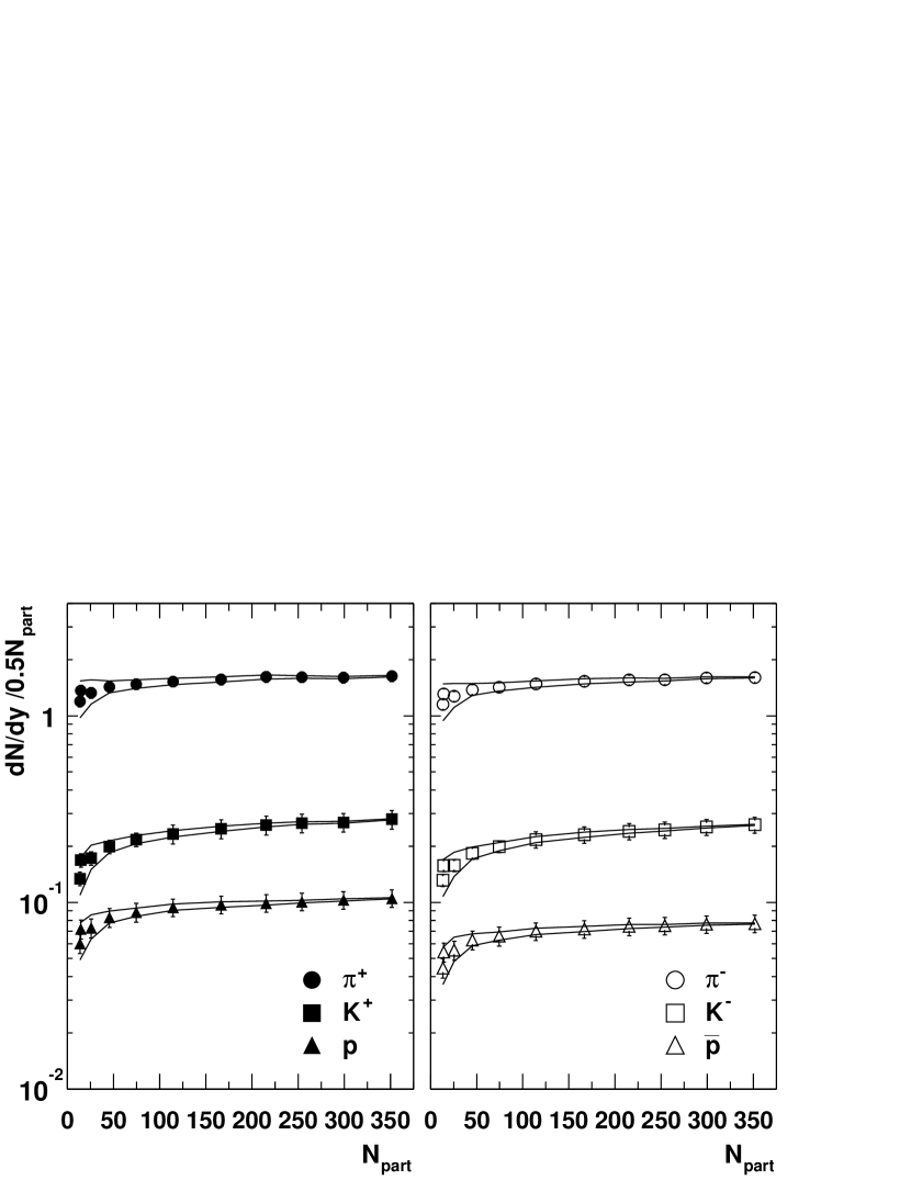
Figure 13 shows the centrality dependence of $dN/dy$ per participant pair (0.5 $N_{part}$ ). The data are summarized in Table 8. The error bars on each point represent the quadratic sum of the statistical errors and systematic errors from cut conditions. The statistical errors are negligible. The lines represent the effect of the systematic error on $N_{part}$ which affects all curves in the same way. The data indicate that $dN/dy$ per participant pair increases for all particle species with $N_{part}$ up to $\approx$ 100, and saturates from the mid-central to the most central collisions. From $dN/dy$ for protons and anti-protons, we obtain the net proton number at mid-rapidity for the most central 0–5% collisions, $dN/dy|_{p}-dN/dy|_{\mbox{$\overline{p}$}}=18.47-13.52=4.95\pm 2.74$ , which is consistent with the preliminary result at 200 GeV Au+Au (mid-rapidity) reported by the BRAHMS collaboration BRAHMS_200_netproton .

IV.4 Particle Ratios

The ratios of $\pi^{-}/\pi^{+}$ , $K^{-}/K^{+}$ , $p/\mbox{$\overline{p}$}$ , $K/\pi$ , $p/\pi$ and $\mbox{$\overline{p}$}/\pi$ measured as a function of $p_{T}$ and centrality at $\mbox{$\sqrt{s_{NN}}$}=$ 200 GeV in Au+Au collisions are presented here.

IV.4.1 Particle Ratios versus $p_{T}$

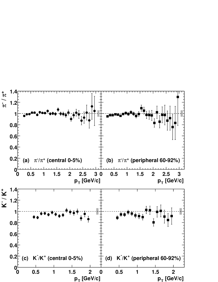
Figure 14 shows the particle ratios of (a) $\pi^{-}/\pi^{+}$ for central 0–5%, (b) $\pi^{-}/\pi^{+}$ for peripheral 60–92%, (c) $K^{-}/K^{+}$ for central 0–5%, and (d) $K^{-}/K^{+}$ for peripheral 60–92%. Similar plots for the $\mbox{$\overline{p}$}/p$ ratios are shown in Figure 15. The error bars represent statistical errors and the shaded boxes on each panel represent the systematic errors. For each of these particle species and centralities, the particle ratios are constant within the experimental errors over the measured $p_{T}$ range. Similar centrality and $p_{T}$ dependences are observed in 130 GeV Au+Au data PPG009 ; STAR_pbarp_130 ; STAR_pbarp_erratum ; STAR_kaon ; STAR_strange ; BRAHMS_pbarp_130 ; PHOBOS_ratio_130 and previously published 200 GeV Au+Au data BRAHMS_ratio_200 ; PHOBOS_ratio_200 .

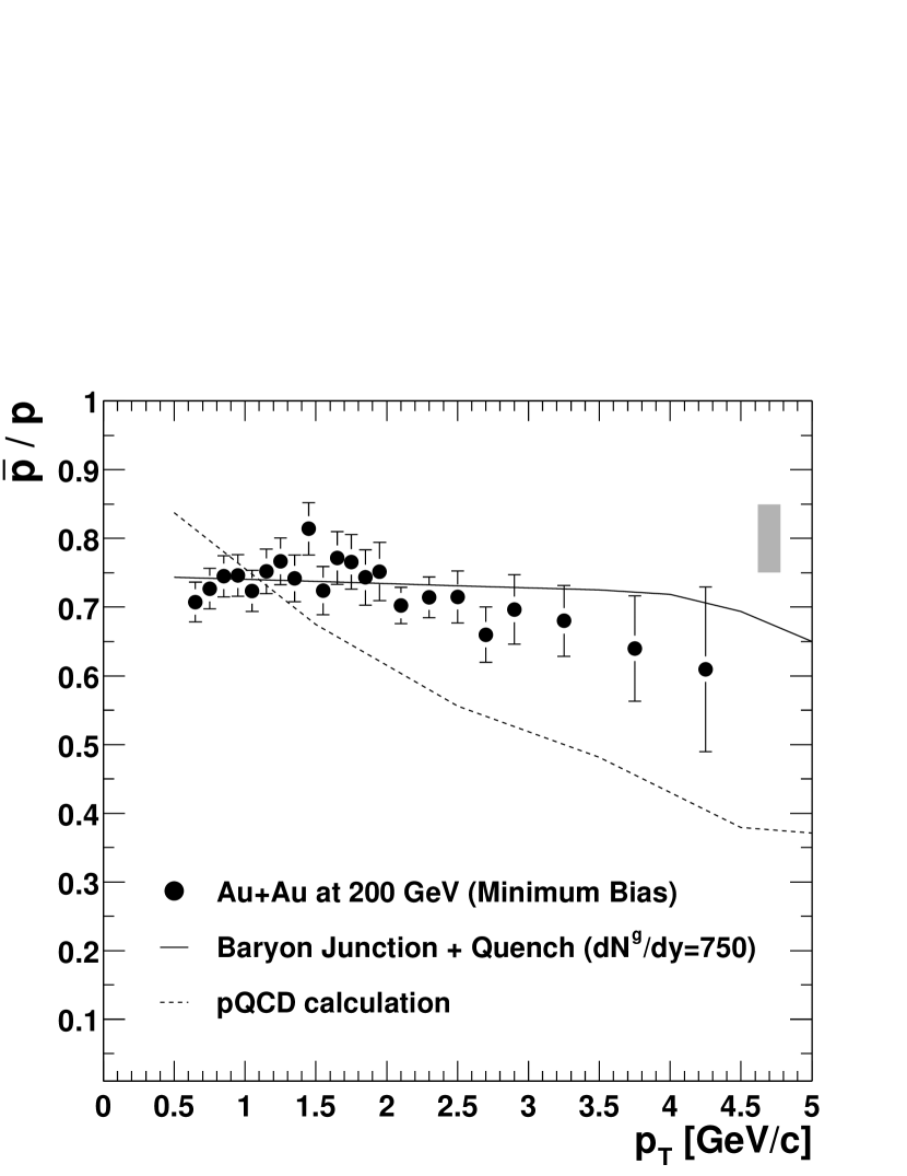
To investigate the $p_{T}$ dependence of the $\mbox{$\overline{p}$}/p$ ratio in detail, it is shown in Figure 16 for minimum bias events with two theoretical calculations: a pQCD calculation (dashed line), and a baryon junction model with jet-quenching bj_pbarp (solid line). The baryon junction calculation agrees well with the measured $\mbox{$\overline{p}$}/p$ ratio over the measured $p_{T}$ range within the experimental uncertainties, while the pQCD calculation does not explain the constant $\mbox{$\overline{p}$}/p$ ratio over the wide $p_{T}$ range. The statistical thermal model (discussed in more detail later in this section) predicted thermal_1 a baryon chemical potential of $\mu_{B}=29$ MeV and a freeze-out temperature of $T_{ch}=177$ MeV for central Au+Au collisions at 200 GeV. From these, the expected $\mbox{$\overline{p}$}/p$ ratio is $e^{-2\mu_{B}/T_{ch}}=0.72$ , which agrees with our data (0.73). The parton recombination model recombination also reproduces the $\mbox{$\overline{p}$}/p$ ratio and its flat $p_{T}$ dependence. The $\mbox{$\overline{p}$}/p$ ratio in this model is 0.72 since the statistical thermal model is used.

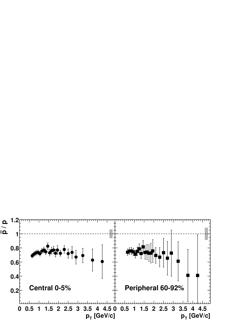
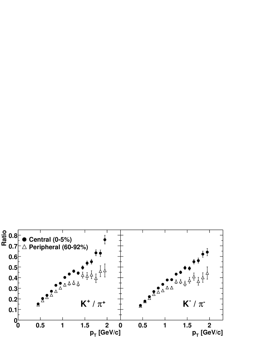
In Figure 17, the $p_{T}$ dependence of the $K/\pi$ ratio is shown for the most central 0–5% and the most peripheral 60–92% centrality bins. The $K^{+}/\pi^{+}$ ( $K^{-}/\pi^{-}$ ) ratios are shown on the left (right). Both ratios increase with $p_{T}$ and the increase is faster in central collisions than in peripheral ones.

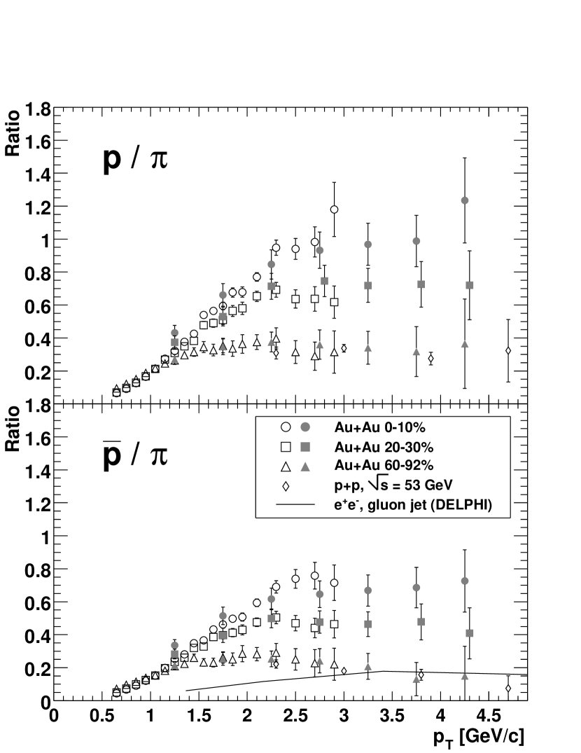
In Figure 18, the $p/\pi$ and $\mbox{$\overline{p}$}/\pi$ ratios are shown as a function of $p_{T}$ for the 0–10%, 20–30% and 60–92% centrality bins. In this figure, the results of $p/\mbox{$\pi^{0}$}$ and $\mbox{$\overline{p}$}/\mbox{$\pi^{0}$}$ PPG014 are presented above 1.5 GeV/ $c$ and overlaid on the results of $p/\pi^{+}$ and $\mbox{$\overline{p}$}/\pi^{-}$ , respectively. The absolutely normalized $p_{T}$ spectra of charged and neutral pions agree within 5–15%. The error bars on the PHENIX data points in the figure show the quadratic sum of the statistical errors and the point-to-point systematic errors. There is an additional normalization uncertainty of 8% for $p/\pi^{+}$ , $\mbox{$\overline{p}$}/\pi^{-}$ and 12% for $p/\mbox{$\pi^{0}$}$ , $\mbox{$\overline{p}$}/\mbox{$\pi^{0}$}$ (the quadratic sum of the systematic errors on $p$ (or $\overline{p}$ ) normalization and $p_{T}$ independent systematic errors from $\pi^{0}$ PPG015 ), which may shift the data up or down for all three centrality bins together, but does not affect their shape. The ratios increase rapidly at low $p_{T}$ , but saturate at different values of $p_{T}$ which increase from peripheral to central collisions. In central collisions, the yields of both protons and anti-protons are comparable to that of pions for $\mbox{$p_{T}$}>2$ GeV/ $c$ . For comparison, the corresponding ratios for $\mbox{$p_{T}$}>$ 2 GeV/ $c$ observed in $p+p$ collisions at lower energies ISR , and in gluon jets produced in $e^{+}+e^{-}$ collisions DELPHI , are also shown. Within the uncertainties those ratios are compatible with the peripheral Au+Au results. In hard-scattering processes described by pQCD, the $p/\pi$ and $\mbox{$\overline{p}$}/\pi$ ratios at high $p_{T}$ are determined by the fragmentation of energetic partons, independent of the initial colliding system, which is seen as agreement between $p+p$ and $e^{+}+e^{-}$ collisions. Thus, the clear increase in the $p/\pi$ ( $\mbox{$\overline{p}$}/\pi$ ) ratios at high $p_{T}$ from $p+p$ and peripheral to the mid-central and to the central Au+Au collisions requires ingredients other than pQCD.

The first observation of the enhancement of protons and anti-protons compared to pions in the intermediate $p_{T}$ region was in the 130 GeV Au+Au data PPG006 . The data inspired several new theoretical interpretations and models. Hydrodynamics calculations Heinz predict that the $\mbox{$\overline{p}$}/\pi$ ratio at high $p_{T}$ exceeds unity for central collisions. The expected $\mbox{$\overline{p}$}/\pi$ ratio in the thermal model at fixed and sufficiently large $p_{T}$ is determined by $2e^{-\mu_{B}/T_{ch}}$ $\approx$ 1.7 using $T_{ch}=177$ MeV and $\mu_{B}=29$ MeV thermal_1 for 200 GeV Au+Au central collisions. Due to the strong radial flow effect at RHIC at relativistic transverse momenta ( $\mbox{$p_{T}$}\gg m$ ), all hadron spectra have a similar shape. The hydrodynamic model thus explains the excess of $\mbox{$\overline{p}$}/\pi$ in central collisions at intermediate $p_{T}$ . However, the hydrodynamic model Cleymans predicts no or very little dependence on the centrality, which clearly disagrees with the present data. This model predicts, within 10%, the same $p_{T}$ dependence of $p/\pi$ ( $\mbox{$\overline{p}$}/\pi$ ) for all centrality bins.

Recently two new models have been proposed to explain the experimental results on the $p_{T}$ dependence of $p/\pi$ and $\mbox{$\overline{p}$}/\pi$ ratios. One model is the parton recombination and fragmentation model recombination and the other model is the baryon junction model bjunctions . Both models explain qualitatively the observed feature of $p/\pi$ enhancement in central collisions, and their centrality dependencies. Furthermore, both theoretical models predict that this baryon enhancement is limited to $\mbox{$p_{T}$}<$ 5 – 6 GeV/ $c$ . This will be discussed in Section IV.5 in detail.

IV.4.2 Particle Ratio versus $N_{part}$

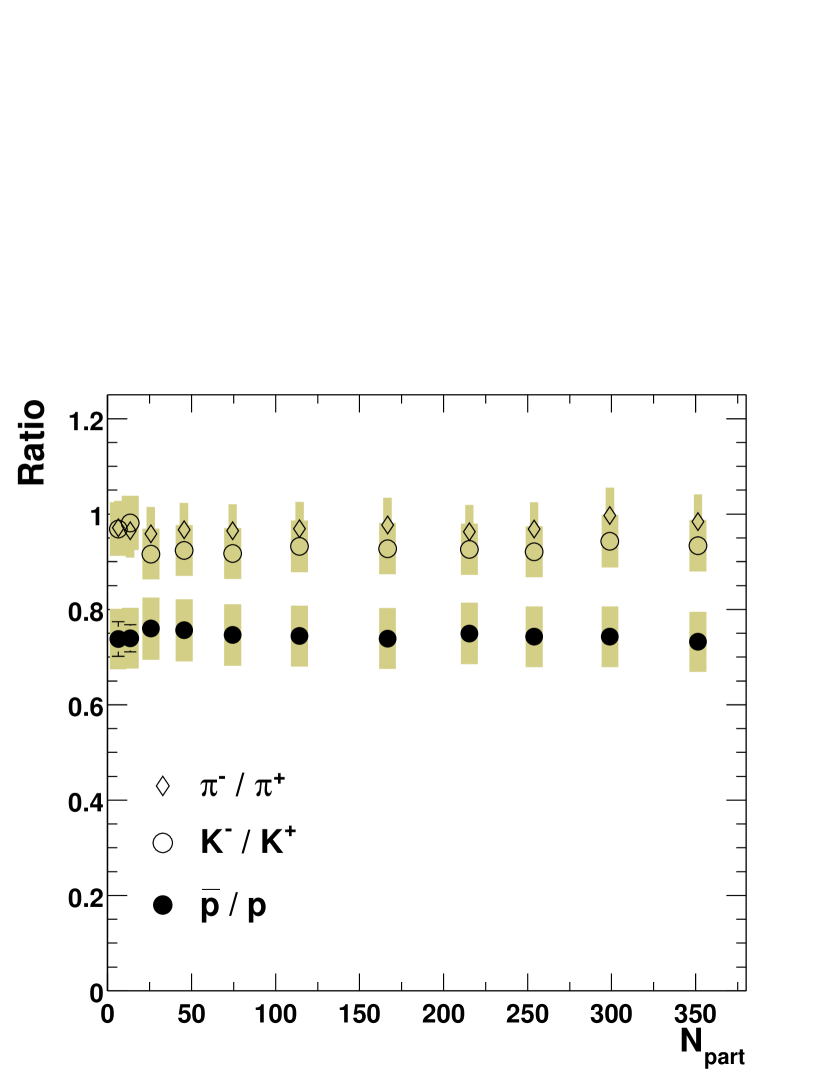
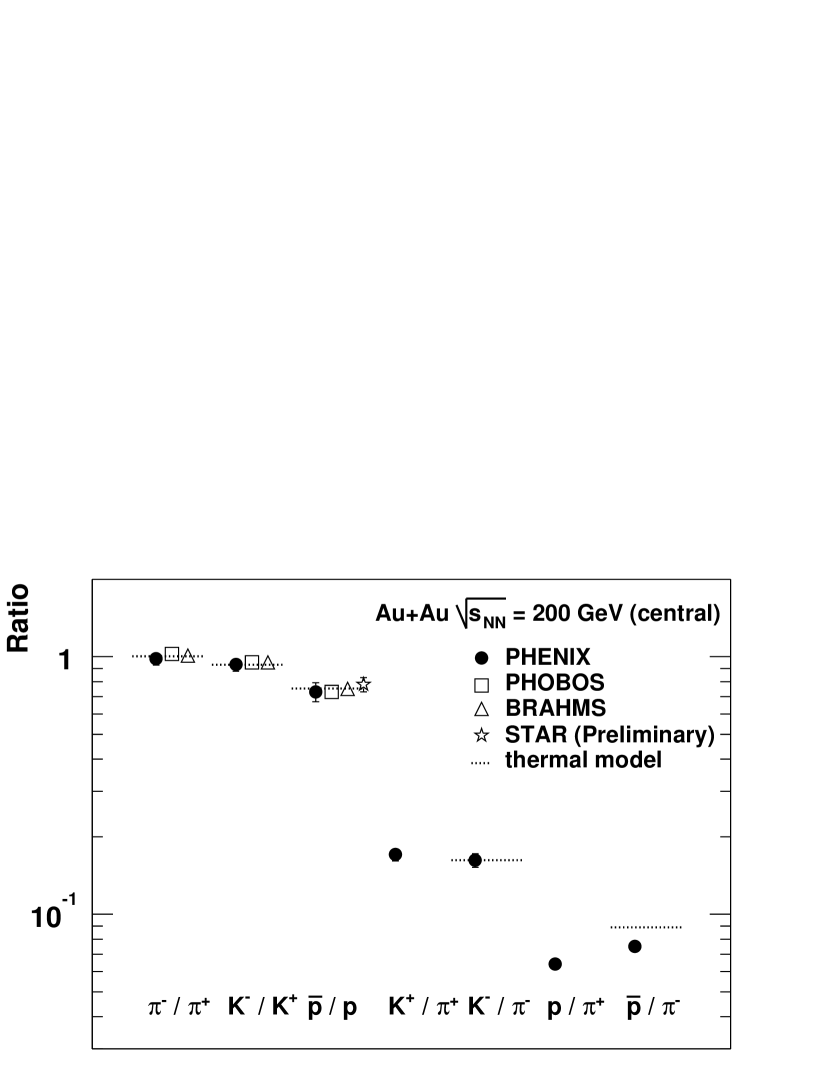
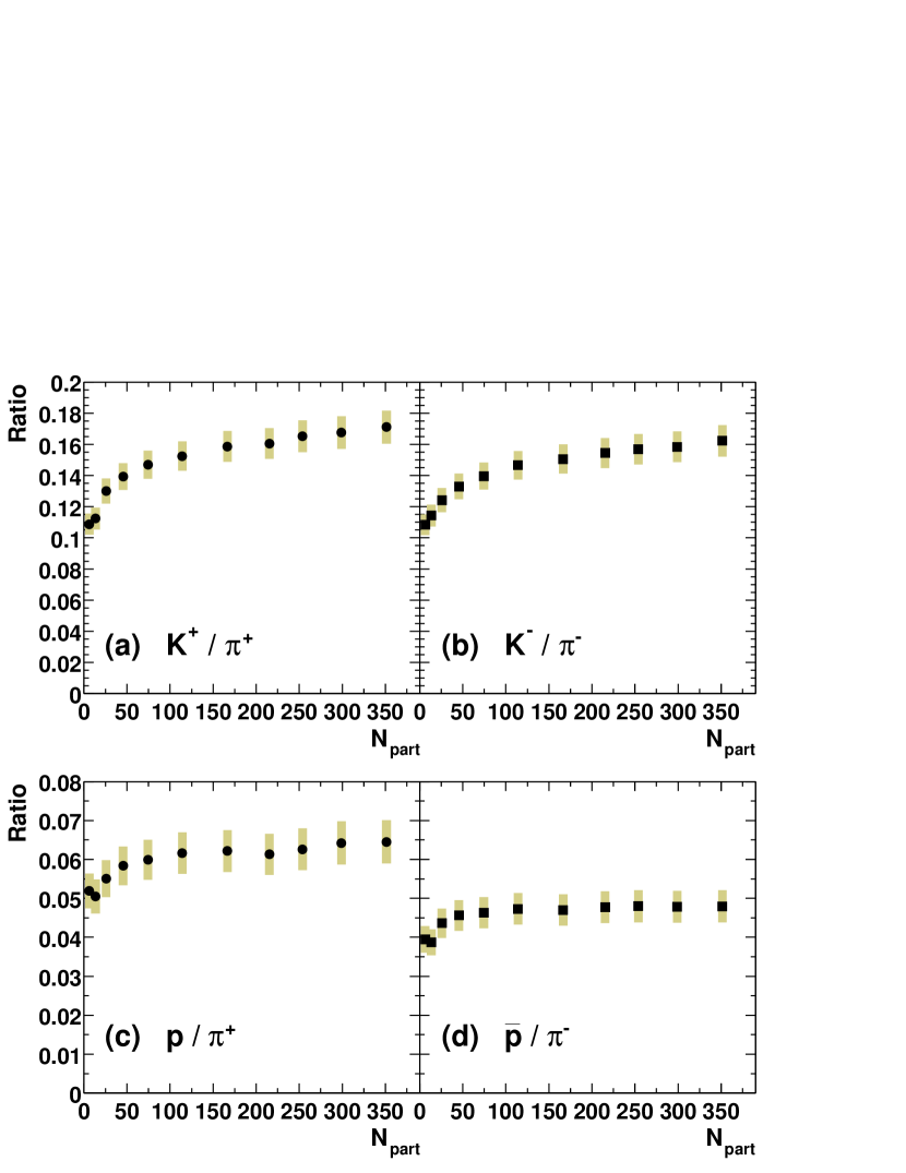
Figure 19 shows the centrality dependence of particle ratios for $\pi^{-}/\pi^{+}$ , $K^{-}/K^{+}$ and $\mbox{$\overline{p}$}/p$ . The ratios presented here are derived from the integrated yields over $p_{T}$ (i.e. $dN/dy$ ). The shaded boxes on each data point indicate the systematic errors. Within uncertainties, the ratios are all independent of $N_{part}$ over the measured range. Figure 20 shows a comparison of the PHENIX particle ratios with those from PHOBOS PHOBOS_ratio_200 , BRAHMS BRAHMS_ratio_200 , and STAR (preliminary) STAR_200_QM02 in Au+Au central collisions at $\sqrt{s_{NN}}$ = 200 GeV at mid-rapidity. The PHENIX anti-particle to particle ratios are consistent with other experimental results within the systematic uncertainties.

Figure 21 shows the centrality dependence of $K/\pi$ and $p/\pi$ ratios. Both $K^{+}/\pi^{+}$ and $K^{-}/\pi^{-}$ ratios increase rapidly for peripheral collisions ( $\mbox{$N_{part}$}<$ 100), and then saturate or rise slowly from the mid-central to the most central collisions. The $p/\pi^{+}$ and $\mbox{$\overline{p}$}/\pi^{-}$ ratios increase for peripheral collisions ( $\mbox{$N_{part}$}<$ 50) and saturate from mid-central to central collisions – similar to the centrality dependence of $K/\pi$ ratio (but possibly flatter).

Within the framework of the statistical thermal model thermal_becattini in a grand canonical ensemble with baryon number, strangeness and charge conservation thermal_1 , particle ratios measured at $\mbox{$\sqrt{s_{NN}}$}=$ 130 GeV at mid-rapidity have been analyzed with the extracted chemical freeze-out temperature $T_{ch}=174\pm 7$ MeV and baryon chemical potential $\mu_{B}=46\pm 5$ MeV. A set of chemical parameters at $\mbox{$\sqrt{s_{NN}}$}=$ 200 GeV in Au+Au were also predicted by using a phenomenological parameterization of the energy dependence of $\mu_{B}$ . The predictions were $\mu_{B}=$ 29 $\pm$ 8 MeV and $T_{ch}=177\pm 7$ MeV at $\mbox{$\sqrt{s_{NN}}$}=$ 200 GeV. The comparison between the PHENIX data at 200 GeV for 0–5% central and the thermal model prediction is shown in Table 9 and Figure 20. There is a good agreement between data and the model. The thermal model calculation was performed by assuming a 50% reconstruction efficiency of all weakly decaying baryons in reference thermal_1 . However, our results have been corrected to remove these contributions. Therefore, Table 9 includes $\mbox{$\overline{p}$}/p$ and $\mbox{$\overline{p}$}/\pi^{-}$ ratios with and without $\Lambda$ ( $\overline{\Lambda}$ ) feed-down corrections to the proton and anti-proton spectra. The ratios without the $\Lambda$ ( $\overline{\Lambda}$ ) feed-down correction are labeled “inclusive”. The small $\mu_{B}$ is qualitatively consistent with our measurement of the number of net protons ( $\approx 5$ ) in central Au+Au collisions at $\mbox{$\sqrt{s_{NN}}$}~{}=~{}200$ GeV at mid-rapidity.

Table 9: Comparison between the data for the 0–5% central collisions and the thermal model prediction at

\sqrt{s_{NN}}

= 200 GeV with

T_{ch}

= 177 MeV and

\mu_{B}

= 29 MeV thermal_1 .

Particles	Ratio $\pm$ stat. $\pm$ sys.	Thermal Model
$\pi^{-}/\pi^{+}$	0.984 $\pm$ 0.004 $\pm$ 0.057	1.004
$K^{-}/K^{+}$	0.933 $\pm$ 0.007 $\pm$ 0.054	0.932
$\mbox{$\overline{p}$}/p$	0.731 $\pm$ 0.011 $\pm$ 0.062
$\mbox{$\overline{p}$}/p$ (inclusive)	0.747 $\pm$ 0.007 $\pm$ 0.046	0.752
$K^{+}/\pi^{+}$	0.171 $\pm$ 0.001 $\pm$ 0.010
$K^{-}/\pi^{-}$	0.162 $\pm$ 0.001 $\pm$ 0.010	0.147
$p/\pi^{+}$	0.064 $\pm$ 0.001 $\pm$ 0.003
$p/\pi^{+}$ (inclusive)	0.099 $\pm$ 0.001 $\pm$ 0.006
$\mbox{$\overline{p}$}/\pi^{-}$	0.047 $\pm$ 0.001 $\pm$ 0.002
$\mbox{$\overline{p}$}/\pi^{-}$ (inclusive)	0.075 $\pm$ 0.001 $\pm$ 0.004	0.089

IV.5 Binary Collision Scaling of $p_{T}$ Spectra

One of the most striking features in Au+Au collisions at RHIC is that $\pi^{0}$ and non-identified hadron yields at $p_{T}>$ 2 GeV/ $c$ in central collisions are suppressed with respect to the number of nucleon-nucleon binary collisions ( $N_{coll}$ ) scaled by $p+p$ and peripheral Au+Au results PPG003 ; PPG013 ; PPG014 . Moreover, the suppression of $\pi^{0}$ is stronger than than that for non-identified charged hadrons PPG003 , and the yields of protons and anti-protons in central collisions are comparable to that of pions around $\mbox{$p_{T}$}=$ 2 GeV/ $c$ PPG006 . The enhancement of the $p/\pi$ ( $\mbox{$\overline{p}$}/\pi$ ) ratio in central collisions at intermediate $p_{T}$ (2.0 – 4.5 GeV/ $c$ ), which was presented in the previous section, is consistent with the above observations. These results show the significant contributions of proton and anti-proton yields to the total particle composition at this intermediate $p_{T}$ region. We present here the $N_{coll}$ scaling behavior for charged pions, kaons, and protons (anti-protons) in order to quantify the particle composition at intermediate $p_{T}$ .

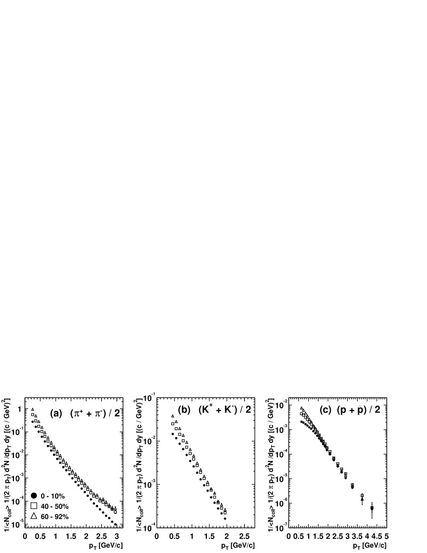
Figure 22 shows the $p_{T}$ spectra scaled by the averaged number of binary collisions, $\langle N_{coll}\rangle$ , for $(\pi^{+}+\pi^{-})/2$ , $(K^{+}+K^{-})/2$ , and $(p+\mbox{$\overline{p}$})/2$ in three centrality bins: central 0–10%, mid-central 40–50% and peripheral 60–92%. For $(p+\mbox{$\overline{p}$})/2$ in the range of $\mbox{$p_{T}$}=$ 1.5 – 4.5 GeV/ $c$ , it is clearly seen that the spectra are on top of each other. This indicates that proton and anti-proton production at high $p_{T}$ scales with the number of binary collisions. On the other hand, at $p_{T}$ below 1.5 GeV/ $c$ , different shapes for different centrality bins are observed, which indicates a strong contribution from radial flow. The scaling behavior of the kaons seems to be similar to protons, but this is not conclusive due to our PID limitations. For pions, the $N_{coll}$ scaled yield in central events is suppressed compared to that for peripheral events at $\mbox{$p_{T}$}>$ 2 GeV/ $c$ , which is consistent with the results in the $\pi^{0}$ spectra PPG003 ; PPG014 .

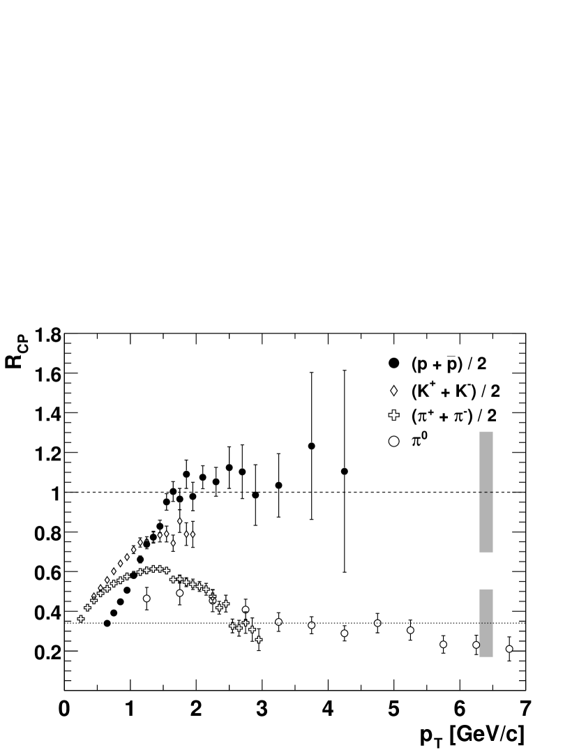
Figure 23 shows the central (0–10%) to peripheral (60–92%) ratio for $N_{coll}$ scaled $p_{T}$ spectra ( $R_{\rm CP}$ : the nuclear modification factor) of $(\mbox{$\overline{p}$}+p)/2$ , kaons, charged pions, and $\pi^{0}$ . In this paper we define $R_{\rm CP}$ as:

R_{\rm CP}=\frac{{\rm Yield^{0-10\%}}/\langle\mbox{$N_{coll}$}^{0-10\%}\rangle}{{\rm Yield^{60-92\%}}/\langle\mbox{$N_{coll}$}^{60-92\%}\rangle}.

(10)

The peripheral 60–92% Au+Au spectrum is used as an approximation of the yields in $p+p$ collisions, based on the experimental fact that the peripheral spectra scale with $N_{coll}$ by using the yields in $p+p$ collisions measured by PHENIX PPG014 ; PPG024 . Thus the meaning of the $R_{\rm CP}$ is expected to be the same as $R_{\rm AA}$ used in our previous publications PPG003 ; PPG013 ; PPG014 . The lines in Figure 23 indicate the expectations of $N_{part}$ (dotted) and $N_{coll}$ (dashed) scaling. The shaded bars at the end of each line represent the systematic error associated with the determination of these quantities for central and peripheral events. The error bars on charged particles are statistical errors only, and those for $\pi^{0}$ are the quadratic sum of the statistical errors and the point-to-point systematic errors. The data show that $(\mbox{$\overline{p}$}+p)/2$ reaches unity for $\mbox{$p_{T}$}\stackrel{{\scriptstyle>}}{{\sim}}$ 1.5 GeV/ $c$ , consistent with $N_{coll}$ scaling. The data for kaons also show the $N_{coll}$ scaling behavior around 1.5 – 2.0 GeV/ $c$ , but the behavior is weaker than for protons. As with neutral pions PPG014 , charged pions are also suppressed at 2 – 3 GeV/ $c$ with respect to peripheral Au+Au collisions.

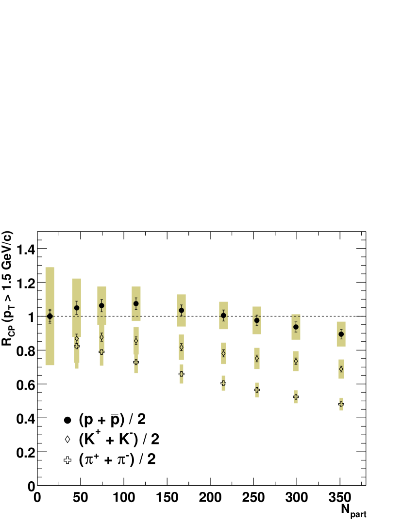
Motivated by the observation that the $(\mbox{$\overline{p}$}+p)/2$ spectra scale with $N_{coll}$ above $\mbox{$p_{T}$}=$ 1.5 GeV/ $c$ , the ratio of the integrated yield between central and peripheral events (scaled by the corresponding $N_{coll}$ ) above $\mbox{$p_{T}$}=$ 1.5 GeV/ $c$ are shown in Figure 24 as a function of $N_{part}$ . The $p_{T}$ ranges for the integration are, 1.5 – 4.5 GeV/ $c$ for $(\mbox{$\overline{p}$}+p)/2$ , 1.5 – 2.0 GeV/ $c$ for kaons, and 1.5 – 3.0 GeV/ $c$ for charged pions. The data points are normalized to the most peripheral data point. The shaded boxes in the figure indicate the systematic errors, which include the normalization errors on the $p_{T}$ spectra, the errors on the detector occupancy corrections, and the uncertainties of the $\langle T_{\rm AuAu}\rangle$ determination for the numerator only. Only at the most peripheral data point, the uncertainty on the denominator $\langle T^{60-92\%}_{\rm AuAu}\rangle$ is also added. The figure shows that $(\mbox{$\overline{p}$}+p)/2$ scales with $N_{coll}$ for all centrality bins, while the data for charged pions show a decrease with $N_{part}$ . The kaon data points are between the charged pions and the $(\mbox{$\overline{p}$}+p)/2$ spectra.

The standard picture of hadron production at high momentum is the fragmentation of energetic partons. While the observed suppression of the $\pi^{0}$ yield at high $p_{T}$ in central collisions may be attributed to the energy loss of partons during their propagation through the hot and dense matter created in the collisions, i.e. jet quenching quench_effect ; quenching_theory , it is a theoretical challenge to explain the absence of suppression for baryons up to 4.5 GeV/ $c$ for all centralities along with the enhancement of the $p/\pi$ ratio at $\mbox{$p_{T}$}=$ 2 – 4 GeV/ $c$ for central collisions.

It has been recently proposed that such observations can be explained by the dominance of parton recombination at intermediate $p_{T}$ , rather than by fragmentation recombination . The competition between recombination and fragmentation of partons may explain the observed features. The model predicts that the effect is limited to $\mbox{$p_{T}$}<5$ GeV/ $c$ , beyond which fragmentation becomes the dominant production mechanism for all particle species.

Another possible explanation is the baryon junction model bjunctions . It invokes a topological gluon configuration with jet quenching. With pion production above 2 GeV/ $c$ suppressed by jet quenching, gluon junctions produce copious baryons at intermediate $p_{T}$ , thus lead to the enhancement of baryons in this $p_{T}$ region. The model reproduces the baryon-to-meson ratio and its centrality dependence qualitatively ptopi_bjunctions .

Both theoretical models predict that baryon enhancement is limited to $\mbox{$p_{T}$}<$ 5 – 6 GeV/ $c$ , which is unfortunately beyond our current PID capability. However, it is possible to test the two predictions indirectly by using the non-identified charged hadrons to neutral pion ratio ( $h/\mbox{$\pi^{0}$}$ ) as a measure of the baryon content at high $p_{T}$ , as published in PPG015 . The results support the limited behavior of baryon enhancement up to 5 GeV/ $c$ in $p_{T}$ . Similar trends are observed in $\Lambda$ , $K^{0}_{S}$ and $K^{\pm}$ measurements by the STAR collaboration STAR_k0 .

On the other hand, it is also possible that nuclear effects, such as the “Cronin effect” cronin1975 ; antreasyan1979 , attributed to initial state multiple scattering ( $p_{T}$ -broadening) pt_broadening , contribute to the observed species dependence. At center-of-mass energies up to $\sqrt{s}=38.8$ GeV, a nuclear enhancement beyond $N_{coll}$ scaling has been observed for $\pi,K,p$ and their anti-particles in $p+A$ collisions. The effect is stronger for protons and anti-protons than for pions which leads to an enhancement of the $p/\pi$ and $\mbox{$\overline{p}$}/\pi$ ratios compared to $p+p$ collisions. In proton-tungsten reactions, the increase is a factor of $\sim 2$ in the range 3 $<\mbox{$p_{T}$}<$ 6 GeV. For pions, theoretical calculations at RHIC energies Cronin_RHIC predict a reduced strength of the Cronin effect compared to lower energies, although no prediction exists for protons. New data from d+Au collisions at $\sqrt{s_{NN}}$ = 200 GeV will help to clarify this issue.

V SUMMARY AND CONCLUSION

In summary, we present the centrality dependence of identified charged hadron spectra and yields for $\pi^{\pm}$ , $K^{\pm}$ , $p$ and $\overline{p}$ in Au+Au collisions at $\sqrt{s_{NN}}$ = 200 GeV at mid-rapidity. In central events, the low $p_{T}$ region ( $\leq$ 2.0 GeV/ $c$ ) of the $p_{T}$ spectra show a clear particle mass dependence in their shapes, namely, $p$ and $\overline{p}$ spectra have a shoulder-arm shape while the pion spectra have a concave shape. The spectra can be well fit with an exponential function in $m_{T}$ at the region below 1.0 GeV/ $c^{2}$ in $\mbox{$m_{T}$}-m_{0}$ . The resulting inverse slope parameters show clear particle mass and centrality dependences, that increase with particle mass and centrality. These observations are consistent with the hydrodynamic radial flow picture. Moreover, at around $\mbox{$p_{T}$}=$ 2.0 GeV/ $c$ in central events, the $p$ and $\overline{p}$ yields are comparable to the pion yields. Here, baryons comprise a significant fraction of the hadron yield in this intermediate $p_{T}$ range. The $\langle p_{T}\rangle$ and $dN/dy$ per participant pair increase from peripheral to mid-central collisions and saturate for the most central collisions for all particle species. The net proton number in Au+Au central collisions at $\sqrt{s_{NN}}$ = 200 GeV is $\sim$ 5 at mid-rapidity.

The particle ratios of $\pi^{-}/\pi^{+}$ , $K^{-}/K^{+}$ , $p/\mbox{$\overline{p}$}$ , $K/\pi$ , $p/\pi$ and $\mbox{$\overline{p}$}/\pi$ as a function of $p_{T}$ and centrality have been measured. Particle ratios in central Au+Au collisions are well reproduced by the statistical thermal model with a baryon chemical potential of $\mu_{B}$ = 29 MeV and a chemical freeze-out temperature of $T_{ch}$ = 177 MeV. Regardless of the particle species and centrality, it is found that ratios for equal mass particles are constant as a function of $p_{T}$ , within the systematic uncertainties in the measured $p_{T}$ range. On the other hand, both $K/\pi$ and $p/\pi$ ( $\mbox{$\overline{p}$}/\pi$ ) ratios increase as a function of $p_{T}$ . This increase with $p_{T}$ is stronger for central than for peripheral events. The $p/\pi$ and $\mbox{$\overline{p}$}/\pi$ ratios in central events both increase with $p_{T}$ up to 3 GeV/ $c$ and approach unity at $\mbox{$p_{T}$}\approx$ 2 GeV/ $c$ . However, in peripheral collisions these ratios saturate at the value of 0.3 – 0.4 around $\mbox{$p_{T}$}=$ 1.5 GeV/ $c$ . The observed centrality dependence of $p/\pi$ and $\mbox{$\overline{p}$}/p$ ratios in intermediate $p_{T}$ region is not explained by the hydrodynamic model alone, but both the parton recombination model and the baryon junction model qualitatively agree with data.

The scaling behavior of identified charged hadrons is compared with results for neutral pions. In the $N_{coll}$ scaled $p_{T}$ spectra for $(p+\mbox{$\overline{p}$})/2$ , the spectra scale with $N_{coll}$ from $\mbox{$p_{T}$}=$ 1.5 – 4.5 GeV/ $c$ . The central-to-peripheral ratio, $R_{CP}$ , approaches unity for $(\mbox{$\overline{p}$}+p)/2$ from $\mbox{$p_{T}$}=$ 1.5 up to 4.5 GeV/ $c$ . Meanwhile, charged and neutral pions are suppressed. The ratio of integrated $R_{CP}$ from $\mbox{$p_{T}$}=$ 1.5 to 4.5 GeV/ $c$ exhibits an $N_{coll}$ scaling behavior for all centrality bins in the $(\mbox{$\overline{p}$}+p)/2$ data, which is in contrast to the stronger pion suppression, that increases with centrality.

Appendix A Table of Invariant Yields

The invariant yields for $\pi^{\pm}$ , $K^{\pm}$ , $p$ and $\overline{p}$ in Au+Au collisions at $\sqrt{s_{NN}}$ = 200 GeV at mid-rapidity are tabulated in Tables 10 – 29. The data presented here are for the the minimum bias events and each centrality bin (0–5%, 5–10%, 10–15%, 15–20%, 20–30%, …, 70–80%, 80–92%, and 60–92%). Errors are statistical only.

Acknowledgements.

We thank the staff of the Collider-Accelerator and Physics Departments at Brookhaven National Laboratory and the staff of the other PHENIX participating institutions for their vital contributions. We acknowledge support from the Department of Energy, Office of Science, Nuclear Physics Division, the National Science Foundation, Abilene Christian University Research Council, Research Foundation of SUNY, and Dean of the College of Arts and Sciences, Vanderbilt University (U.S.A), Ministry of Education, Culture, Sports, Science, and Technology and the Japan Society for the Promotion of Science (Japan), Conselho Nacional de Desenvolvimento Científico e Tecnológico and Fundação de Amparo à Pesquisa do Estado de São Paulo (Brazil), Natural Science Foundation of China (People’s Republic of China), Centre National de la Recherche Scientifique, Commissariat à l’Énergie Atomique, Institut National de Physique Nucléaire et de Physique des Particules, and Institut National de Physique Nucléaire et de Physique des Particules, (France), Bundesministerium fuer Bildung und Forschung, Deutscher Akademischer Austausch Dienst, and Alexander von Humboldt Stiftung (Germany), Hungarian National Science Fund, OTKA (Hungary), Department of Atomic Energy and Department of Science and Technology (India), Israel Science Foundation (Israel), Korea Research Foundation and Center for High Energy Physics (Korea), Russian Ministry of Industry, Science and Tekhnologies, Russian Academy of Science, Russian Ministry of Atomic Energy (Russia), VR and the Wallenberg Foundation (Sweden), the U.S. Civilian Research and Development Foundation for the Independent States of the Former Soviet Union, the US-Hungarian NSF-OTKA-MTA, the US-Israel Binational Science Foundation, and the 5th European Union TMR Marie-Curie Programme.

References

(1) See E. Laermann and O. Philipsen, hep-ph/0303042 (to appear in Ann. Rev. Nuc. Part. Sci.), for a recent review.
(2) J. D. Bjorken, Phys. Rev. D 27, 140 (1983).
(3) PHENIX Collaboration, K. Adcox et al., Phys. Rev. Lett. 87, 052301 (2001).
(4) W. Broniowski and W. Florkowski, Phys. Rev. Lett. 87, 272302 (2001); W. Broniowski and W. Florkowski, Phys. Rev. C 65, 064905 (2002).
(5) D. Teaney, J. Lauret, and E. V. Shuryak, nucl-th/0110037; D. Teaney, J. Lauret, and E. V. Shuryak, Phys. Rev. Lett. 86, 4783 (2001).
(6) PHENIX Collaboration, K. Adcox et al., Phys. Rev. Lett. 88, 242301 (2002).
(7) STAR Collaboration, C. Adler et al., Phys. Rev. Lett. 87, 262302 (2001).
(8) PHENIX Collaboration, K. Adcox et al., submitted to Phys. Rev. C , nucl-ex/0307010.
(9) F. Becattini et al., Phys. Rev. C 64, 024901 (2001).
(10) P.Braun-Munzinger, D.Magestro, K.Redlich, J.Stachel, Phys. Lett. B 518, 41 (2001).
(11) W. Florkowski, W. Broniowski, and M. Michalec, Acta Phys. Polon. B 33, 761 (2002).
(12) PHENIX Collaboration, K. Adcox et al., Phys. Rev. Lett. 88, 022301 (2002).
(13) PHENIX Collaboration, K. Adcox et al., Phys. Lett. B 561, 82 (2003)
(14) PHENIX Collaboration, S. S. Adler et al., submitted to Phys. Rev. Lett. , nucl-ex/0304022.
(15) X. N. Wang and M. Gyulassy, Phys. Rev. Lett. 68, 1480 (1992); X. N. Wang, Phys. Rev. C 58, 2321 (1998).
(16) M. Gyulassy and M. Plümer, Phys. Lett. B 243, 432 (1990); R. Baier et al., Phys. Lett. B 345, 277 (1995).
(17) PHENIX Collaboration, K. Adcox et al., Nucl. Instrum. Methods A 499, 469 (2003)
(18) PHENIX Collaboration, M. Aizawa et al., Nucl. Instrum. Methods A 499, 508 (2003)
(19) PHENIX Collaboration, L. Aphecetche et al., Nucl. Instrum. Methods A 499, 521 (2003)
(20) PHENIX Collaboration, M. Allen et al., Nucl. Instrum. Methods A 499, 549 (2003)
(21) PHENIX Collaboration, C. Adler et al., Nucl. Instrum. Methods A 470, 488 (2001)
(22) PHENIX Collaboration, K. Adcox et al., Nucl. Instrum. Methods A 499, 489 (2003)
(23) PHENIX Collaboration, S. S. Adler et al., submitted to Phys. Rev. Lett. , nucl-ex/0305036.
(24) PHENIX Collaboration, S. S. Adler et al., submitted to Phys. Rev. Lett. , hep-ex/0304038.
(25) J. T. Mitchell et al., Nucl. Instrum. Methods A 482, 491 (2002).
(26) GEANT 3.21, CERN program library.
(27) X. N. Wang and M. Gyulassy, Phys. Rev. D 44, 3501 (1991), version 1.35.
(28) PHENIX Collaboration, K. Adcox et al., Phys. Rev. Lett. 89, 092302 (2002).
(29) P. F. Kolb and R. Rapp, Phys. Rev. C 67, 044903 (2003).
(30) E. Schnedermann, J. Sollfrank, and U. Heinz, Phys. Rev. C 48, 2462 (1993)
(31) P. Kolb et al., Nucl. Phys. A 696, 197 (2001); P. Huovinen et al., Phys. Lett. B 503, 58 (2001).
(32) U. Heinz, P. Kolb, Nucl. Phys. A 702, 269 (2002).
(33) E. Schnedermann, J. Sollfrank, and U. Heinz, Phys. Rev. C 48, 2462 (1994); T. Csörgő and B. Lörstad, Phys. Rev. C 54, 1390 (1996).
(34) T. Csörgő, S. V. Akkelin, Y. Hama, B. Lukács and Y.M. Sinyukov, Phys. Rev. C 67, 034904 (2003).
(35) J. Schaffner-Bielich, D. Kharzeev, L. McLerran and R. Venugopalan, Nucl. Phys. A 705, 494 (2002).
(36) P. Christiansen for the BRAHMS Collaboration, nucl-ex/0212002.
(37) STAR Collaboration, C. Adler et al., Phys. Rev. Lett. 86, 4778 (2001).
(38) STAR Collaboration, J. Adams et al., to appear in Phys. Rev. Lett. .
(39) STAR Collaboration, C. Adler et al., to appear in Phys. Lett. B , nucl-ex/0206008.
(40) STAR Collaboration, C. Adler et al., to appear in Phys. Lett. B .
(41) BRAHMS Collaboration, I. G. Bearden et al., Phys. Rev. Lett. 87, 112305 (2001).
(42) PHOBOS Collaboration, B. B. Back et al., Phys. Rev. Lett. 87, 102301 (2001).
(43) BRAHMS Collaboration, I. G. Bearden et al., Phys. Rev. Lett. 90, 102301 (2003).
(44) PHOBOS Collaboration, B. B. Back et al., Phys. Rev. C 67, 021901(R) (2003).
(45) R. C. Hwa and C. B. Yang, Phys. Rev. C 67, 034902 (2003); R. J. Fries, B. Müller, C. Nonaka and S. A. Bass, nucl-th/0301087; V. Greco, C. M. Ko and P. Lévai, nucl-th/0301093.
(46) I. Vitev and M. Gyulassy, Nucl. Phys. A 715, 779c (2003).
(47) B. Alper et al., Nucl. Phys. B 100, 237 (1975).
(48) DELPHI Collaboration, P. Abreu et al. Eur. Phys. J. C17, 207 (2000).
(49) B. Kämpfer, J. Cleymans, K. Gallmeister, S. M. Wheaton, hep-ph/0204227.
(50) G.C. Rossi and G. Veneziano, Nucl. Phys. B 123, 507 (1977); D. Kharzeev, Phys. Lett. B 378, 238 (1996); S.E. Vance, M. Gyulassy, X.-N. Wang, Phys. Lett. B 443, 45 (1998).
(51) G. Van Buren, Nucl. Phys. A 715, 129c (2003).
(52) I. Vitev and M. Gyulassy, Phys. Rev. C 65, 041902 (2002); I. Vitev, M. Gyulassy, P. Lévai, hep-ph/0109198.
(53) STAR Collaboration, J. Adams et al., submitted to Phys. Rev. Lett. , nucl-ex/0306007.
(54) J. Cronin et al., Phys. Rev. D 11, 3105 (1975).
(55) D. Antreasyan et al., Phys. Rev. D 19, 764 (1979).
(56) M. Lev, B. Petersson, Z. Phys. C 21, 155 (83).
(57) B. Z. Kopeliovich, J. Nemchik, A. Schafer, A. V. Tarasov Phys. Rev. Lett. 88, 232303 (2002).

Table 10: Invariant yields for

\pi^{+}

at mid-rapidity in the minimum bias, 0–5%, 5–10%, and 10–15% centrality bins, normalized to one unit rapidity. Errors are statistical only.

$p_{T}$ [GeV/ $c$ ]	Minimum bias	0–5%	5–10%	10–15%
0.25	1.07e+02 $\pm$ 8.8e-01	3.29e+02 $\pm$ 2.7e+00	2.76e+02 $\pm$ 2.3e+00	2.39e+02 $\pm$ 2.0e+00
0.35	6.06e+01 $\pm$ 5.0e-01	1.97e+02 $\pm$ 1.6e+00	1.64e+02 $\pm$ 1.4e+00	1.39e+02 $\pm$ 1.2e+00
0.45	3.63e+01 $\pm$ 3.1e-01	1.20e+02 $\pm$ 1.1e+00	9.93e+01 $\pm$ 8.7e-01	8.41e+01 $\pm$ 7.4e-01
0.55	2.18e+01 $\pm$ 2.0e-01	7.26e+01 $\pm$ 6.7e-01	6.02e+01 $\pm$ 5.6e-01	5.08e+01 $\pm$ 4.7e-01
0.65	1.34e+01 $\pm$ 1.3e-01	4.49e+01 $\pm$ 4.5e-01	3.74e+01 $\pm$ 3.8e-01	3.16e+01 $\pm$ 3.2e-01
0.75	8.71e+00 $\pm$ 9.5e-02	2.93e+01 $\pm$ 3.3e-01	2.43e+01 $\pm$ 2.7e-01	2.05e+01 $\pm$ 2.3e-01
0.85	5.41e+00 $\pm$ 6.3e-02	1.82e+01 $\pm$ 2.2e-01	1.53e+01 $\pm$ 1.8e-01	1.29e+01 $\pm$ 1.6e-01
0.95	3.59e+00 $\pm$ 4.5e-02	1.21e+01 $\pm$ 1.6e-01	1.01e+01 $\pm$ 1.3e-01	8.56e+00 $\pm$ 1.1e-01
1.05	2.35e+00 $\pm$ 3.1e-02	7.96e+00 $\pm$ 1.1e-01	6.56e+00 $\pm$ 9.3e-02	5.56e+00 $\pm$ 8.0e-02
1.15	1.58e+00 $\pm$ 2.2e-02	5.32e+00 $\pm$ 8.0e-02	4.47e+00 $\pm$ 6.8e-02	3.72e+00 $\pm$ 5.7e-02
1.25	1.05e+00 $\pm$ 1.5e-02	3.55e+00 $\pm$ 5.7e-02	2.99e+00 $\pm$ 4.9e-02	2.51e+00 $\pm$ 4.2e-02
1.35	7.59e-01 $\pm$ 1.2e-02	2.55e+00 $\pm$ 4.5e-02	2.15e+00 $\pm$ 3.9e-02	1.81e+00 $\pm$ 3.3e-02
1.45	5.16e-01 $\pm$ 8.3e-03	1.72e+00 $\pm$ 3.3e-02	1.45e+00 $\pm$ 2.8e-02	1.23e+00 $\pm$ 2.5e-02
1.55	3.37e-01 $\pm$ 5.6e-03	1.13e+00 $\pm$ 2.3e-02	9.36e-01 $\pm$ 2.0e-02	7.93e-01 $\pm$ 1.7e-02
1.65	2.44e-01 $\pm$ 4.2e-03	8.05e-01 $\pm$ 1.8e-02	6.68e-01 $\pm$ 1.6e-02	5.78e-01 $\pm$ 1.4e-02
1.75	1.77e-01 $\pm$ 3.3e-03	5.70e-01 $\pm$ 1.4e-02	4.84e-01 $\pm$ 1.3e-02	4.19e-01 $\pm$ 1.1e-02
1.85	1.27e-01 $\pm$ 2.4e-03	4.18e-01 $\pm$ 1.2e-02	3.42e-01 $\pm$ 1.0e-02	2.99e-01 $\pm$ 9.1e-03
1.95	9.01e-02 $\pm$ 1.9e-03	2.80e-01 $\pm$ 9.0e-03	2.50e-01 $\pm$ 8.3e-03	2.07e-01 $\pm$ 7.3e-03
2.05	6.68e-02 $\pm$ 1.2e-03	2.09e-01 $\pm$ 6.1e-03	1.82e-01 $\pm$ 5.6e-03	1.56e-01 $\pm$ 5.0e-03
2.15	4.71e-02 $\pm$ 8.9e-04	1.36e-01 $\pm$ 4.8e-03	1.27e-01 $\pm$ 4.6e-03	1.05e-01 $\pm$ 4.1e-03
2.25	3.27e-02 $\pm$ 6.8e-04	9.10e-02 $\pm$ 3.8e-03	8.06e-02 $\pm$ 3.5e-03	8.05e-02 $\pm$ 3.5e-03
2.35	2.60e-02 $\pm$ 6.2e-04	7.20e-02 $\pm$ 3.6e-03	6.28e-02 $\pm$ 3.3e-03	5.78e-02 $\pm$ 3.1e-03
2.45	1.94e-02 $\pm$ 5.3e-04	5.40e-02 $\pm$ 3.2e-03	4.57e-02 $\pm$ 2.9e-03	4.06e-02 $\pm$ 2.7e-03
2.55	1.49e-02 $\pm$ 4.7e-04	3.78e-02 $\pm$ 2.8e-03	3.59e-02 $\pm$ 2.7e-03	3.18e-02 $\pm$ 2.5e-03
2.65	1.13e-02 $\pm$ 4.2e-04	2.65e-02 $\pm$ 2.5e-03	2.50e-02 $\pm$ 2.4e-03	2.44e-02 $\pm$ 2.3e-03
2.75	9.30e-03 $\pm$ 4.0e-04	2.27e-02 $\pm$ 2.5e-03	2.19e-02 $\pm$ 2.4e-03	1.83e-02 $\pm$ 2.1e-03
2.85	6.20e-03 $\pm$ 3.2e-04	1.28e-02 $\pm$ 1.9e-03	1.21e-02 $\pm$ 1.8e-03	1.30e-02 $\pm$ 1.8e-03
2.95	5.17e-03 $\pm$ 3.1e-04	1.03e-02 $\pm$ 1.8e-03	1.08e-02 $\pm$ 1.8e-03	1.04e-02 $\pm$ 1.8e-03

Table 11: Invariant yields for

\pi^{+}

at mid-rapidity in 15–20%, 20–30%, 30–40%, and 40-50% centrality bins, normalized to one unit rapidity. Errors are statistical only.

$p_{T}$ [GeV/ $c$ ]	15–20%	20–30%	30–40%	40–50%
0.25	2.04e+02 $\pm$ 1.7e+00	1.57e+02 $\pm$ 1.3e+00	1.07e+02 $\pm$ 8.9e-01	6.84e+01 $\pm$ 5.7e-01
0.35	1.18e+02 $\pm$ 9.9e-01	8.82e+01 $\pm$ 7.4e-01	5.86e+01 $\pm$ 4.9e-01	3.67e+01 $\pm$ 3.1e-01
0.45	7.09e+01 $\pm$ 6.2e-01	5.27e+01 $\pm$ 4.6e-01	3.46e+01 $\pm$ 3.0e-01	2.15e+01 $\pm$ 1.9e-01
0.55	4.28e+01 $\pm$ 4.0e-01	3.17e+01 $\pm$ 2.9e-01	2.06e+01 $\pm$ 1.9e-01	1.26e+01 $\pm$ 1.2e-01
0.65	2.65e+01 $\pm$ 2.7e-01	1.95e+01 $\pm$ 2.0e-01	1.26e+01 $\pm$ 1.3e-01	7.66e+00 $\pm$ 8.0e-02
0.75	1.73e+01 $\pm$ 2.0e-01	1.27e+01 $\pm$ 1.4e-01	8.29e+00 $\pm$ 9.4e-02	4.99e+00 $\pm$ 5.8e-02
0.85	1.07e+01 $\pm$ 1.3e-01	7.94e+00 $\pm$ 9.5e-02	5.10e+00 $\pm$ 6.3e-02	3.04e+00 $\pm$ 3.9e-02
0.95	7.12e+00 $\pm$ 9.6e-02	5.31e+00 $\pm$ 7.0e-02	3.38e+00 $\pm$ 4.6e-02	2.02e+00 $\pm$ 2.9e-02
1.05	4.77e+00 $\pm$ 6.9e-02	3.49e+00 $\pm$ 4.9e-02	2.22e+00 $\pm$ 3.2e-02	1.30e+00 $\pm$ 2.0e-02
1.15	3.16e+00 $\pm$ 5.0e-02	2.34e+00 $\pm$ 3.5e-02	1.50e+00 $\pm$ 2.4e-02	8.78e-01 $\pm$ 1.5e-02
1.25	2.10e+00 $\pm$ 3.6e-02	1.56e+00 $\pm$ 2.5e-02	9.99e-01 $\pm$ 1.7e-02	5.98e-01 $\pm$ 1.1e-02
1.35	1.52e+00 $\pm$ 2.9e-02	1.12e+00 $\pm$ 2.0e-02	7.17e-01 $\pm$ 1.4e-02	4.26e-01 $\pm$ 9.0e-03
1.45	1.05e+00 $\pm$ 2.2e-02	7.57e-01 $\pm$ 1.5e-02	4.98e-01 $\pm$ 1.0e-02	2.91e-01 $\pm$ 6.9e-03
1.55	6.78e-01 $\pm$ 1.5e-02	5.07e-01 $\pm$ 1.0e-02	3.24e-01 $\pm$ 7.4e-03	1.97e-01 $\pm$ 5.2e-03
1.65	4.93e-01 $\pm$ 1.2e-02	3.67e-01 $\pm$ 8.3e-03	2.31e-01 $\pm$ 5.9e-03	1.42e-01 $\pm$ 4.2e-03
1.75	3.60e-01 $\pm$ 1.0e-02	2.67e-01 $\pm$ 6.7e-03	1.69e-01 $\pm$ 4.9e-03	1.03e-01 $\pm$ 3.5e-03
1.85	2.56e-01 $\pm$ 8.2e-03	1.92e-01 $\pm$ 5.3e-03	1.22e-01 $\pm$ 3.9e-03	7.29e-02 $\pm$ 2.8e-03
1.95	1.78e-01 $\pm$ 6.6e-03	1.38e-01 $\pm$ 4.3e-03	8.80e-02 $\pm$ 3.3e-03	5.80e-02 $\pm$ 2.5e-03
2.05	1.35e-01 $\pm$ 4.6e-03	1.00e-01 $\pm$ 2.9e-03	6.67e-02 $\pm$ 2.3e-03	4.13e-02 $\pm$ 1.7e-03
2.15	1.02e-01 $\pm$ 4.0e-03	7.41e-02 $\pm$ 2.4e-03	4.90e-02 $\pm$ 1.9e-03	2.92e-02 $\pm$ 1.4e-03
2.25	6.65e-02 $\pm$ 3.1e-03	5.16e-02 $\pm$ 2.0e-03	3.58e-02 $\pm$ 1.6e-03	2.09e-02 $\pm$ 1.2e-03
2.35	5.43e-02 $\pm$ 3.0e-03	4.12e-02 $\pm$ 1.9e-03	2.84e-02 $\pm$ 1.5e-03	1.87e-02 $\pm$ 1.2e-03
2.45	3.97e-02 $\pm$ 2.6e-03	3.28e-02 $\pm$ 1.7e-03	2.27e-02 $\pm$ 1.4e-03	1.21e-02 $\pm$ 9.8e-04
2.55	2.88e-02 $\pm$ 2.4e-03	2.41e-02 $\pm$ 1.5e-03	1.70e-02 $\pm$ 1.3e-03	1.11e-02 $\pm$ 1.0e-03
2.65	2.21e-02 $\pm$ 2.2e-03	1.85e-02 $\pm$ 1.4e-03	1.40e-02 $\pm$ 1.2e-03	8.92e-03 $\pm$ 9.5e-04
2.75	1.58e-02 $\pm$ 2.0e-03	1.55e-02 $\pm$ 1.4e-03	1.20e-02 $\pm$ 1.2e-03	7.80e-03 $\pm$ 9.5e-04
2.85	1.37e-02 $\pm$ 1.9e-03	1.03e-02 $\pm$ 1.1e-03	7.69e-03 $\pm$ 9.7e-04	5.80e-03 $\pm$ 8.3e-04
2.95	1.08e-02 $\pm$ 1.8e-03	9.32e-03 $\pm$ 1.2e-03	6.39e-03 $\pm$ 9.6e-04	4.49e-03 $\pm$ 7.9e-04

Table 12: Invariant yields for

\pi^{+}

at mid-rapidity in 50–60%, 60–70%, 70–80%, and 80-92% centrality bins, normalized to one unit rapidity. Errors are statistical only.

$p_{T}$ [GeV/ $c$ ]	50–60%	60–70%	70–80%	80–92%
0.25	4.10e+01 $\pm$ 3.4e-01	2.19e+01 $\pm$ 1.9e-01	1.03e+01 $\pm$ 9.2e-02	5.20e+00 $\pm$ 5.0e-02
0.35	2.17e+01 $\pm$ 1.9e-01	1.13e+01 $\pm$ 1.0e-01	5.27e+00 $\pm$ 5.0e-02	2.75e+00 $\pm$ 2.8e-02
0.45	1.24e+01 $\pm$ 1.1e-01	6.37e+00 $\pm$ 6.0e-02	2.95e+00 $\pm$ 3.1e-02	1.49e+00 $\pm$ 1.8e-02
0.55	7.20e+00 $\pm$ 7.0e-02	3.65e+00 $\pm$ 3.8e-02	1.62e+00 $\pm$ 1.9e-02	8.20e-01 $\pm$ 1.1e-02
0.65	4.33e+00 $\pm$ 4.7e-02	2.18e+00 $\pm$ 2.6e-02	9.63e-01 $\pm$ 1.3e-02	4.72e-01 $\pm$ 8.1e-03
0.75	2.78e+00 $\pm$ 3.4e-02	1.36e+00 $\pm$ 1.9e-02	5.91e-01 $\pm$ 9.9e-03	2.69e-01 $\pm$ 5.9e-03
0.85	1.67e+00 $\pm$ 2.3e-02	8.36e-01 $\pm$ 1.3e-02	3.53e-01 $\pm$ 7.1e-03	1.63e-01 $\pm$ 4.4e-03
0.95	1.11e+00 $\pm$ 1.7e-02	5.29e-01 $\pm$ 9.6e-03	2.22e-01 $\pm$ 5.4e-03	1.02e-01 $\pm$ 3.4e-03
1.05	7.11e-01 $\pm$ 1.2e-02	3.51e-01 $\pm$ 7.3e-03	1.41e-01 $\pm$ 4.1e-03	6.51e-02 $\pm$ 2.6e-03
1.15	4.71e-01 $\pm$ 9.2e-03	2.21e-01 $\pm$ 5.4e-03	1.01e-01 $\pm$ 3.4e-03	4.48e-02 $\pm$ 2.2e-03
1.25	3.14e-01 $\pm$ 6.9e-03	1.51e-01 $\pm$ 4.3e-03	6.06e-02 $\pm$ 2.5e-03	2.63e-02 $\pm$ 1.6e-03
1.35	2.31e-01 $\pm$ 5.8e-03	1.10e-01 $\pm$ 3.6e-03	4.25e-02 $\pm$ 2.1e-03	2.07e-02 $\pm$ 1.5e-03
1.45	1.59e-01 $\pm$ 4.6e-03	7.17e-02 $\pm$ 2.8e-03	3.04e-02 $\pm$ 1.8e-03	1.30e-02 $\pm$ 1.1e-03
1.55	1.02e-01 $\pm$ 3.4e-03	4.72e-02 $\pm$ 2.2e-03	1.89e-02 $\pm$ 1.3e-03	8.48e-03 $\pm$ 8.8e-04
1.65	7.47e-02 $\pm$ 2.8e-03	3.50e-02 $\pm$ 1.8e-03	1.52e-02 $\pm$ 1.2e-03	7.00e-03 $\pm$ 8.1e-04
1.75	5.60e-02 $\pm$ 2.4e-03	2.63e-02 $\pm$ 1.6e-03	1.03e-02 $\pm$ 1.0e-03	5.37e-03 $\pm$ 7.1e-04
1.85	3.80e-02 $\pm$ 2.0e-03	1.92e-02 $\pm$ 1.3e-03	8.04e-03 $\pm$ 8.7e-04	3.87e-03 $\pm$ 6.0e-04
1.95	2.86e-02 $\pm$ 1.7e-03	1.41e-02 $\pm$ 1.2e-03	6.06e-03 $\pm$ 7.6e-04	2.26e-03 $\pm$ 4.6e-04
2.05	2.26e-02 $\pm$ 1.2e-03	1.12e-02 $\pm$ 8.4e-04	4.34e-03 $\pm$ 5.3e-04	1.56e-03 $\pm$ 3.1e-04
2.15	1.60e-02 $\pm$ 1.0e-03	6.73e-03 $\pm$ 6.6e-04	3.09e-03 $\pm$ 4.5e-04	1.23e-03 $\pm$ 2.8e-04
2.25	1.13e-02 $\pm$ 8.6e-04	5.46e-03 $\pm$ 5.9e-04	2.43e-03 $\pm$ 4.0e-04	8.48e-04 $\pm$ 2.3e-04
2.35	9.73e-03 $\pm$ 8.5e-04	4.42e-03 $\pm$ 5.7e-04	1.98e-03 $\pm$ 3.9e-04	8.16e-04 $\pm$ 2.5e-04
2.45	7.73e-03 $\pm$ 7.8e-04	3.27e-03 $\pm$ 5.0e-04	1.30e-03 $\pm$ 3.2e-04	3.19e-04 $\pm$ 1.6e-04
2.55	5.77e-03 $\pm$ 7.2e-04	3.38e-03 $\pm$ 5.5e-04	1.17e-03 $\pm$ 3.3e-04	5.92e-04 $\pm$ 2.3e-04
2.65	4.48e-03 $\pm$ 6.7e-04	2.82e-03 $\pm$ 5.2e-04	5.70e-04 $\pm$ 2.4e-04	3.37e-04 $\pm$ 1.8e-04
2.75	3.84e-03 $\pm$ 6.7e-04	1.72e-03 $\pm$ 4.4e-04	8.51e-04 $\pm$ 3.2e-04	4.22e-04 $\pm$ 2.2e-04
2.85	2.30e-03 $\pm$ 5.2e-04	1.35e-03 $\pm$ 4.0e-04	6.79e-04 $\pm$ 2.9e-04	1.65e-04 $\pm$ 1.4e-04
2.95	2.16e-03 $\pm$ 5.5e-04	1.16e-03 $\pm$ 4.0e-04	2.88e-04 $\pm$ 2.0e-04	1.90e-04 $\pm$ 1.6e-04

Table 13: Invariant yields for

\pi^{-}

at mid-rapidity in the minimum bias, 0–5%, 5–10%, and 10–15% centrality bins, normalized to one unit rapidity. Errors are statistical only.

$p_{T}$ [GeV/ $c$ ]	Minimum bias	0–5%	5–10%	10–15%
0.25	1.02e+02 $\pm$ 7.9e-01	3.15e+02 $\pm$ 2.4e+00	2.71e+02 $\pm$ 2.1e+00	2.27e+02 $\pm$ 1.8e+00
0.35	5.92e+01 $\pm$ 4.6e-01	1.94e+02 $\pm$ 1.5e+00	1.64e+02 $\pm$ 1.3e+00	1.35e+02 $\pm$ 1.1e+00
0.45	3.56e+01 $\pm$ 2.9e-01	1.19e+02 $\pm$ 9.8e-01	9.93e+01 $\pm$ 8.2e-01	8.18e+01 $\pm$ 6.8e-01
0.55	2.18e+01 $\pm$ 1.9e-01	7.37e+01 $\pm$ 6.5e-01	6.17e+01 $\pm$ 5.4e-01	5.04e+01 $\pm$ 4.5e-01
0.65	1.34e+01 $\pm$ 1.2e-01	4.57e+01 $\pm$ 4.3e-01	3.82e+01 $\pm$ 3.6e-01	3.15e+01 $\pm$ 3.0e-01
0.75	8.36e+00 $\pm$ 8.2e-02	2.86e+01 $\pm$ 2.9e-01	2.40e+01 $\pm$ 2.4e-01	1.96e+01 $\pm$ 2.0e-01
0.85	5.44e+00 $\pm$ 5.7e-02	1.86e+01 $\pm$ 2.0e-01	1.56e+01 $\pm$ 1.7e-01	1.28e+01 $\pm$ 1.4e-01
0.95	3.58e+00 $\pm$ 4.1e-02	1.22e+01 $\pm$ 1.4e-01	1.02e+01 $\pm$ 1.2e-01	8.47e+00 $\pm$ 1.0e-01
1.05	2.35e+00 $\pm$ 2.8e-02	8.02e+00 $\pm$ 1.0e-01	6.75e+00 $\pm$ 8.7e-02	5.57e+00 $\pm$ 7.2e-02
1.15	1.62e+00 $\pm$ 2.1e-02	5.55e+00 $\pm$ 7.7e-02	4.64e+00 $\pm$ 6.5e-02	3.83e+00 $\pm$ 5.5e-02
1.25	1.04e+00 $\pm$ 1.4e-02	3.53e+00 $\pm$ 5.2e-02	2.94e+00 $\pm$ 4.4e-02	2.46e+00 $\pm$ 3.8e-02
1.35	7.54e-01 $\pm$ 1.1e-02	2.55e+00 $\pm$ 4.1e-02	2.19e+00 $\pm$ 3.6e-02	1.80e+00 $\pm$ 3.0e-02
1.45	5.07e-01 $\pm$ 7.6e-03	1.71e+00 $\pm$ 3.0e-02	1.48e+00 $\pm$ 2.7e-02	1.22e+00 $\pm$ 2.2e-02
1.55	3.61e-01 $\pm$ 5.7e-03	1.20e+00 $\pm$ 2.3e-02	1.02e+00 $\pm$ 2.0e-02	8.63e-01 $\pm$ 1.8e-02
1.65	2.46e-01 $\pm$ 4.0e-03	8.02e-01 $\pm$ 1.7e-02	6.94e-01 $\pm$ 1.5e-02	5.86e-01 $\pm$ 1.3e-02
1.75	1.73e-01 $\pm$ 3.0e-03	5.65e-01 $\pm$ 1.3e-02	4.91e-01 $\pm$ 1.2e-02	4.10e-01 $\pm$ 1.0e-02
1.85	1.25e-01 $\pm$ 2.3e-03	4.05e-01 $\pm$ 1.1e-02	3.48e-01 $\pm$ 9.6e-03	3.00e-01 $\pm$ 8.5e-03
1.95	8.97e-02 $\pm$ 1.8e-03	2.85e-01 $\pm$ 8.8e-03	2.53e-01 $\pm$ 8.1e-03	2.12e-01 $\pm$ 7.1e-03
2.05	6.10e-02 $\pm$ 1.1e-03	1.89e-01 $\pm$ 5.8e-03	1.64e-01 $\pm$ 5.4e-03	1.42e-01 $\pm$ 4.8e-03
2.15	4.43e-02 $\pm$ 8.7e-04	1.32e-01 $\pm$ 4.8e-03	1.20e-01 $\pm$ 4.5e-03	1.01e-01 $\pm$ 4.0e-03
2.25	3.20e-02 $\pm$ 7.0e-04	9.24e-02 $\pm$ 4.0e-03	8.31e-02 $\pm$ 3.8e-03	7.21e-02 $\pm$ 3.4e-03
2.35	2.52e-02 $\pm$ 6.3e-04	7.07e-02 $\pm$ 3.7e-03	6.29e-02 $\pm$ 3.5e-03	5.95e-02 $\pm$ 3.3e-03
2.45	1.79e-02 $\pm$ 5.1e-04	4.71e-02 $\pm$ 3.0e-03	4.47e-02 $\pm$ 2.9e-03	3.97e-02 $\pm$ 2.7e-03
2.55	1.41e-02 $\pm$ 4.8e-04	3.50e-02 $\pm$ 2.8e-03	3.33e-02 $\pm$ 2.7e-03	3.28e-02 $\pm$ 2.7e-03
2.65	1.06e-02 $\pm$ 4.1e-04	2.69e-02 $\pm$ 2.5e-03	2.36e-02 $\pm$ 2.3e-03	2.22e-02 $\pm$ 2.2e-03
2.75	8.05e-03 $\pm$ 3.7e-04	1.99e-02 $\pm$ 2.3e-03	1.67e-02 $\pm$ 2.1e-03	1.61e-02 $\pm$ 2.0e-03
2.85	6.45e-03 $\pm$ 3.5e-04	1.45e-02 $\pm$ 2.1e-03	1.63e-02 $\pm$ 2.2e-03	1.21e-02 $\pm$ 1.9e-03
2.95	4.95e-03 $\pm$ 3.2e-04	1.08e-02 $\pm$ 1.9e-03	1.16e-02 $\pm$ 2.0e-03	1.03e-02 $\pm$ 1.8e-03

Table 14: Invariant yields for

\pi^{-}

at mid-rapidity in 15–20%, 20–30%, 30–40%, and 40-50% centrality bins, normalized to one unit rapidity. Errors are statistical only.

$p_{T}$ [GeV/ $c$ ]	15–20%	20–30%	30–40%	40–50%
0.25	1.95e+02 $\pm$ 1.5e+00	1.51e+02 $\pm$ 1.2e+00	1.02e+02 $\pm$ 7.9e-01	6.53e+01 $\pm$ 5.1e-01
0.35	1.13e+02 $\pm$ 9.0e-01	8.62e+01 $\pm$ 6.8e-01	5.68e+01 $\pm$ 4.5e-01	3.56e+01 $\pm$ 2.8e-01
0.45	6.86e+01 $\pm$ 5.7e-01	5.18e+01 $\pm$ 4.3e-01	3.36e+01 $\pm$ 2.8e-01	2.08e+01 $\pm$ 1.7e-01
0.55	4.22e+01 $\pm$ 3.7e-01	3.17e+01 $\pm$ 2.8e-01	2.04e+01 $\pm$ 1.8e-01	1.24e+01 $\pm$ 1.1e-01
0.65	2.61e+01 $\pm$ 2.5e-01	1.95e+01 $\pm$ 1.8e-01	1.26e+01 $\pm$ 1.2e-01	7.57e+00 $\pm$ 7.4e-02
0.75	1.63e+01 $\pm$ 1.7e-01	1.22e+01 $\pm$ 1.2e-01	7.81e+00 $\pm$ 8.0e-02	4.67e+00 $\pm$ 4.9e-02
0.85	1.06e+01 $\pm$ 1.2e-01	7.96e+00 $\pm$ 8.7e-02	5.06e+00 $\pm$ 5.7e-02	3.04e+00 $\pm$ 3.5e-02
0.95	7.01e+00 $\pm$ 8.6e-02	5.31e+00 $\pm$ 6.3e-02	3.37e+00 $\pm$ 4.1e-02	1.99e+00 $\pm$ 2.6e-02
1.05	4.68e+00 $\pm$ 6.2e-02	3.45e+00 $\pm$ 4.4e-02	2.18e+00 $\pm$ 2.9e-02	1.30e+00 $\pm$ 1.8e-02
1.15	3.19e+00 $\pm$ 4.6e-02	2.36e+00 $\pm$ 3.3e-02	1.52e+00 $\pm$ 2.2e-02	8.96e-01 $\pm$ 1.4e-02
1.25	2.05e+00 $\pm$ 3.2e-02	1.55e+00 $\pm$ 2.3e-02	9.75e-01 $\pm$ 1.5e-02	5.68e-01 $\pm$ 9.8e-03
1.35	1.49e+00 $\pm$ 2.6e-02	1.10e+00 $\pm$ 1.8e-02	7.11e-01 $\pm$ 1.2e-02	4.18e-01 $\pm$ 8.2e-03
1.45	9.90e-01 $\pm$ 1.9e-02	7.55e-01 $\pm$ 1.3e-02	4.76e-01 $\pm$ 9.2e-03	2.75e-01 $\pm$ 6.1e-03
1.55	7.11e-01 $\pm$ 1.5e-02	5.41e-01 $\pm$ 1.1e-02	3.42e-01 $\pm$ 7.4e-03	2.01e-01 $\pm$ 5.0e-03
1.65	4.85e-01 $\pm$ 1.2e-02	3.71e-01 $\pm$ 7.9e-03	2.37e-01 $\pm$ 5.7e-03	1.40e-01 $\pm$ 3.9e-03
1.75	3.43e-01 $\pm$ 9.2e-03	2.56e-01 $\pm$ 6.1e-03	1.68e-01 $\pm$ 4.5e-03	9.60e-02 $\pm$ 3.1e-03
1.85	2.38e-01 $\pm$ 7.3e-03	1.93e-01 $\pm$ 5.0e-03	1.20e-01 $\pm$ 3.7e-03	7.36e-02 $\pm$ 2.7e-03
1.95	1.74e-01 $\pm$ 6.2e-03	1.36e-01 $\pm$ 4.1e-03	8.73e-02 $\pm$ 3.1e-03	5.34e-02 $\pm$ 2.3e-03
2.05	1.16e-01 $\pm$ 4.2e-03	9.65e-02 $\pm$ 2.9e-03	6.46e-02 $\pm$ 2.2e-03	3.64e-02 $\pm$ 1.6e-03
2.15	8.98e-02 $\pm$ 3.7e-03	6.97e-02 $\pm$ 2.4e-03	4.55e-02 $\pm$ 1.9e-03	2.72e-02 $\pm$ 1.4e-03
2.25	6.55e-02 $\pm$ 3.2e-03	5.15e-02 $\pm$ 2.1e-03	3.60e-02 $\pm$ 1.7e-03	1.95e-02 $\pm$ 1.2e-03
2.35	5.02e-02 $\pm$ 2.9e-03	3.83e-02 $\pm$ 1.9e-03	2.83e-02 $\pm$ 1.6e-03	1.76e-02 $\pm$ 1.2e-03
2.45	3.62e-02 $\pm$ 2.5e-03	2.84e-02 $\pm$ 1.6e-03	1.94e-02 $\pm$ 1.3e-03	1.33e-02 $\pm$ 1.0e-03
2.55	2.55e-02 $\pm$ 2.3e-03	2.37e-02 $\pm$ 1.6e-03	1.57e-02 $\pm$ 1.3e-03	1.06e-02 $\pm$ 1.0e-03
2.65	2.01e-02 $\pm$ 2.1e-03	1.68e-02 $\pm$ 1.4e-03	1.30e-02 $\pm$ 1.2e-03	8.20e-03 $\pm$ 9.1e-04
2.75	1.57e-02 $\pm$ 1.9e-03	1.35e-02 $\pm$ 1.3e-03	1.06e-02 $\pm$ 1.1e-03	6.35e-03 $\pm$ 8.5e-04
2.85	1.30e-02 $\pm$ 1.9e-03	1.03e-02 $\pm$ 1.2e-03	8.61e-03 $\pm$ 1.1e-03	5.10e-03 $\pm$ 8.3e-04
2.95	9.44e-03 $\pm$ 1.7e-03	8.45e-03 $\pm$ 1.2e-03	6.16e-03 $\pm$ 9.8e-04	3.72e-03 $\pm$ 7.5e-04

Table 15: Invariant yields for

\pi^{-}

at mid-rapidity in 50–60%, 60–70%, 70–80%, and 80-92% centrality bins, normalized to one unit rapidity. Errors are statistical only.

$p_{T}$ [GeV/ $c$ ]	50–60%	60–70%	70–80%	80–92%
0.25	3.92e+01 $\pm$ 3.1e-01	2.07e+01 $\pm$ 1.7e-01	9.77e+00 $\pm$ 8.2e-02	5.03e+00 $\pm$ 4.5e-02
0.35	2.10e+01 $\pm$ 1.7e-01	1.09e+01 $\pm$ 9.0e-02	5.19e+00 $\pm$ 4.6e-02	2.67e+00 $\pm$ 2.6e-02
0.45	1.21e+01 $\pm$ 1.0e-01	6.21e+00 $\pm$ 5.5e-02	2.84e+00 $\pm$ 2.8e-02	1.45e+00 $\pm$ 1.6e-02
0.55	7.13e+00 $\pm$ 6.6e-02	3.59e+00 $\pm$ 3.5e-02	1.62e+00 $\pm$ 1.8e-02	8.13e-01 $\pm$ 1.1e-02
0.65	4.30e+00 $\pm$ 4.4e-02	2.16e+00 $\pm$ 2.4e-02	9.32e-01 $\pm$ 1.2e-02	4.54e-01 $\pm$ 7.3e-03
0.75	2.61e+00 $\pm$ 2.9e-02	1.30e+00 $\pm$ 1.6e-02	5.61e-01 $\pm$ 8.6e-03	2.70e-01 $\pm$ 5.3e-03
0.85	1.68e+00 $\pm$ 2.1e-02	8.30e-01 $\pm$ 1.2e-02	3.52e-01 $\pm$ 6.4e-03	1.59e-01 $\pm$ 3.9e-03
0.95	1.10e+00 $\pm$ 1.5e-02	5.26e-01 $\pm$ 8.7e-03	2.27e-01 $\pm$ 5.0e-03	1.07e-01 $\pm$ 3.2e-03
1.05	7.13e-01 $\pm$ 1.1e-02	3.45e-01 $\pm$ 6.6e-03	1.41e-01 $\pm$ 3.8e-03	6.63e-02 $\pm$ 2.4e-03
1.15	4.88e-01 $\pm$ 8.8e-03	2.32e-01 $\pm$ 5.2e-03	9.75e-02 $\pm$ 3.1e-03	4.46e-02 $\pm$ 2.0e-03
1.25	3.12e-01 $\pm$ 6.3e-03	1.47e-01 $\pm$ 3.8e-03	6.31e-02 $\pm$ 2.4e-03	2.65e-02 $\pm$ 1.5e-03
1.35	2.29e-01 $\pm$ 5.3e-03	1.05e-01 $\pm$ 3.2e-03	4.17e-02 $\pm$ 1.9e-03	2.02e-02 $\pm$ 1.3e-03
1.45	1.51e-01 $\pm$ 4.1e-03	7.32e-02 $\pm$ 2.6e-03	2.81e-02 $\pm$ 1.6e-03	1.28e-02 $\pm$ 1.0e-03
1.55	1.10e-01 $\pm$ 3.4e-03	5.15e-02 $\pm$ 2.2e-03	2.11e-02 $\pm$ 1.4e-03	9.27e-03 $\pm$ 8.8e-04
1.65	7.11e-02 $\pm$ 2.6e-03	3.83e-02 $\pm$ 1.8e-03	1.53e-02 $\pm$ 1.1e-03	6.56e-03 $\pm$ 7.3e-04
1.75	5.38e-02 $\pm$ 2.2e-03	2.51e-02 $\pm$ 1.4e-03	1.08e-02 $\pm$ 9.5e-04	5.14e-03 $\pm$ 6.5e-04
1.85	4.00e-02 $\pm$ 1.9e-03	1.87e-02 $\pm$ 1.2e-03	8.06e-03 $\pm$ 8.2e-04	3.51e-03 $\pm$ 5.3e-04
1.95	2.88e-02 $\pm$ 1.6e-03	1.30e-02 $\pm$ 1.1e-03	6.03e-03 $\pm$ 7.3e-04	2.70e-03 $\pm$ 4.8e-04
2.05	2.04e-02 $\pm$ 1.2e-03	8.63e-03 $\pm$ 7.4e-04	4.23e-03 $\pm$ 5.3e-04	1.40e-03 $\pm$ 3.0e-04
2.15	1.53e-02 $\pm$ 1.0e-03	6.88e-03 $\pm$ 6.7e-04	3.17e-03 $\pm$ 4.6e-04	1.25e-03 $\pm$ 2.9e-04
2.25	1.08e-02 $\pm$ 8.8e-04	4.71e-03 $\pm$ 5.7e-04	1.89e-03 $\pm$ 3.7e-04	8.66e-04 $\pm$ 2.5e-04
2.35	8.95e-03 $\pm$ 8.4e-04	4.42e-03 $\pm$ 5.8e-04	1.96e-03 $\pm$ 4.0e-04	6.65e-04 $\pm$ 2.3e-04
2.45	7.17e-03 $\pm$ 7.6e-04	3.04e-03 $\pm$ 4.9e-04	1.17e-03 $\pm$ 3.1e-04	5.61e-04 $\pm$ 2.1e-04
2.55	5.72e-03 $\pm$ 7.5e-04	2.96e-03 $\pm$ 5.3e-04	1.16e-03 $\pm$ 3.4e-04	3.79e-04 $\pm$ 1.9e-04
2.65	4.94e-03 $\pm$ 7.1e-04	2.21e-03 $\pm$ 4.7e-04	8.05e-04 $\pm$ 2.9e-04	4.14e-04 $\pm$ 2.0e-04
2.75	3.43e-03 $\pm$ 6.3e-04	1.54e-03 $\pm$ 4.2e-04	3.78e-04 $\pm$ 2.1e-04	3.34e-04 $\pm$ 2.0e-04
2.85	2.67e-03 $\pm$ 6.0e-04	1.24e-03 $\pm$ 4.1e-04	2.87e-04 $\pm$ 2.0e-04	2.85e-04 $\pm$ 2.0e-04
2.95	1.73e-03 $\pm$ 5.1e-04	1.25e-03 $\pm$ 4.3e-04	6.75e-04 $\pm$ 3.2e-04	2.04e-04 $\pm$ 1.8e-04

Table 16: Invariant yields for

K^{+}

at mid-rapidity in the minimum bias, 0–5%, 5–10%, and 10–15% centrality bins, normalized to one unit rapidity. Errors are statistical only.

$p_{T}$ [GeV/ $c$ ]	Minimum bias	0–5%	5–10%	10–15%
0.45	5.46e+00 $\pm$ 1.1e-01	1.83e+01 $\pm$ 3.9e-01	1.50e+01 $\pm$ 3.3e-01	1.29e+01 $\pm$ 2.8e-01
0.55	4.28e+00 $\pm$ 7.8e-02	1.48e+01 $\pm$ 2.9e-01	1.20e+01 $\pm$ 2.4e-01	9.88e+00 $\pm$ 2.0e-01
0.65	3.11e+00 $\pm$ 5.4e-02	1.05e+01 $\pm$ 2.0e-01	8.75e+00 $\pm$ 1.7e-01	7.38e+00 $\pm$ 1.4e-01
0.75	2.27e+00 $\pm$ 3.9e-02	7.97e+00 $\pm$ 1.5e-01	6.48e+00 $\pm$ 1.2e-01	5.39e+00 $\pm$ 1.0e-01
0.85	1.69e+00 $\pm$ 3.0e-02	5.96e+00 $\pm$ 1.2e-01	4.81e+00 $\pm$ 9.5e-02	4.02e+00 $\pm$ 8.1e-02
0.95	1.20e+00 $\pm$ 2.2e-02	4.19e+00 $\pm$ 8.5e-02	3.47e+00 $\pm$ 7.2e-02	2.91e+00 $\pm$ 6.1e-02
1.05	9.06e-01 $\pm$ 1.7e-02	3.20e+00 $\pm$ 6.8e-02	2.61e+00 $\pm$ 5.7e-02	2.21e+00 $\pm$ 5.0e-02
1.15	6.57e-01 $\pm$ 1.3e-02	2.31e+00 $\pm$ 5.2e-02	1.91e+00 $\pm$ 4.4e-02	1.63e+00 $\pm$ 3.9e-02
1.25	4.55e-01 $\pm$ 8.9e-03	1.64e+00 $\pm$ 3.9e-02	1.32e+00 $\pm$ 3.3e-02	1.14e+00 $\pm$ 2.9e-02
1.35	3.24e-01 $\pm$ 6.5e-03	1.13e+00 $\pm$ 2.9e-02	9.63e-01 $\pm$ 2.5e-02	7.88e-01 $\pm$ 2.2e-02
1.45	2.43e-01 $\pm$ 5.1e-03	8.52e-01 $\pm$ 2.4e-02	7.33e-01 $\pm$ 2.1e-02	6.05e-01 $\pm$ 1.8e-02
1.55	1.76e-01 $\pm$ 3.8e-03	6.03e-01 $\pm$ 1.8e-02	5.16e-01 $\pm$ 1.6e-02	4.33e-01 $\pm$ 1.4e-02
1.65	1.27e-01 $\pm$ 2.9e-03	4.43e-01 $\pm$ 1.5e-02	3.84e-01 $\pm$ 1.3e-02	3.04e-01 $\pm$ 1.1e-02
1.75	9.47e-02 $\pm$ 2.3e-03	3.61e-01 $\pm$ 1.3e-02	2.76e-01 $\pm$ 1.1e-02	2.28e-01 $\pm$ 9.3e-03
1.85	7.24e-02 $\pm$ 1.8e-03	2.64e-01 $\pm$ 1.0e-02	2.17e-01 $\pm$ 9.0e-03	1.72e-01 $\pm$ 7.7e-03
1.95	5.67e-02 $\pm$ 1.5e-03	2.12e-01 $\pm$ 9.1e-03	1.67e-01 $\pm$ 7.8e-03	1.37e-01 $\pm$ 6.9e-03

Table 17: Invariant yields for

K^{+}

at mid-rapidity in 15–20%, 20–30%, 30–40%, and 40-50% centrality bins, normalized to one unit rapidity. Errors are statistical only.

$p_{T}$ [GeV/ $c$ ]	15–20%	20–30%	30–40%	40–50%
0.45	1.04e+01 $\pm$ 2.3e-01	7.81e+00 $\pm$ 1.7e-01	5.11e+00 $\pm$ 1.1e-01	3.28e+00 $\pm$ 7.8e-02
0.55	8.30e+00 $\pm$ 1.7e-01	6.22e+00 $\pm$ 1.2e-01	4.06e+00 $\pm$ 8.3e-02	2.43e+00 $\pm$ 5.3e-02
0.65	6.20e+00 $\pm$ 1.2e-01	4.51e+00 $\pm$ 8.5e-02	2.89e+00 $\pm$ 5.7e-02	1.78e+00 $\pm$ 3.8e-02
0.75	4.46e+00 $\pm$ 8.8e-02	3.31e+00 $\pm$ 6.2e-02	2.07e+00 $\pm$ 4.1e-02	1.26e+00 $\pm$ 2.7e-02
0.85	3.36e+00 $\pm$ 7.0e-02	2.50e+00 $\pm$ 4.9e-02	1.60e+00 $\pm$ 3.3e-02	9.00e-01 $\pm$ 2.1e-02
0.95	2.40e+00 $\pm$ 5.2e-02	1.74e+00 $\pm$ 3.6e-02	1.08e+00 $\pm$ 2.4e-02	6.46e-01 $\pm$ 1.6e-02
1.05	1.81e+00 $\pm$ 4.2e-02	1.31e+00 $\pm$ 2.8e-02	8.42e-01 $\pm$ 2.0e-02	4.82e-01 $\pm$ 1.3e-02
1.15	1.29e+00 $\pm$ 3.2e-02	9.60e-01 $\pm$ 2.2e-02	6.01e-01 $\pm$ 1.5e-02	3.48e-01 $\pm$ 1.0e-02
1.25	8.82e-01 $\pm$ 2.4e-02	6.54e-01 $\pm$ 1.6e-02	4.22e-01 $\pm$ 1.1e-02	2.34e-01 $\pm$ 7.5e-03
1.35	6.60e-01 $\pm$ 1.9e-02	4.68e-01 $\pm$ 1.2e-02	2.99e-01 $\pm$ 8.7e-03	1.70e-01 $\pm$ 5.9e-03
1.45	4.91e-01 $\pm$ 1.5e-02	3.50e-01 $\pm$ 9.9e-03	2.22e-01 $\pm$ 7.2e-03	1.20e-01 $\pm$ 4.8e-03
1.55	3.55e-01 $\pm$ 1.2e-02	2.59e-01 $\pm$ 7.9e-03	1.63e-01 $\pm$ 5.8e-03	9.25e-02 $\pm$ 4.0e-03
1.65	2.62e-01 $\pm$ 1.0e-02	1.88e-01 $\pm$ 6.3e-03	1.14e-01 $\pm$ 4.6e-03	6.22e-02 $\pm$ 3.1e-03
1.75	1.92e-01 $\pm$ 8.3e-03	1.34e-01 $\pm$ 5.1e-03	8.52e-02 $\pm$ 3.8e-03	4.81e-02 $\pm$ 2.7e-03
1.85	1.48e-01 $\pm$ 7.0e-03	1.04e-01 $\pm$ 4.2e-03	6.58e-02 $\pm$ 3.2e-03	3.66e-02 $\pm$ 2.3e-03
1.95	1.14e-01 $\pm$ 6.1e-03	8.21e-02 $\pm$ 3.7e-03	4.87e-02 $\pm$ 2.7e-03	2.91e-02 $\pm$ 2.0e-03

Table 18: Invariant yields for

K^{+}

at mid-rapidity in 50–60%, 60–70%, 70–80%, and 80-92% centrality bins, normalized to one unit rapidity. Errors are statistical only.

$p_{T}$ [GeV/ $c$ ]	50–60%	60–70%	70–80%	80–92%
0.45	1.93e+00 $\pm$ 5.0e-02	9.56e-01 $\pm$ 2.9e-02	4.06e-01 $\pm$ 1.7e-02	1.88e-01 $\pm$ 1.1e-02
0.55	1.36e+00 $\pm$ 3.3e-02	6.72e-01 $\pm$ 2.0e-02	2.89e-01 $\pm$ 1.2e-02	1.48e-01 $\pm$ 7.8e-03
0.65	1.01e+00 $\pm$ 2.4e-02	4.81e-01 $\pm$ 1.4e-02	1.88e-01 $\pm$ 8.0e-03	1.02e-01 $\pm$ 5.6e-03
0.75	6.82e-01 $\pm$ 1.7e-02	3.40e-01 $\pm$ 1.1e-02	1.24e-01 $\pm$ 5.8e-03	5.88e-02 $\pm$ 3.9e-03
0.85	4.77e-01 $\pm$ 1.3e-02	2.33e-01 $\pm$ 8.1e-03	9.39e-02 $\pm$ 4.8e-03	3.87e-02 $\pm$ 3.0e-03
0.95	3.51e-01 $\pm$ 1.0e-02	1.69e-01 $\pm$ 6.4e-03	5.66e-02 $\pm$ 3.5e-03	2.99e-02 $\pm$ 2.5e-03
1.05	2.54e-01 $\pm$ 8.2e-03	1.19e-01 $\pm$ 5.1e-03	4.40e-02 $\pm$ 3.0e-03	2.07e-02 $\pm$ 2.0e-03
1.15	1.80e-01 $\pm$ 6.4e-03	7.84e-02 $\pm$ 3.9e-03	3.12e-02 $\pm$ 2.4e-03	1.64e-02 $\pm$ 1.7e-03
1.25	1.28e-01 $\pm$ 5.1e-03	5.43e-02 $\pm$ 3.1e-03	2.07e-02 $\pm$ 1.9e-03	7.94e-03 $\pm$ 1.1e-03
1.35	8.53e-02 $\pm$ 3.9e-03	3.85e-02 $\pm$ 2.5e-03	1.38e-02 $\pm$ 1.5e-03	6.53e-03 $\pm$ 9.9e-04
1.45	6.40e-02 $\pm$ 3.3e-03	2.94e-02 $\pm$ 2.1e-03	1.34e-02 $\pm$ 1.4e-03	5.70e-03 $\pm$ 9.2e-04
1.55	4.73e-02 $\pm$ 2.7e-03	2.10e-02 $\pm$ 1.8e-03	6.85e-03 $\pm$ 1.0e-03	2.84e-03 $\pm$ 6.4e-04
1.65	3.39e-02 $\pm$ 2.2e-03	1.60e-02 $\pm$ 1.5e-03	5.62e-03 $\pm$ 8.9e-04	2.67e-03 $\pm$ 6.1e-04
1.75	2.31e-02 $\pm$ 1.8e-03	1.04e-02 $\pm$ 1.2e-03	4.19e-03 $\pm$ 7.6e-04	1.85e-03 $\pm$ 5.0e-04
1.85	1.72e-02 $\pm$ 1.5e-03	8.75e-03 $\pm$ 1.1e-03	3.39e-03 $\pm$ 6.7e-04	2.09e-03 $\pm$ 5.2e-04
1.95	1.53e-02 $\pm$ 1.4e-03	6.49e-03 $\pm$ 9.2e-04	2.75e-03 $\pm$ 6.1e-04	1.16e-03 $\pm$ 3.9e-04

Table 19: Invariant yields for

K^{-}

at mid-rapidity in the minimum bias, 0–5%, 5–10%, and 10–15% centrality bins, normalized to one unit rapidity. Errors are statistical only.

$p_{T}$ [GeV/ $c$ ]	Minimum bias	0–5%	5–10%	10–15%
0.45	4.87e+00 $\pm$ 9.3e-02	1.64e+01 $\pm$ 3.4e-01	1.36e+01 $\pm$ 2.8e-01	1.12e+01 $\pm$ 2.4e-01
0.55	3.88e+00 $\pm$ 6.7e-02	1.31e+01 $\pm$ 2.4e-01	1.09e+01 $\pm$ 2.0e-01	8.91e+00 $\pm$ 1.7e-01
0.65	2.96e+00 $\pm$ 4.9e-02	1.01e+01 $\pm$ 1.8e-01	8.57e+00 $\pm$ 1.5e-01	6.94e+00 $\pm$ 1.3e-01
0.75	2.20e+00 $\pm$ 3.6e-02	7.69e+00 $\pm$ 1.4e-01	6.27e+00 $\pm$ 1.1e-01	5.14e+00 $\pm$ 9.5e-02
0.85	1.59e+00 $\pm$ 2.6e-02	5.61e+00 $\pm$ 1.0e-01	4.55e+00 $\pm$ 8.4e-02	3.82e+00 $\pm$ 7.2e-02
0.95	1.14e+00 $\pm$ 1.9e-02	4.11e+00 $\pm$ 7.7e-02	3.36e+00 $\pm$ 6.5e-02	2.76e+00 $\pm$ 5.4e-02
1.05	8.50e-01 $\pm$ 1.5e-02	3.03e+00 $\pm$ 6.0e-02	2.53e+00 $\pm$ 5.2e-02	2.05e+00 $\pm$ 4.3e-02
1.15	5.96e-01 $\pm$ 1.0e-02	2.11e+00 $\pm$ 4.4e-02	1.79e+00 $\pm$ 3.8e-02	1.44e+00 $\pm$ 3.2e-02
1.25	4.29e-01 $\pm$ 7.8e-03	1.53e+00 $\pm$ 3.4e-02	1.25e+00 $\pm$ 2.9e-02	1.05e+00 $\pm$ 2.5e-02
1.35	3.23e-01 $\pm$ 6.2e-03	1.15e+00 $\pm$ 2.8e-02	9.45e-01 $\pm$ 2.4e-02	8.03e-01 $\pm$ 2.1e-02
1.45	2.32e-01 $\pm$ 4.6e-03	8.42e-01 $\pm$ 2.2e-02	6.97e-01 $\pm$ 1.9e-02	5.62e-01 $\pm$ 1.6e-02
1.55	1.67e-01 $\pm$ 3.4e-03	5.86e-01 $\pm$ 1.7e-02	4.97e-01 $\pm$ 1.5e-02	4.16e-01 $\pm$ 1.3e-02
1.65	1.21e-01 $\pm$ 2.6e-03	4.42e-01 $\pm$ 1.4e-02	3.82e-01 $\pm$ 1.2e-02	2.93e-01 $\pm$ 1.0e-02
1.75	8.78e-02 $\pm$ 2.0e-03	3.17e-01 $\pm$ 1.1e-02	2.64e-01 $\pm$ 9.6e-03	2.11e-01 $\pm$ 8.2e-03
1.85	6.76e-02 $\pm$ 1.6e-03	2.52e-01 $\pm$ 9.4e-03	2.10e-01 $\pm$ 8.4e-03	1.61e-01 $\pm$ 7.0e-03
1.95	5.10e-02 $\pm$ 1.3e-03	1.83e-01 $\pm$ 7.9e-03	1.53e-01 $\pm$ 7.1e-03	1.22e-01 $\pm$ 6.1e-03

Table 20: Invariant yields for

K^{-}

at mid-rapidity in 15–20%, 20–30%, 30–40%, and 40-50% centrality bins, normalized to one unit rapidity. Errors are statistical only.

$p_{T}$ [GeV/ $c$ ]	15–20%	20–30%	30–40%	40–50%
0.45	9.24e+00 $\pm$ 2.0e-01	7.05e+00 $\pm$ 1.5e-01	4.60e+00 $\pm$ 9.9e-02	2.79e+00 $\pm$ 6.4e-02
0.55	7.61e+00 $\pm$ 1.5e-01	5.62e+00 $\pm$ 1.0e-01	3.68e+00 $\pm$ 7.1e-02	2.25e+00 $\pm$ 4.7e-02
0.65	5.78e+00 $\pm$ 1.1e-01	4.29e+00 $\pm$ 7.7e-02	2.74e+00 $\pm$ 5.1e-02	1.69e+00 $\pm$ 3.4e-02
0.75	4.33e+00 $\pm$ 8.1e-02	3.22e+00 $\pm$ 5.8e-02	2.04e+00 $\pm$ 3.8e-02	1.19e+00 $\pm$ 2.5e-02
0.85	3.13e+00 $\pm$ 6.0e-02	2.29e+00 $\pm$ 4.2e-02	1.49e+00 $\pm$ 2.9e-02	8.47e-01 $\pm$ 1.8e-02
0.95	2.23e+00 $\pm$ 4.5e-02	1.61e+00 $\pm$ 3.1e-02	1.04e+00 $\pm$ 2.1e-02	6.04e-01 $\pm$ 1.4e-02
1.05	1.70e+00 $\pm$ 3.7e-02	1.21e+00 $\pm$ 2.5e-02	7.74e-01 $\pm$ 1.7e-02	4.49e-01 $\pm$ 1.1e-02
1.15	1.17e+00 $\pm$ 2.7e-02	8.78e-01 $\pm$ 1.9e-02	5.39e-01 $\pm$ 1.3e-02	3.11e-01 $\pm$ 8.4e-03
1.25	8.58e-01 $\pm$ 2.1e-02	6.29e-01 $\pm$ 1.4e-02	3.87e-01 $\pm$ 9.9e-03	2.25e-01 $\pm$ 6.8e-03
1.35	6.26e-01 $\pm$ 1.7e-02	4.76e-01 $\pm$ 1.2e-02	2.97e-01 $\pm$ 8.3e-03	1.64e-01 $\pm$ 5.5e-03
1.45	4.56e-01 $\pm$ 1.4e-02	3.41e-01 $\pm$ 9.2e-03	2.09e-01 $\pm$ 6.5e-03	1.21e-01 $\pm$ 4.5e-03
1.55	3.25e-01 $\pm$ 1.1e-02	2.50e-01 $\pm$ 7.3e-03	1.43e-01 $\pm$ 5.0e-03	8.71e-02 $\pm$ 3.7e-03
1.65	2.36e-01 $\pm$ 8.9e-03	1.72e-01 $\pm$ 5.7e-03	1.07e-01 $\pm$ 4.2e-03	6.17e-02 $\pm$ 3.0e-03
1.75	1.83e-01 $\pm$ 7.4e-03	1.29e-01 $\pm$ 4.6e-03	7.79e-02 $\pm$ 3.4e-03	4.42e-02 $\pm$ 2.4e-03
1.85	1.29e-01 $\pm$ 6.0e-03	1.01e-01 $\pm$ 4.0e-03	5.84e-02 $\pm$ 2.8e-03	3.24e-02 $\pm$ 2.0e-03
1.95	1.05e-01 $\pm$ 5.5e-03	7.67e-02 $\pm$ 3.4e-03	4.31e-02 $\pm$ 2.4e-03	2.46e-02 $\pm$ 1.8e-03

Table 21: Invariant yields for

K^{-}

at mid-rapidity in 50–60%, 60–70%, 70–80%, and 80-92% centrality bins, normalized to one unit rapidity. Errors are statistical only.

$p_{T}$ [GeV/ $c$ ]	50–60%	60–70%	70–80%	80–92%
0.45	1.73e+00 $\pm$ 4.3e-02	8.11e-01 $\pm$ 2.5e-02	3.89e-01 $\pm$ 1.6e-02	1.82e-01 $\pm$ 9.9e-03
0.55	1.25e+00 $\pm$ 2.9e-02	6.37e-01 $\pm$ 1.8e-02	2.80e-01 $\pm$ 1.1e-02	1.37e-01 $\pm$ 7.1e-03
0.65	9.30e-01 $\pm$ 2.1e-02	4.43e-01 $\pm$ 1.3e-02	1.83e-01 $\pm$ 7.5e-03	1.02e-01 $\pm$ 5.4e-03
0.75	6.59e-01 $\pm$ 1.6e-02	3.16e-01 $\pm$ 9.5e-03	1.40e-01 $\pm$ 5.9e-03	6.21e-02 $\pm$ 3.8e-03
0.85	4.65e-01 $\pm$ 1.2e-02	2.31e-01 $\pm$ 7.4e-03	8.42e-02 $\pm$ 4.2e-03	3.81e-02 $\pm$ 2.7e-03
0.95	3.22e-01 $\pm$ 9.0e-03	1.56e-01 $\pm$ 5.7e-03	5.67e-02 $\pm$ 3.2e-03	2.57e-02 $\pm$ 2.1e-03
1.05	2.32e-01 $\pm$ 7.2e-03	1.09e-01 $\pm$ 4.5e-03	4.26e-02 $\pm$ 2.7e-03	1.73e-02 $\pm$ 1.7e-03
1.15	1.60e-01 $\pm$ 5.5e-03	7.06e-02 $\pm$ 3.4e-03	2.98e-02 $\pm$ 2.1e-03	1.32e-02 $\pm$ 1.4e-03
1.25	1.15e-01 $\pm$ 4.4e-03	5.72e-02 $\pm$ 2.9e-03	1.84e-02 $\pm$ 1.6e-03	9.79e-03 $\pm$ 1.2e-03
1.35	8.85e-02 $\pm$ 3.8e-03	3.67e-02 $\pm$ 2.3e-03	1.59e-02 $\pm$ 1.5e-03	7.78e-03 $\pm$ 1.0e-03
1.45	5.83e-02 $\pm$ 3.0e-03	2.38e-02 $\pm$ 1.8e-03	1.12e-02 $\pm$ 1.2e-03	4.22e-03 $\pm$ 7.5e-04
1.55	4.60e-02 $\pm$ 2.5e-03	1.89e-02 $\pm$ 1.6e-03	7.86e-03 $\pm$ 1.0e-03	3.92e-03 $\pm$ 7.1e-04
1.65	3.05e-02 $\pm$ 2.0e-03	1.53e-02 $\pm$ 1.4e-03	6.44e-03 $\pm$ 9.0e-04	2.92e-03 $\pm$ 6.0e-04
1.75	2.07e-02 $\pm$ 1.6e-03	1.00e-02 $\pm$ 1.1e-03	3.65e-03 $\pm$ 6.6e-04	1.27e-03 $\pm$ 3.9e-04
1.85	1.84e-02 $\pm$ 1.5e-03	7.82e-03 $\pm$ 9.5e-04	2.81e-03 $\pm$ 5.8e-04	1.44e-03 $\pm$ 4.1e-04
1.95	1.46e-02 $\pm$ 1.3e-03	6.14e-03 $\pm$ 8.6e-04	2.12e-03 $\pm$ 5.1e-04	1.30e-03 $\pm$ 4.0e-04

Table 22: Invariant yields for protons at mid-rapidity in the minimum bias, 0–5%, 5–10%, and 10–15% centrality bins, normalized to one unit rapidity. Errors are statistical only.

$p_{T}$ [GeV/ $c$ ]	Minimum bias	0–5%	5–10%	10–15%
0.65	9.51e-01 $\pm$ 2.7e-02	2.90e+00 $\pm$ 9.3e-02	2.44e+00 $\pm$ 8.0e-02	2.09e+00 $\pm$ 6.9e-02
0.75	8.47e-01 $\pm$ 2.4e-02	2.65e+00 $\pm$ 8.5e-02	2.24e+00 $\pm$ 7.3e-02	1.87e+00 $\pm$ 6.2e-02
0.85	7.08e-01 $\pm$ 2.0e-02	2.28e+00 $\pm$ 7.3e-02	1.91e+00 $\pm$ 6.3e-02	1.60e+00 $\pm$ 5.3e-02
0.95	6.06e-01 $\pm$ 1.8e-02	2.00e+00 $\pm$ 6.6e-02	1.66e+00 $\pm$ 5.5e-02	1.41e+00 $\pm$ 4.8e-02
1.05	5.05e-01 $\pm$ 1.5e-02	1.68e+00 $\pm$ 5.7e-02	1.43e+00 $\pm$ 4.9e-02	1.16e+00 $\pm$ 4.1e-02
1.15	4.23e-01 $\pm$ 1.3e-02	1.46e+00 $\pm$ 5.1e-02	1.22e+00 $\pm$ 4.3e-02	9.85e-01 $\pm$ 3.6e-02
1.25	3.30e-01 $\pm$ 1.0e-02	1.16e+00 $\pm$ 4.2e-02	9.51e-01 $\pm$ 3.5e-02	7.92e-01 $\pm$ 3.0e-02
1.35	2.71e-01 $\pm$ 8.8e-03	9.72e-01 $\pm$ 3.7e-02	7.96e-01 $\pm$ 3.1e-02	6.55e-01 $\pm$ 2.6e-02
1.45	2.04e-01 $\pm$ 6.7e-03	7.42e-01 $\pm$ 2.9e-02	6.09e-01 $\pm$ 2.5e-02	5.07e-01 $\pm$ 2.1e-02
1.55	1.68e-01 $\pm$ 5.8e-03	6.05e-01 $\pm$ 2.5e-02	5.08e-01 $\pm$ 2.2e-02	4.21e-01 $\pm$ 1.9e-02
1.65	1.25e-01 $\pm$ 4.4e-03	4.55e-01 $\pm$ 2.0e-02	3.77e-01 $\pm$ 1.7e-02	3.02e-01 $\pm$ 1.4e-02
1.75	9.38e-02 $\pm$ 3.4e-03	3.51e-01 $\pm$ 1.6e-02	2.76e-01 $\pm$ 1.4e-02	2.29e-01 $\pm$ 1.2e-02
1.85	7.50e-02 $\pm$ 2.8e-03	2.85e-01 $\pm$ 1.4e-02	2.28e-01 $\pm$ 1.2e-02	1.79e-01 $\pm$ 1.0e-02
1.95	5.37e-02 $\pm$ 2.1e-03	1.99e-01 $\pm$ 1.1e-02	1.61e-01 $\pm$ 9.3e-03	1.36e-01 $\pm$ 8.2e-03
2.10	3.71e-02 $\pm$ 9.4e-04	1.35e-01 $\pm$ 5.0e-03	1.12e-01 $\pm$ 4.4e-03	9.18e-02 $\pm$ 3.8e-03
2.30	2.15e-02 $\pm$ 5.9e-04	7.69e-02 $\pm$ 3.5e-03	6.73e-02 $\pm$ 3.2e-03	5.39e-02 $\pm$ 2.7e-03
2.50	1.21e-02 $\pm$ 4.2e-04	4.39e-02 $\pm$ 2.5e-03	3.67e-02 $\pm$ 2.2e-03	3.05e-02 $\pm$ 2.0e-03
2.70	7.26e-03 $\pm$ 2.8e-04	2.44e-02 $\pm$ 1.8e-03	2.27e-02 $\pm$ 1.7e-03	1.78e-02 $\pm$ 1.5e-03
2.90	4.17e-03 $\pm$ 1.9e-04	1.54e-02 $\pm$ 1.4e-03	1.16e-02 $\pm$ 1.2e-03	1.04e-02 $\pm$ 1.1e-03
3.25	1.70e-03 $\pm$ 8.3e-05	5.98e-03 $\pm$ 5.5e-04	5.17e-03 $\pm$ 5.0e-04	4.04e-03 $\pm$ 4.3e-04
3.75	5.79e-04 $\pm$ 4.4e-05	2.05e-03 $\pm$ 3.1e-04	1.68e-03 $\pm$ 2.8e-04	1.45e-03 $\pm$ 2.5e-04
4.25	2.21e-04 $\pm$ 2.7e-05	8.96e-04 $\pm$ 2.2e-04	7.04e-04 $\pm$ 1.9e-04	4.70e-04 $\pm$ 1.5e-04

Table 23: Invariant yields for protons at mid-rapidity in 15–20%, 20–30%, 30–40%, and 40-50% centrality bins, normalized to one unit rapidity. Errors are statistical only.

$p_{T}$ [GeV/ $c$ ]	15–20%	20–30%	30–40%	40–50%
0.65	1.76e+00 $\pm$ 6.0e-02	1.37e+00 $\pm$ 4.4e-02	9.68e-01 $\pm$ 3.2e-02	6.31e-01 $\pm$ 2.2e-02
0.75	1.59e+00 $\pm$ 5.4e-02	1.24e+00 $\pm$ 4.0e-02	8.52e-01 $\pm$ 2.9e-02	5.39e-01 $\pm$ 1.9e-02
0.85	1.34e+00 $\pm$ 4.6e-02	1.02e+00 $\pm$ 3.3e-02	7.06e-01 $\pm$ 2.4e-02	4.33e-01 $\pm$ 1.6e-02
0.95	1.16e+00 $\pm$ 4.1e-02	8.90e-01 $\pm$ 2.9e-02	5.79e-01 $\pm$ 2.0e-02	3.60e-01 $\pm$ 1.4e-02
1.05	9.75e-01 $\pm$ 3.5e-02	7.41e-01 $\pm$ 2.5e-02	4.83e-01 $\pm$ 1.7e-02	2.96e-01 $\pm$ 1.2e-02
1.15	8.38e-01 $\pm$ 3.1e-02	6.27e-01 $\pm$ 2.2e-02	3.93e-01 $\pm$ 1.5e-02	2.33e-01 $\pm$ 9.7e-03
1.25	6.47e-01 $\pm$ 2.5e-02	4.83e-01 $\pm$ 1.8e-02	3.09e-01 $\pm$ 1.2e-02	1.77e-01 $\pm$ 7.9e-03
1.35	5.35e-01 $\pm$ 2.2e-02	3.93e-01 $\pm$ 1.5e-02	2.46e-01 $\pm$ 1.0e-02	1.40e-01 $\pm$ 6.7e-03
1.45	4.04e-01 $\pm$ 1.8e-02	2.90e-01 $\pm$ 1.2e-02	1.89e-01 $\pm$ 8.3e-03	1.05e-01 $\pm$ 5.4e-03
1.55	3.33e-01 $\pm$ 1.6e-02	2.42e-01 $\pm$ 1.0e-02	1.49e-01 $\pm$ 7.1e-03	8.39e-02 $\pm$ 4.7e-03
1.65	2.60e-01 $\pm$ 1.3e-02	1.80e-01 $\pm$ 8.1e-03	1.10e-01 $\pm$ 5.6e-03	6.02e-02 $\pm$ 3.7e-03
1.75	1.86e-01 $\pm$ 1.0e-02	1.36e-01 $\pm$ 6.6e-03	8.52e-02 $\pm$ 4.7e-03	4.64e-02 $\pm$ 3.1e-03
1.85	1.51e-01 $\pm$ 8.9e-03	1.08e-01 $\pm$ 5.7e-03	6.68e-02 $\pm$ 4.0e-03	3.64e-02 $\pm$ 2.7e-03
1.95	1.06e-01 $\pm$ 6.9e-03	7.98e-02 $\pm$ 4.5e-03	4.72e-02 $\pm$ 3.2e-03	2.53e-02 $\pm$ 2.1e-03
2.10	7.41e-02 $\pm$ 3.3e-03	5.63e-02 $\pm$ 2.1e-03	3.32e-02 $\pm$ 1.5e-03	1.82e-02 $\pm$ 1.0e-03
2.30	4.46e-02 $\pm$ 2.4e-03	3.19e-02 $\pm$ 1.5e-03	1.96e-02 $\pm$ 1.1e-03	9.61e-03 $\pm$ 7.2e-04
2.50	2.52e-02 $\pm$ 1.7e-03	1.79e-02 $\pm$ 1.1e-03	1.07e-02 $\pm$ 7.8e-04	5.83e-03 $\pm$ 5.5e-04
2.70	1.55e-02 $\pm$ 1.3e-03	1.08e-02 $\pm$ 8.0e-04	6.78e-03 $\pm$ 6.1e-04	3.73e-03 $\pm$ 4.4e-04
2.90	8.35e-03 $\pm$ 9.5e-04	6.05e-03 $\pm$ 5.8e-04	4.10e-03 $\pm$ 4.7e-04	2.20e-03 $\pm$ 3.3e-04
3.25	3.51e-03 $\pm$ 3.9e-04	2.54e-03 $\pm$ 2.4e-04	1.64e-03 $\pm$ 1.9e-04	8.36e-04 $\pm$ 1.3e-04
3.75	1.18e-03 $\pm$ 2.2e-04	8.20e-04 $\pm$ 1.3e-04	5.66e-04 $\pm$ 1.1e-04	3.25e-04 $\pm$ 7.8e-05
4.25	4.64e-04 $\pm$ 1.4e-04	3.07e-04 $\pm$ 8.3e-05	1.93e-04 $\pm$ 6.4e-05	1.07e-04 $\pm$ 4.7e-05

Table 24: Invariant yields for protons at mid-rapidity in 50–60%, 60–70%, 70–80%, and 80-92% centrality bins, normalized to one unit rapidity. Errors are statistical only.

$p_{T}$ [GeV/ $c$ ]	50–60%	60–70%	70–80%	80–92%
0.65	3.82e-01 $\pm$ 1.5e-02	2.04e-01 $\pm$ 9.7e-03	9.09e-02 $\pm$ 5.9e-03	4.96e-02 $\pm$ 4.2e-03
0.75	3.25e-01 $\pm$ 1.3e-02	1.65e-01 $\pm$ 8.1e-03	7.04e-02 $\pm$ 4.9e-03	3.79e-02 $\pm$ 3.4e-03
0.85	2.60e-01 $\pm$ 1.1e-02	1.27e-01 $\pm$ 6.5e-03	5.41e-02 $\pm$ 4.0e-03	2.62e-02 $\pm$ 2.7e-03
0.95	2.08e-01 $\pm$ 9.1e-03	1.00e-01 $\pm$ 5.5e-03	4.11e-02 $\pm$ 3.3e-03	2.06e-02 $\pm$ 2.3e-03
1.05	1.61e-01 $\pm$ 7.5e-03	7.43e-02 $\pm$ 4.5e-03	3.14e-02 $\pm$ 2.8e-03	1.54e-02 $\pm$ 1.9e-03
1.15	1.24e-01 $\pm$ 6.2e-03	5.88e-02 $\pm$ 3.8e-03	2.40e-02 $\pm$ 2.3e-03	8.08e-03 $\pm$ 1.3e-03
1.25	9.20e-02 $\pm$ 5.0e-03	3.98e-02 $\pm$ 3.0e-03	1.68e-02 $\pm$ 1.9e-03	6.94e-03 $\pm$ 1.2e-03
1.35	7.34e-02 $\pm$ 4.4e-03	3.41e-02 $\pm$ 2.7e-03	1.21e-02 $\pm$ 1.6e-03	5.84e-03 $\pm$ 1.1e-03
1.45	4.98e-02 $\pm$ 3.3e-03	2.41e-02 $\pm$ 2.2e-03	9.02e-03 $\pm$ 1.3e-03	3.61e-03 $\pm$ 8.1e-04
1.55	4.43e-02 $\pm$ 3.1e-03	1.69e-02 $\pm$ 1.8e-03	6.98e-03 $\pm$ 1.1e-03	2.19e-03 $\pm$ 6.3e-04
1.65	3.29e-02 $\pm$ 2.6e-03	1.30e-02 $\pm$ 1.5e-03	4.57e-03 $\pm$ 9.0e-04	1.36e-03 $\pm$ 4.8e-04
1.75	2.37e-02 $\pm$ 2.1e-03	9.76e-03 $\pm$ 1.3e-03	3.81e-03 $\pm$ 8.0e-04	1.40e-03 $\pm$ 4.8e-04
1.85	1.80e-02 $\pm$ 1.8e-03	7.16e-03 $\pm$ 1.1e-03	2.56e-03 $\pm$ 6.6e-04	8.09e-04 $\pm$ 3.7e-04
1.95	1.24e-02 $\pm$ 1.4e-03	5.34e-03 $\pm$ 9.1e-04	2.04e-03 $\pm$ 5.7e-04	8.46e-04 $\pm$ 3.6e-04
2.10	9.33e-03 $\pm$ 7.2e-04	3.47e-03 $\pm$ 4.2e-04	1.34e-03 $\pm$ 2.7e-04	4.08e-04 $\pm$ 1.5e-04
2.30	4.86e-03 $\pm$ 5.0e-04	2.28e-03 $\pm$ 3.4e-04	6.06e-04 $\pm$ 1.8e-04	2.88e-04 $\pm$ 1.2e-04
2.50	3.01e-03 $\pm$ 3.9e-04	9.91e-04 $\pm$ 2.2e-04	3.91e-04 $\pm$ 1.4e-04	2.19e-04 $\pm$ 1.0e-04
2.70	1.66e-03 $\pm$ 2.9e-04	6.31e-04 $\pm$ 1.7e-04	2.37e-04 $\pm$ 1.1e-04	1.12e-04 $\pm$ 7.4e-05
2.90	1.03e-03 $\pm$ 2.2e-04	4.62e-04 $\pm$ 1.5e-04	1.06e-04 $\pm$ 7.3e-05	3.22e-05 $\pm$ 4.0e-05
3.25	4.01e-04 $\pm$ 8.7e-05	1.66e-04 $\pm$ 5.5e-05	6.73e-05 $\pm$ 3.6e-05	2.02e-05 $\pm$ 2.0e-05
3.75	1.45e-04 $\pm$ 5.2e-05	5.72e-05 $\pm$ 3.2e-05	2.13e-05 $\pm$ 1.9e-05	2.89e-06 $\pm$ 7.7e-06
4.25	4.94e-05 $\pm$ 3.2e-05	2.40e-05 $\pm$ 2.2e-05	1.02e-05 $\pm$ 1.5e-05	2.43e-06 $\pm$ 6.7e-06

Table 25: Invariant yields for anti-protons at mid-rapidity in the minimum bias, 0–5%, 5–10%, and 10–15% centrality bins, normalized to one unit rapidity. Errors are statistical only.

$p_{T}$ [GeV/ $c$ ]	Minimum bias	0–5%	5–10%	10–15%
0.65	6.73e-01 $\pm$ 2.0e-02	2.00e+00 $\pm$ 6.8e-02	1.73e+00 $\pm$ 6.0e-02	1.48e+00 $\pm$ 5.2e-02
0.75	6.16e-01 $\pm$ 1.8e-02	1.89e+00 $\pm$ 6.2e-02	1.61e+00 $\pm$ 5.4e-02	1.34e+00 $\pm$ 4.6e-02
0.85	5.28e-01 $\pm$ 1.5e-02	1.67e+00 $\pm$ 5.4e-02	1.42e+00 $\pm$ 4.7e-02	1.19e+00 $\pm$ 4.1e-02
0.95	4.52e-01 $\pm$ 1.3e-02	1.47e+00 $\pm$ 4.8e-02	1.25e+00 $\pm$ 4.2e-02	1.05e+00 $\pm$ 3.6e-02
1.05	3.65e-01 $\pm$ 1.1e-02	1.21e+00 $\pm$ 4.1e-02	1.04e+00 $\pm$ 3.6e-02	8.82e-01 $\pm$ 3.1e-02
1.15	3.19e-01 $\pm$ 9.7e-03	1.10e+00 $\pm$ 3.9e-02	9.28e-01 $\pm$ 3.4e-02	7.39e-01 $\pm$ 2.8e-02
1.25	2.53e-01 $\pm$ 7.9e-03	8.90e-01 $\pm$ 3.3e-02	7.47e-01 $\pm$ 2.8e-02	6.15e-01 $\pm$ 2.4e-02
1.35	2.01e-01 $\pm$ 6.5e-03	7.24e-01 $\pm$ 2.8e-02	6.08e-01 $\pm$ 2.4e-02	4.88e-01 $\pm$ 2.0e-02
1.45	1.66e-01 $\pm$ 5.6e-03	6.12e-01 $\pm$ 2.5e-02	5.01e-01 $\pm$ 2.1e-02	4.09e-01 $\pm$ 1.8e-02
1.55	1.22e-01 $\pm$ 4.1e-03	4.43e-01 $\pm$ 1.9e-02	3.69e-01 $\pm$ 1.6e-02	3.04e-01 $\pm$ 1.4e-02
1.65	9.61e-02 $\pm$ 3.4e-03	3.46e-01 $\pm$ 1.6e-02	3.00e-01 $\pm$ 1.4e-02	2.43e-01 $\pm$ 1.2e-02
1.75	7.19e-02 $\pm$ 2.7e-03	2.70e-01 $\pm$ 1.3e-02	2.17e-01 $\pm$ 1.1e-02	1.84e-01 $\pm$ 9.9e-03
1.85	5.57e-02 $\pm$ 2.1e-03	2.07e-01 $\pm$ 1.1e-02	1.68e-01 $\pm$ 9.5e-03	1.45e-01 $\pm$ 8.4e-03
1.95	4.04e-02 $\pm$ 1.7e-03	1.53e-01 $\pm$ 9.2e-03	1.19e-01 $\pm$ 7.7e-03	1.02e-01 $\pm$ 6.9e-03
2.10	2.61e-02 $\pm$ 7.3e-04	9.75e-02 $\pm$ 4.2e-03	7.95e-02 $\pm$ 3.7e-03	6.64e-02 $\pm$ 3.2e-03
2.30	1.54e-02 $\pm$ 4.8e-04	5.99e-02 $\pm$ 3.1e-03	4.59e-02 $\pm$ 2.7e-03	3.87e-02 $\pm$ 2.4e-03
2.50	8.66e-03 $\pm$ 3.4e-04	3.16e-02 $\pm$ 2.2e-03	2.69e-02 $\pm$ 2.0e-03	2.29e-02 $\pm$ 1.8e-03
2.70	4.79e-03 $\pm$ 2.2e-04	1.79e-02 $\pm$ 1.6e-03	1.46e-02 $\pm$ 1.4e-03	1.19e-02 $\pm$ 1.2e-03
2.90	2.91e-03 $\pm$ 1.6e-04	1.04e-02 $\pm$ 1.2e-03	8.43e-03 $\pm$ 1.1e-03	7.25e-03 $\pm$ 9.6e-04
3.25	1.16e-03 $\pm$ 6.7e-05	4.14e-03 $\pm$ 4.7e-04	3.55e-03 $\pm$ 4.3e-04	3.02e-03 $\pm$ 3.8e-04
3.75	3.71e-04 $\pm$ 3.5e-05	1.29e-03 $\pm$ 2.5e-04	1.30e-03 $\pm$ 2.5e-04	1.09e-03 $\pm$ 2.2e-04
4.25	1.35e-04 $\pm$ 2.1e-05	5.44e-04 $\pm$ 1.7e-04	3.98e-04 $\pm$ 1.4e-04	3.57e-04 $\pm$ 1.3e-04

Table 26: Invariant yields for anti-protons at mid-rapidity in 15–20%, 20–30%, 30–40%, and 40-50% centrality bins, normalized to one unit rapidity. Errors are statistical only.

$p_{T}$ [GeV/ $c$ ]	15–20%	20–30%	30–40%	40–50%
0.65	1.25e+00 $\pm$ 4.5e-02	9.68e-01 $\pm$ 3.2e-02	6.98e-01 $\pm$ 2.4e-02	4.51e-01 $\pm$ 1.7e-02
0.75	1.16e+00 $\pm$ 4.1e-02	8.94e-01 $\pm$ 2.9e-02	6.35e-01 $\pm$ 2.2e-02	4.06e-01 $\pm$ 1.5e-02
0.85	1.02e+00 $\pm$ 3.5e-02	7.83e-01 $\pm$ 2.5e-02	5.21e-01 $\pm$ 1.8e-02	3.37e-01 $\pm$ 1.3e-02
0.95	8.85e-01 $\pm$ 3.1e-02	6.61e-01 $\pm$ 2.2e-02	4.42e-01 $\pm$ 1.5e-02	2.70e-01 $\pm$ 1.0e-02
1.05	7.26e-01 $\pm$ 2.6e-02	5.25e-01 $\pm$ 1.8e-02	3.54e-01 $\pm$ 1.3e-02	2.05e-01 $\pm$ 8.4e-03
1.15	6.43e-01 $\pm$ 2.5e-02	4.63e-01 $\pm$ 1.6e-02	2.99e-01 $\pm$ 1.2e-02	1.79e-01 $\pm$ 7.7e-03
1.25	4.99e-01 $\pm$ 2.0e-02	3.65e-01 $\pm$ 1.4e-02	2.33e-01 $\pm$ 9.5e-03	1.37e-01 $\pm$ 6.4e-03
1.35	4.11e-01 $\pm$ 1.8e-02	2.88e-01 $\pm$ 1.1e-02	1.80e-01 $\pm$ 7.8e-03	1.03e-01 $\pm$ 5.2e-03
1.45	3.40e-01 $\pm$ 1.5e-02	2.41e-01 $\pm$ 1.0e-02	1.42e-01 $\pm$ 6.7e-03	8.40e-02 $\pm$ 4.6e-03
1.55	2.45e-01 $\pm$ 1.2e-02	1.77e-01 $\pm$ 7.8e-03	1.06e-01 $\pm$ 5.3e-03	6.14e-02 $\pm$ 3.6e-03
1.65	1.90e-01 $\pm$ 1.0e-02	1.43e-01 $\pm$ 6.7e-03	8.53e-02 $\pm$ 4.6e-03	4.50e-02 $\pm$ 3.0e-03
1.75	1.45e-01 $\pm$ 8.4e-03	1.02e-01 $\pm$ 5.2e-03	6.32e-02 $\pm$ 3.8e-03	3.49e-02 $\pm$ 2.6e-03
1.85	1.20e-01 $\pm$ 7.4e-03	7.97e-02 $\pm$ 4.4e-03	4.76e-02 $\pm$ 3.1e-03	2.66e-02 $\pm$ 2.2e-03
1.95	8.41e-02 $\pm$ 6.0e-03	5.83e-02 $\pm$ 3.7e-03	3.56e-02 $\pm$ 2.7e-03	1.84e-02 $\pm$ 1.8e-03
2.10	5.22e-02 $\pm$ 2.8e-03	3.90e-02 $\pm$ 1.7e-03	2.30e-02 $\pm$ 1.3e-03	1.27e-02 $\pm$ 8.8e-04
2.30	3.19e-02 $\pm$ 2.1e-03	2.24e-02 $\pm$ 1.2e-03	1.34e-02 $\pm$ 9.2e-04	7.39e-03 $\pm$ 6.6e-04
2.50	1.83e-02 $\pm$ 1.5e-03	1.22e-02 $\pm$ 9.0e-04	7.78e-03 $\pm$ 6.9e-04	4.11e-03 $\pm$ 4.8e-04
2.70	9.79e-03 $\pm$ 1.1e-03	6.65e-03 $\pm$ 6.4e-04	4.66e-03 $\pm$ 5.2e-04	2.30e-03 $\pm$ 3.5e-04
2.90	6.28e-03 $\pm$ 8.7e-04	4.33e-03 $\pm$ 5.1e-04	2.57e-03 $\pm$ 3.8e-04	1.67e-03 $\pm$ 3.0e-04
3.25	2.55e-03 $\pm$ 3.4e-04	1.64e-03 $\pm$ 2.0e-04	1.05e-03 $\pm$ 1.5e-04	5.44e-04 $\pm$ 1.1e-04
3.75	8.03e-04 $\pm$ 1.9e-04	5.39e-04 $\pm$ 1.1e-04	2.59e-04 $\pm$ 7.3e-05	1.75e-04 $\pm$ 5.9e-05
4.25	2.92e-04 $\pm$ 1.2e-04	1.74e-04 $\pm$ 6.3e-05	1.12e-04 $\pm$ 4.9e-05	5.56e-05 $\pm$ 3.5e-05

Table 27: Invariant yields for anti-protons at mid-rapidity in 50–60%, 60–70%, 70–80%, and 80-92% centrality bins, normalized to one unit rapidity. Errors are statistical only.

$p_{T}$ [GeV/ $c$ ]	50–60%	60–70%	70–80%	80–92%
0.65	2.84e-01 $\pm$ 1.2e-02	1.58e-01 $\pm$ 8.1e-03	6.22e-02 $\pm$ 4.7e-03	3.55e-02 $\pm$ 3.4e-03
0.75	2.50e-01 $\pm$ 1.1e-02	1.25e-01 $\pm$ 6.6e-03	5.43e-02 $\pm$ 4.0e-03	2.77e-02 $\pm$ 2.8e-03
0.85	1.89e-01 $\pm$ 8.3e-03	9.50e-02 $\pm$ 5.2e-03	4.16e-02 $\pm$ 3.3e-03	2.06e-02 $\pm$ 2.2e-03
0.95	1.58e-01 $\pm$ 7.1e-03	7.38e-02 $\pm$ 4.3e-03	3.13e-02 $\pm$ 2.7e-03	1.56e-02 $\pm$ 1.8e-03
1.05	1.19e-01 $\pm$ 5.8e-03	5.50e-02 $\pm$ 3.5e-03	2.12e-02 $\pm$ 2.1e-03	1.01e-02 $\pm$ 1.4e-03
1.15	9.60e-02 $\pm$ 5.1e-03	4.34e-02 $\pm$ 3.1e-03	1.73e-02 $\pm$ 1.9e-03	7.94e-03 $\pm$ 1.2e-03
1.25	7.11e-02 $\pm$ 4.1e-03	3.19e-02 $\pm$ 2.5e-03	1.22e-02 $\pm$ 1.5e-03	6.05e-03 $\pm$ 1.1e-03
1.35	5.31e-02 $\pm$ 3.4e-03	2.40e-02 $\pm$ 2.1e-03	9.65e-03 $\pm$ 1.3e-03	4.08e-03 $\pm$ 8.4e-04
1.45	4.43e-02 $\pm$ 3.1e-03	1.90e-02 $\pm$ 1.9e-03	7.69e-03 $\pm$ 1.2e-03	3.31e-03 $\pm$ 7.6e-04
1.55	3.13e-02 $\pm$ 2.4e-03	1.28e-02 $\pm$ 1.4e-03	4.43e-03 $\pm$ 8.5e-04	2.02e-03 $\pm$ 5.6e-04
1.65	2.39e-02 $\pm$ 2.1e-03	9.29e-03 $\pm$ 1.2e-03	3.09e-03 $\pm$ 7.0e-04	1.70e-03 $\pm$ 5.2e-04
1.75	1.79e-02 $\pm$ 1.7e-03	6.92e-03 $\pm$ 1.0e-03	2.79e-03 $\pm$ 6.6e-04	1.21e-03 $\pm$ 4.3e-04
1.85	1.28e-02 $\pm$ 1.4e-03	5.66e-03 $\pm$ 9.3e-04	1.27e-03 $\pm$ 4.4e-04	7.33e-04 $\pm$ 3.3e-04
1.95	1.00e-02 $\pm$ 1.3e-03	3.93e-03 $\pm$ 7.8e-04	1.54e-03 $\pm$ 4.9e-04	7.92e-04 $\pm$ 3.5e-04
2.10	6.03e-03 $\pm$ 5.9e-04	2.58e-03 $\pm$ 3.8e-04	6.91e-04 $\pm$ 2.0e-04	3.59e-04 $\pm$ 1.4e-04
2.30	3.46e-03 $\pm$ 4.4e-04	1.37e-03 $\pm$ 2.7e-04	5.66e-04 $\pm$ 1.8e-04	2.03e-04 $\pm$ 1.1e-04
2.50	2.04e-03 $\pm$ 3.4e-04	7.56e-04 $\pm$ 2.0e-04	2.85e-04 $\pm$ 1.3e-04	1.35e-04 $\pm$ 8.5e-05
2.70	1.20e-03 $\pm$ 2.5e-04	3.92e-04 $\pm$ 1.4e-04	2.26e-04 $\pm$ 1.1e-04	2.67e-05 $\pm$ 3.8e-05
2.90	6.21e-04 $\pm$ 1.8e-04	2.92e-04 $\pm$ 1.2e-04	1.40e-04 $\pm$ 8.8e-05	8.76e-06 $\pm$ 2.2e-05
3.25	2.61e-04 $\pm$ 7.3e-05	1.10e-04 $\pm$ 4.7e-05	3.63e-05 $\pm$ 2.8e-05	9.16e-06 $\pm$ 1.4e-05
3.75	6.52e-05 $\pm$ 3.6e-05	2.77e-05 $\pm$ 2.3e-05	5.76e-06 $\pm$ 1.1e-05
4.25	4.82e-05 $\pm$ 3.2e-05	1.23e-05 $\pm$ 1.6e-05	2.71e-06 $\pm$ 8.1e-06

Table 28: Invariant yields for

\pi^{\pm}

and

K^{\pm}

at mid-rapidity in 60–92% centrality bin, normalized to one unit rapidity. Errors are statistical only.

$p_{T}$ [GeV/ $c$ ]	$\pi^{+}$	$\pi^{-}$	$K^{+}$	$K^{-}$
0.25	1.28e+01 $\pm$ 1.1e-01	1.21e+01 $\pm$ 9.5e-02
0.35	6.61e+00 $\pm$ 5.7e-02	6.42e+00 $\pm$ 5.2e-02
0.45	3.71e+00 $\pm$ 3.4e-02	3.59e+00 $\pm$ 3.1e-02	5.35e-01 $\pm$ 1.5e-02	4.74e-01 $\pm$ 1.3e-02
0.55	2.09e+00 $\pm$ 2.1e-02	2.06e+00 $\pm$ 1.9e-02	3.83e-01 $\pm$ 9.7e-03	3.62e-01 $\pm$ 8.8e-03
0.65	1.24e+00 $\pm$ 1.4e-02	1.21e+00 $\pm$ 1.3e-02	2.66e-01 $\pm$ 6.8e-03	2.50e-01 $\pm$ 6.2e-03
0.75	7.63e-01 $\pm$ 9.6e-03	7.31e-01 $\pm$ 8.4e-03	1.81e-01 $\pm$ 4.9e-03	1.78e-01 $\pm$ 4.6e-03
0.85	4.64e-01 $\pm$ 6.6e-03	4.60e-01 $\pm$ 5.9e-03	1.26e-01 $\pm$ 3.7e-03	1.21e-01 $\pm$ 3.4e-03
0.95	2.93e-01 $\pm$ 4.8e-03	2.95e-01 $\pm$ 4.3e-03	8.85e-02 $\pm$ 2.9e-03	8.21e-02 $\pm$ 2.5e-03
1.05	1.91e-01 $\pm$ 3.5e-03	1.89e-01 $\pm$ 3.2e-03	6.34e-02 $\pm$ 2.3e-03	5.80e-02 $\pm$ 2.0e-03
1.15	1.26e-01 $\pm$ 2.6e-03	1.28e-01 $\pm$ 2.5e-03	4.35e-02 $\pm$ 1.8e-03	3.91e-02 $\pm$ 1.5e-03
1.25	8.15e-02 $\pm$ 2.0e-03	8.12e-02 $\pm$ 1.8e-03	2.87e-02 $\pm$ 1.4e-03	2.94e-02 $\pm$ 1.3e-03
1.35	5.96e-02 $\pm$ 1.7e-03	5.71e-02 $\pm$ 1.5e-03	2.03e-02 $\pm$ 1.1e-03	2.07e-02 $\pm$ 1.0e-03
1.45	3.95e-02 $\pm$ 1.3e-03	3.91e-02 $\pm$ 1.2e-03	1.68e-02 $\pm$ 9.7e-04	1.35e-02 $\pm$ 8.2e-04
1.55	2.56e-02 $\pm$ 9.7e-04	2.81e-02 $\pm$ 9.7e-04	1.06e-02 $\pm$ 7.5e-04	1.05e-02 $\pm$ 7.0e-04
1.65	1.96e-02 $\pm$ 8.4e-04	2.07e-02 $\pm$ 8.1e-04	8.39e-03 $\pm$ 6.5e-04	8.47e-03 $\pm$ 6.2e-04
1.75	1.44e-02 $\pm$ 7.1e-04	1.41e-02 $\pm$ 6.5e-04	5.68e-03 $\pm$ 5.2e-04	5.15e-03 $\pm$ 4.6e-04
1.85	1.07e-02 $\pm$ 6.0e-04	1.04e-02 $\pm$ 5.6e-04	4.91e-03 $\pm$ 4.7e-04	4.15e-03 $\pm$ 4.1e-04
1.95	7.68e-03 $\pm$ 5.1e-04	7.42e-03 $\pm$ 4.8e-04	3.59e-03 $\pm$ 4.1e-04	3.29e-03 $\pm$ 3.7e-04
2.05	5.87e-03 $\pm$ 3.6e-04	4.87e-03 $\pm$ 3.3e-04
2.15	3.78e-03 $\pm$ 2.9e-04	3.87e-03 $\pm$ 3.0e-04
2.25	2.99e-03 $\pm$ 2.6e-04	2.55e-03 $\pm$ 2.5e-04
2.35	2.47e-03 $\pm$ 2.5e-04	2.41e-03 $\pm$ 2.6e-04
2.45	1.68e-03 $\pm$ 2.1e-04	1.63e-03 $\pm$ 2.1e-04
2.55	1.77e-03 $\pm$ 2.3e-04	1.54e-03 $\pm$ 2.3e-04
2.65	1.28e-03 $\pm$ 2.1e-04	1.18e-03 $\pm$ 2.0e-04
2.75	1.02e-03 $\pm$ 2.0e-04	7.74e-04 $\pm$ 1.7e-04
2.85	7.49e-04 $\pm$ 1.7e-04	6.23e-04 $\pm$ 1.7e-04
2.95	5.61e-04 $\pm$ 1.6e-04	7.27e-04 $\pm$ 1.9e-04

Table 29: Invariant yields for protons and anti-protons at mid-rapidity in 60–92% centrality bin, normalized to one unit rapidity. Errors are statistical only.

$p_{T}$ [GeV/ $c$ ]	$p$	$\overline{p}$
0.65	1.17e-01 $\pm$ 4.8e-03	8.63e-02 $\pm$ 3.8e-03
0.75	9.26e-02 $\pm$ 3.9e-03	7.00e-02 $\pm$ 3.1e-03
0.85	7.01e-02 $\pm$ 3.1e-03	5.31e-02 $\pm$ 2.5e-03
0.95	5.48e-02 $\pm$ 2.6e-03	4.07e-02 $\pm$ 2.0e-03
1.05	4.10e-02 $\pm$ 2.1e-03	2.92e-02 $\pm$ 1.6e-03
1.15	3.09e-02 $\pm$ 1.7e-03	2.32e-02 $\pm$ 1.4e-03
1.25	2.16e-02 $\pm$ 1.3e-03	1.70e-02 $\pm$ 1.1e-03
1.35	1.77e-02 $\pm$ 1.2e-03	1.27e-02 $\pm$ 9.4e-04
1.45	1.25e-02 $\pm$ 9.4e-04	1.02e-02 $\pm$ 8.3e-04
1.55	8.85e-03 $\pm$ 7.8e-04	6.51e-03 $\pm$ 6.2e-04
1.65	6.42e-03 $\pm$ 6.3e-04	4.76e-03 $\pm$ 5.2e-04
1.75	5.08e-03 $\pm$ 5.5e-04	3.69e-03 $\pm$ 4.5e-04
1.85	3.58e-03 $\pm$ 4.6e-04	2.60e-03 $\pm$ 3.7e-04
1.95	2.79e-03 $\pm$ 3.9e-04	2.11e-03 $\pm$ 3.4e-04
2.10	1.77e-03 $\pm$ 1.8e-04	1.23e-03 $\pm$ 1.5e-04
2.30	1.08e-03 $\pm$ 1.4e-04	7.22e-04 $\pm$ 1.2e-04
2.50	5.42e-04 $\pm$ 9.5e-05	3.97e-04 $\pm$ 8.5e-05
2.70	3.32e-04 $\pm$ 7.4e-05	2.17e-04 $\pm$ 6.2e-05
2.90	2.04e-04 $\pm$ 5.8e-05	1.49e-04 $\pm$ 5.2e-05
3.25	8.58e-05 $\pm$ 2.3e-05	5.24e-05 $\pm$ 1.9e-05
3.75	2.76e-05 $\pm$ 1.3e-05	1.14e-05 $\pm$ 8.7e-06
4.25	1.24e-05 $\pm$ 9.1e-06	5.08e-06 $\pm$ 6.1e-06

Identified Charged Particle Spectra and Yields in Au+Au Collisions at sN​Nsubscript𝑠𝑁𝑁\sqrt{s_{NN}} = 200 GeV

Abstract

pacs:

I INTRODUCTION

II PHENIX DETECTOR

II.1 Global Detectors

II.2 Central Arm Detectors

III DATA ANALYSIS

III.1 Event Selection

III.2 Track Selection

III.3 Particle Identification

III.4 Acceptance, Decay and Multiple Scattering Corrections

III.5 Detector Occupancy Correction

III.6 Weak Decay Correction

III.7 Invariant Yield

III.8 Systematic Uncertainties

IV RESULTS

IV.1 Transverse Momentum Distributions

IV.2 Transverse Mass Distributions

IV.3 Mean Transverse Momentum and Particle Yields versus Np​a​r​tsubscript𝑁𝑝𝑎𝑟𝑡N_{part}

IV.4 Particle Ratios

IV.4.1 Particle Ratios versus pTsubscript𝑝𝑇p_{T}

IV.4.2 Particle Ratio versus Np​a​r​tsubscript𝑁𝑝𝑎𝑟𝑡N_{part}

IV.5 Binary Collision Scaling of pTsubscript𝑝𝑇p_{T} Spectra

V SUMMARY AND CONCLUSION

Appendix A Table of Invariant Yields

Acknowledgements.

References

Identified Charged Particle Spectra and Yields
in Au+Au Collisions at $\sqrt{s_{NN}}$ = 200 GeV

IV.3 Mean Transverse Momentum and Particle Yields versus $N_{part}$

IV.4.1 Particle Ratios versus $p_{T}$

IV.4.2 Particle Ratio versus $N_{part}$

IV.5 Binary Collision Scaling of $p_{T}$ Spectra