On Charmless $B\to K_{h}\eta^{(^{\prime})}$ Decays

with $K_{h}=K,K^{*},K_{0}^{*}(1430),K_{2}^{*}(1430)$

Hai-Yang Cheng,^1,2 Chun-Khiang Chua³

¹ Institute of Physics, Academia Sinica

Taipei, Taiwan 115, Republic of China

² Physics Department, Brookhaven National Laboratory

Upton, New York 11973

³ Department of Physics, Chung Yuan Christian University

Chung-Li, Taiwan 320, Republic of China

Abstract

We study the charmless decays $B\to K_{h}\eta$ and $B\to K_{h}\eta^{\prime}$ within the framework of QCD factorization (QCDF) for $K_{h}=K,K^{*},K_{0}^{*}(1430)$ and naive factorization for $K_{h}=K_{2}^{*}(1430)$. There are three distinct types of penguin contributions: (i) $b\to sq\bar{q}\to s\eta_{q}$, (ii) $b\to ss\bar{s}\to s\eta_{s}$, and (iii) $b\to sq\bar{q}\to q\bar{K}_{h}$, where $\eta_{q}=(u\bar{u}+d\bar{d})/\sqrt{2}$ and $\eta_{s}=s\bar{s}$. $B\to K^{(*)}\eta^{(^{\prime})}$ decays are dominated by type-II and type-III penguin contributions. The interference, constructive for $K\eta^{\prime}$ and $K^{*}\eta$ and destructive for $K\eta$ and $K^{*}\eta^{\prime}$, between type-II and type-III diagrams explains the pattern of $\Gamma(B\to K\eta^{\prime})\gg\Gamma(B\to K\eta)$ and $\Gamma(B\to K^{*}\eta^{\prime})\ll\Gamma(B\to K^{*}\eta)$. Within QCDF, the observed large rate of the $K\eta^{\prime}$ mode can be naturally explained without invoking flavor-singlet contributions or something exotic. The decay pattern for $B\to K_{0}^{*}(1430)\eta^{(^{\prime})}$ decays depends on whether the scalar meson $K_{0}^{*}(1430)$ is an excited state of $\kappa$ or a lowest-lying $P$-wave $q\bar{q}$ state. Hence, the experimental measurements of $B\to K_{0}^{*}(1430)\eta^{(^{\prime})}$ can be used to explore the quark structure of $K_{0}^{*}(1430)$. If $K_{0}^{*}(1430)$ is a low-lying $q\bar{q}$ bound state, we find that $K_{0}^{*}\eta$ has a rate slightly larger than $K_{0}^{*}\eta^{\prime}$ owing to the fact that the $\eta$-$\eta^{\prime}$ mixing angle in the $\eta_{q},\eta_{s}$ flavor basis is less than $45^{\circ}$, in agreement with experiment. Type-III penguin diagram does not contribute to $B\to K_{2}^{*}\eta^{(^{\prime})}$ under the factorization hypothesis and type-II diagram dominates. The ratio $\Gamma(B\to K_{2}^{*}\eta^{\prime})/\Gamma(B\to K_{2}^{*}\eta)$ is expected to be of order 2.5 as a consequence of (i) $|f_{\eta^{\prime}}^{s}|>|f_{\eta}^{s}|$ and (ii) a destructive (constructive) interference between type-I and type-II penguin diagrams for $K^{*}_{2}\eta$ ($K_{2}^{*}\eta^{\prime}$). However, the predicted rates of $B\to K_{2}^{*}\eta^{(^{\prime})}$ in naive factorization are too small by one order of magnitude and this issue remains to be resolved. There are two $K^{(*)}\eta^{(^{\prime})}$ modes in which direct CP asymmetries have been measured with significance around $4\sigma$ : $A_{CP}(K^{-}\eta)=-0.37\pm 0.09$ and $A_{CP}(\bar{K}^{*0}\eta)=0.19\pm 0.05$. In QCDF, power corrections from penguin annihilation which are needed to resolve CP puzzles in $K^{-}\pi^{+}$ and $\pi^{+}\pi^{-}$ modes will flip $A_{CP}(K^{-}\eta)$ into a wrong sign. We show that soft corrections to the color-suppressed tree amplitude $a_{2}$ in conjunction with the the charm content of the $\eta$ will finally lead to $A_{CP}(K^{-}\eta)=-0.15^{+0.19}_{-0.28}$. Likewise, this power correction is needed to improve the prediction for $A_{CP}(\bar{K}^{*0}\eta)$.

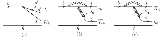
Figure 1: Three different penguin contributions to $\overline{B}\to\overline{K}_{h}\eta^{(^{\prime})}$ with $K_{h}$ denoting $K,K^{*},K_{0}^{*}(1430)$ and $K_{2}^{*}(1430)$. Fig. 1(a) is induced by the penguin operators $O_{3,5,7,9}$.

I Introduction

Recently BaBar has measured charmless $B$ decays with final states containing $\eta$ or $\eta^{\prime}$ BaBar:Keta . Comparing the first measurements of $B\to K_{0}^{*}(1430)\eta^{\prime}$ and $B\to K_{2}^{*}(1430)\eta^{\prime}$ by BaBar with previous results of $B\to K_{0}^{*}(1430)\eta$ and $B\to K_{2}^{*}(1430)\eta$ (see Table 1) clearly indicates that ${\cal B}(B\to K_{0}^{*}(1430)\eta^{\prime})<{\cal B}(B\to K_{0}^{*}(1430)\eta)$ and ${\cal B}(B\to K_{2}^{*}(1430)\eta^{\prime})>{\cal B}(B\to K_{2}^{*}(1430)\eta)$. It is well known that ${\cal B}(B\to K\eta^{\prime})\gg{\cal B}(B\to K\eta)$ and ${\cal B}(B\to K^{*}\eta^{\prime})\ll{\cal B}(B\to K^{*}\eta)$. The last two patterns can be understood as the interference between the dominant penguin amplitudes.

Table 1: Experimental branching fractions (in units of $10^{-6}$) of $B\to K_{h}\eta^{(^{\prime})}$ with $K_{h}=K,K^{*},K_{0}^{*}(1430)$ and $K_{2}^{*}(1430)$ taken from HFAG ; BaBar:Keta .

	$K\eta$	$K\eta^{\prime}$	$K^{*}\eta$	$K^{*}\eta^{\prime}$	$K_{0}^{*}\eta$	$K_{0}^{*}\eta^{\prime}$	$K_{2}^{*}\eta$	$K_{2}^{*}\eta^{\prime}$
$B^{+}$	$2.36\pm 0.27$	$71.1\pm 2.6$	$19.3\pm 1.6$	$4.9^{+2.1}_{-1.9}$	$15.8\pm 3.1$	$5.2\pm 2.1$	$9.1\pm 3.0$	$28.0^{+5.3}_{-5.0}$
$B^{0}$	$1.12^{+0.30}_{-0.28}$	$66.1\pm 3.1$	$15.9\pm 1.0$	$3.8\pm 1.2$	$9.6\pm 1.9$	$6.3\pm 1.6$	$9.6\pm 2.1$	$13.7^{+3.2}_{-3.1}$

For the $\eta$ and $\eta^{\prime}$ particles, it is more convenient to consider the flavor states $q\bar{q}\equiv(u\bar{u}+d\bar{d})/\sqrt{2}$, $s\bar{s}$ and $c\bar{c}$ labeled by the $\eta_{q}$, $\eta_{s}$ and $\eta_{c}^{0}$, respectively. Neglecting the small mixing with $\eta_{c}^{0}$, we write

$$\left(\begin{array}[]{c}|\eta\rangle\\ |\eta^{\prime}\rangle\end{array}\right)=\left(\begin{array}[]{ccc}\cos\phi&-\sin\phi\\ \sin\phi&\cos\phi\end{array}\right)\left(\begin{array}[]{c}|\eta_{q}\rangle\\ |\eta_{s}\rangle\end{array}\right)\;,$$ (1)

where $\phi=(39.3\pm 1.0)^{\circ}$ FKS is the $\eta-\eta^{\prime}$ mixing angle in the $\eta_{q}$ and $\eta_{s}$ flavor basis. Three different penguin contributions are depicted in Fig. 1: (i) $b\to sq\bar{q}\to s\eta_{q}$, (ii) $b\to ss\bar{s}\to s\eta_{s}$, and (iii) $b\to sq\bar{q}\to q\bar{K}_{h}$, corresponding to Figs. 1(a), 1(b) and 1(c), respectively. For $B\to K^{(*)}\eta^{(^{\prime})}$ decays, the dominant penguin amplitudes arise from Figs. 1(b) and 1(c) governed by the parameters $\alpha_{4}(K_{h}\eta_{s})$ and $\alpha_{4}(\eta_{q}K_{h})$, respectively. Their expressions in terms of the effective Wilson coefficients $a_{4}$ and $a_{6}$ are summarized in Table 2.

It is clear that the interference between the $B\to K\eta_{q}$ amplitude induced by the $b\to sq\bar{q}$ penguin and the $B\to K\eta_{s}$ amplitude induced by $b\to ss\bar{s}$ is constructive for $B\to K\eta^{\prime}$ and destructive for $B\to K\eta$. This explains the large rate of the former and the suppression of the latter Lipkin . For $B\to K^{*}\eta^{(^{\prime})}$ decays, it is the other way around. The sign difference between $\alpha_{4}(\eta_{q}K^{*})$ and $\alpha_{4}(K^{*}\eta_{s})$ explains why $\Gamma(B\to K^{*}\eta)\gg\Gamma(B\to K^{*}\eta^{\prime})$, recalling that $a_{4}$ and $a_{6}$ are negative and the magnitude of the latter is larger than the former and that the chiral factor $r_{\chi}$ to be defined below is of order unity for light mesons.

The decay pattern for $B\to K_{0}^{*}(1430)\eta^{(^{\prime})}$ decays depends on whether $K_{0}^{*}(1430)$ is an excited state of $\kappa$ (or $K_{0}^{*}(800)$) or a low lying $P$-wave $q\bar{q}$ state. Hence, the experimental measurements of $B\to K_{0}^{*}(1430)\eta^{(^{\prime})}$ can be used to explore the quark structure of the scalar meson $K_{0}^{*}(1430)$. A detailed study in this work shows that $\Gamma(B\to K_{0}^{*}\eta)\ll\Gamma(B\to K^{*}_{0}\eta^{\prime})$ in the first scenario for $K_{0}^{*}(1430)$ and $\Gamma(B\to K_{0}^{*}\eta)>\Gamma(B\to K^{*}_{0}\eta^{\prime})$ in the latter scenario. As for $B\to K_{2}^{*}(1430)\eta^{(^{\prime})}$ decays, Fig. 1(c) does not make contribution owing to the vanishing decay constant of $K_{2}^{*}$. Since the interference between Figs. 1(a) and 1(b) is constructive for $K_{2}^{*}\eta^{\prime}$ and destructive for $K_{2}^{*}\eta$ and since the decay constant $f_{\eta^{\prime}}^{s}$ is larger than $f_{\eta}^{s}$, one will expect a larger rate for $K_{2}^{*}\eta^{\prime}$ than $K_{2}^{*}\eta$.

Table 2: The parameters $\alpha_{4}(K_{h}\eta_{s})$ and $\alpha_{4}(\eta_{q}K_{h})$ with $K_{h}=K,K^{*},K_{0}^{*}(1430)$ and $K_{2}^{*}(1430)$.

	$K$	$K^{*}$	$K_{0}^{*}(1430)$	$K_{2}^{*}(1430)$
$\alpha_{4}(K_{h}\eta_{s})$	$a_{4}+r_{\chi}^{\eta_{s}}a_{6}$	$a_{4}-r_{\chi}^{\eta_{s}}a_{6}$	$a_{4}-r_{\chi}^{\eta_{s}}a_{6}$	$a_{4}-r_{\chi}^{\eta_{s}}a_{6}$
$\alpha_{4}(\eta_{q}K_{h})$	$a_{4}+r_{\chi}^{K}a_{6}$	$a_{4}+r_{\chi}^{K^{*}}a_{6}$	$a_{4}-r_{\chi}^{K_{0}^{*}}a_{6}$	$-$

Recently we have studied the decays $B\to(K,K^{*})\eta^{(^{\prime})}$ within the framework of QCD factorization (QCDF) CC:Bud ; CC:BCP . Here we shall present updated results with some discussions. Then in the rest of this work we will focus on $B\to(K_{0}^{*}(1430),K^{*}_{2}(1430))\eta^{(^{\prime})}$ decays and study their decay pattern.

The layout of the present paper is as follows. In Sec. II we recapitulate the framework of QCD factorization. The we proceed to study $B\to(K,K^{*})(\eta,\eta^{\prime})$ decays in Sec. III and $B\to K_{0}^{*}(1430)(\eta,\eta^{\prime})$ decays in Sec. IV. Since the QCDF approach for the $K_{2}^{*}(1430)\eta^{(^{\prime})}$ modes has not been developed, we reply on naive factorization to study the tensor meson production in Sec. V. Sec. VI comes to our conclusions. An appendix is devoted to the decay constants and matrix elements of the $\eta$ and $\eta^{\prime}$ mesons.

II QCD factorization

Within the framework of QCDF BBNS , the effective Hamiltonian matrix elements are written in the form

$$\langle M_{1}M_{2}|{\cal H}_{\rm eff}|\overline{B}\rangle\!=\!\frac{G_{F}}{\sqrt{2}}\sum_{p=u,c}\!\lambda_{p}^{(q)}\,\!\langle M_{1}M_{2}|{\cal T_{A}}^{p}\!+\!{\cal T_{B}}^{p}|\overline{B}\rangle\,,$$ (2)

where $\lambda_{p}^{(q)}=V_{pb}V_{pq}^{*}$ with $q=s,d$, ${\cal T_{A}}$ describes contributions from naive factorization, vertex corrections, penguin contractions and spectator scattering expressed in terms of the flavor operators $a_{i}^{p}$, while ${\cal T_{B}}$ contains annihilation topology amplitudes characterized by the annihilation operators $b_{i}^{p}$. The explicit expressions of ${\cal T_{A}}$ and ${\cal T_{B}}$ can be found in BN ; BBNS . In practice, it is more convenient to express the decay amplitudes in terms of the flavor operators $\alpha_{i}^{p}$ and the annihilation operators $\beta_{i}^{p}$. Their relations to the coefficients $a_{i}^{p}$ and $b_{i}^{p}$ will be specified below.

The expressions of $\bar{B}\to\bar{K}_{h}\eta^{(^{\prime})}$ decay amplitudes for $K_{h}=K,K^{*},K_{0}^{*}(1430)$ and $K_{2}^{*}(1430)$ are given by BN

$$\sqrt{2}A_{B^{-}\to K_{h}^{-}\eta^{(^{\prime})}} = X^{(\bar{B}\bar{K}_{h},\eta^{(^{\prime})}_{q})}\left[\delta_{pu}(\alpha_{2}+2\beta_{S2})+2\alpha_{3}^{p}+{1\over 2}\alpha^{p}_{3,EW}+2\beta^{p}_{S3}+2\beta^{p}_{S3,EW}\right]$$ (3)

$$+ \sqrt{2}X^{(\bar{B}\bar{K}_{h},\eta^{(^{\prime})}_{s})}\Big{[}\delta_{pu}(\beta_{2}+2\beta_{S2})+\alpha_{3}^{p}+\alpha_{4}^{p}-{1\over 2}\alpha^{p}_{3,EW}-{1\over 2}\alpha^{p}_{4,EW}+\beta^{p}_{3}+\beta^{p}_{3,EW}$$

$$+ \beta_{S3}^{p}+\beta^{p}_{S3,EW}\Big{]}+\sqrt{2}X^{(\bar{B}\bar{K}_{h},\eta^{(^{\prime})}_{c})}\left[\delta_{pc}\alpha_{2}+\alpha_{3}^{p}\right]$$

$$+ X^{(\bar{B}\eta^{(^{\prime})}_{q},\bar{K}_{h})}\left[\delta_{pu}(\alpha_{1}+\beta_{2})+\alpha_{4}^{p}+\alpha^{p}_{4,EW}+\beta_{3}^{p}+\beta^{p}_{3,EW}\right],$$

$$\sqrt{2}A_{\bar{B}^{0}\to\bar{K}_{h}^{0}\eta^{(^{\prime})}} = X^{(\bar{B}\bar{K}_{h},\eta^{(^{\prime})}_{q})}\left[\delta_{pu}\alpha_{2}+2\alpha_{3}^{p}+{1\over 2}\alpha^{p}_{3,EW}+2\beta^{p}_{S3}-\beta^{p}_{S3,EW}\right]$$

$$+ \sqrt{2}X^{(\bar{B}\bar{K}_{h},\eta^{(^{\prime})}_{s})}\Big{[}\alpha_{3}^{p}+\alpha_{4}^{p}-{1\over 2}\alpha^{p}_{3,EW}-{1\over 2}\alpha^{p}_{4,EW}+\beta^{p}_{3}-{1\over 2}\beta^{p}_{3,EW}+\beta_{S3}^{p}-{1\over 2}\beta^{p}_{S3,EW}\Big{]}$$

$$+ \sqrt{2}X^{(\bar{B}\bar{K}_{h},\eta^{(^{\prime})}_{c})}\left[\delta_{pc}\alpha_{2}+\alpha_{3}^{p}\right]+X^{(\bar{B}\eta^{(^{\prime})}_{q},\bar{K}_{h})}\left[\alpha_{4}^{p}-{1\over 2}\alpha^{p}_{4,EW}+\beta_{3}^{p}-{1\over 2}\beta^{p}_{3,EW}\right].$$

The order of the arguments of $\alpha_{i}^{p}(M_{1}M_{2})$ and $\beta_{i}^{p}(M_{1}M_{2})$, which are not shown explicitly here, is consistent with the order of the arguments of the factorizable matrix elements $X^{(\overline{B}M_{1},M_{2})}$ given by

$$X^{(\bar{B}P_{1},P_{2})} \equiv \langle P_{2}|J^{\mu}|0\rangle\langle P_{1}|J^{\prime}_{\mu}|\overline{B}\rangle=if_{P_{2}}(m_{B}^{2}-m^{2}_{P_{1}})F_{0}^{BP_{1}}(m_{P_{2}}^{2}),$$

$$X^{(\bar{B}P,V)} \equiv \langle V|J^{\mu}|0\rangle\langle P|J^{\prime}_{\mu}|\overline{B}\rangle=2f_{V}\,m_{B}p_{c}F_{1}^{BP}(m_{V}^{2}),$$

$$X^{(\bar{B}V,P)} \equiv \langle P|J^{\mu}|0\rangle\langle V|J^{\prime}_{\mu}|\overline{B}\rangle=2f_{P}\,m_{B}p_{c}A_{0}^{BV}(m_{P}^{2}),$$ (4)

$$X^{(\bar{B}P,S)} \equiv \langle S|J^{\mu}|0\rangle\langle P|J^{\prime}_{\mu}|\overline{B}\rangle=f_{S}\,(m_{B}^{2}-m_{P}^{2})F_{0}^{BP}(m_{S}^{2}),$$

$$X^{(\bar{B}S,P)} \equiv \langle P|J^{\mu}|0\rangle\langle S|J^{\prime}_{\mu}|\overline{B}\rangle=-f_{P}\,(m_{B}^{2}-m_{S}^{2})F_{0}^{BS}(m_{P}^{2}),$$

$$X^{(\bar{B}T,P)} \equiv \langle P|J^{\mu}|0\rangle\langle T|J^{\prime}_{\mu}|\overline{B}\rangle=-if_{P}[k(m_{P}^{2})+(m_{B}^{2}-m_{T}^{2})b_{+}(m_{P}^{2})+m_{P}^{2}b_{-}(m_{P}^{2})]\varepsilon^{*}_{\mu\nu}p_{B}^{\mu}p_{B}^{\nu},$$

$$X^{(\bar{B}P,T)} \equiv \langle T|J^{\mu}|0\rangle\langle P|J^{\prime}_{\mu}|\overline{B}\rangle=0,$$

where $f_{P},f_{V},f_{S}$ are the decay constants of pseudoscalar, vector and scalar mesons, respectively, and $k,b_{+},b_{-}$ are $B$ to tensor meson transition form factors defined in Eq. (38) below.

The flavor operators $\alpha_{i}^{p}$ and the annihilation operators $\beta_{i}^{p}$ are related to the coefficients $a_{i}^{p}$ and $b_{i}^{p}$ by

$$\alpha_{1}(M_{1}M_{2}) = a_{1}(M_{1}M_{2})\,,$$

$$\alpha_{2}(M_{1}M_{2}) = a_{2}(M_{1}M_{2})\,,$$

$$\alpha_{3}^{p}(M_{1}M_{2}) = \left\{\begin{array}[]{cl}a_{3}^{p}(M_{1}M_{2})-a_{5}^{p}(M_{1}M_{2})&\quad\mbox{for~{}}M_{1}M_{2}=PP,\,VP,\,SP,\,TP\\ a_{3}^{p}(M_{1}M_{2})+a_{5}^{p}(M_{1}M_{2})&\quad\mbox{for~{}}M_{1}M_{2}=PV,\,PS,\end{array}\right.$$ (7)

$$\alpha_{4}^{p}(M_{1}M_{2}) = \left\{\begin{array}[]{cl}a_{4}^{p}(M_{1}M_{2})+r_{\chi}^{M_{2}}\,a_{6}^{p}(M_{1}M_{2})&\quad\mbox{for~{}}M_{1}M_{2}=PP,\,PV,\\ a_{4}^{p}(M_{1}M_{2})-r_{\chi}^{M_{2}}\,a_{6}^{p}(M_{1}M_{2})&\quad\mbox{for~{}}M_{1}M_{2}=VP,\,SP,\,PS,\,TP\end{array}\right.$$ (10)

$$\alpha_{3,\rm EW}^{p}(M_{1}M_{2}) = \left\{\begin{array}[]{cl}a_{9}^{p}(M_{1}M_{2})-a_{7}^{p}(M_{1}M_{2})&\quad\mbox{for~{}}M_{1}M_{2}=PP,\,VP,\,SP,\,TP\\ a_{9}^{p}(M_{1}M_{2})+a_{7}^{p}(M_{1}M_{2})&\quad\mbox{for~{}}M_{1}M_{2}=PV,\,PS,\end{array}\right.$$ (13)

$$\alpha_{4,\rm EW}^{p}(M_{1}M_{2}) = \left\{\begin{array}[]{cl}a_{10}^{p}(M_{1}M_{2})+r_{\chi}^{M_{2}}\,a_{8}^{p}(M_{1}M_{2})&\quad\mbox{for~{}}M_{1}M_{2}=PP,\,PV,\\ a_{10}^{p}(M_{1}M_{2})-r_{\chi}^{M_{2}}\,a_{8}^{p}(M_{1}M_{2})&\quad\mbox{for~{}}M_{1}M_{2}=VP\,,SP,\,PS,\,TP\end{array}\right.$$ (16)

and

$$\beta_{i}^{p}(M_{1}M_{2})=\frac{if_{B}f_{M_{1}}f_{M_{2}}}{X^{(\overline{B}M_{1},M_{2})}}b_{i}^{p},$$ (17)

where the chiral factors $r_{\chi}$’s are given by

$$r_{\chi}^{P}(\mu)={2m_{P}^{2}\over m_{b}(\mu)(m_{2}+m_{1})(\mu)},\quad r_{\chi}^{\eta_{s}}={h_{P}^{s}\over f_{P}^{s}m_{b}(\mu)m_{s}(\mu)},$$

$$r_{\chi}^{V}(\mu)=\frac{2m_{V}}{m_{b}(\mu)}\,\frac{f_{V}^{\perp}(\mu)}{f_{V}},\qquad\qquad r_{\chi}^{K_{0}^{*}}(\mu)={2m_{K_{0}^{*}}^{2}\over m_{b}(\mu)(m_{s}-m_{q})(\mu)},$$ (18)

with the parameters $f_{P}^{s}$ and $h_{P}^{s}$ being defined in the Appendix.

The flavor operators $a_{i}^{p}$ are basically the Wilson coefficients in conjunction with short-distance nonfactorizable corrections such as vertex corrections and hard spectator interactions. In general, they have the expressions BBNS ; BN

$$a_{i}^{p}(M_{1}M_{2})=\left(c_{i}+{c_{i\pm 1}\over N_{c}}\right)N_{i}(M_{2})+{c_{i\pm 1}\over N_{c}}\,{C_{F}\alpha_{s}\over 4\pi}\Big{[}V_{i}(M_{2})+{4\pi^{2}\over N_{c}}H_{i}(M_{1}M_{2})\Big{]}+P_{i}^{p}(M_{2}),$$ (19)

where $i=1,\cdots,10$, the upper (lower) signs apply when $i$ is odd (even), $c_{i}$ are the Wilson coefficients, $C_{F}=(N_{c}^{2}-1)/(2N_{c})$ with $N_{c}=3$, $M_{2}$ is the emitted meson and $M_{1}$ shares the same spectator quark with the $B$ meson. The quantities $V_{i}(M_{2})$ account for vertex corrections, $H_{i}(M_{1}M_{2})$ for hard spectator interactions with a hard gluon exchange between the emitted meson and the spectator quark of the $B$ meson and $P_{i}(M_{2})$ for penguin contractions. The expression of the quantities $N_{i}(M_{2})$ reads

$$N_{i}(M_{2})=\cases{0,&$i=6,8$ and $M_{2}=V$,\cr 1,&{\rm else}.\cr}$$ (20)

In Eq. (3), possible flavor-singlet penguin annihilation contributions are denoted by $\beta_{S}$’s which will not be considered in this work.

Power corrections in QCDF always involve troublesome endpoint divergences. For example, the annihilation amplitude has endpoint divergences even at twist-2 level and the hard spectator scattering diagram at twist-3 order is power suppressed and posses soft and collinear divergences arising from the soft spectator quark. Since the treatment of endpoint divergences is model dependent, subleading power corrections generally can be studied only in a phenomenological way. We shall follow BBNS to model the endpoint divergence $X\equiv\int^{1}_{0}dx/(1-x)$ in the annihilation and hard spectator scattering diagrams as

$$X_{A}=\ln\left({m_{B}\over\Lambda_{h}}\right)(1+\rho_{A}e^{i\phi_{A}}),\qquad X_{H}=\ln\left({m_{B}\over\Lambda_{h}}\right)(1+\rho_{H}e^{i\phi_{H}}),$$ (21)

with $\Lambda_{h}$ being a typical scale of order 500 MeV, and $\rho_{A,H}$, $\phi_{A,H}$ being the unknown real parameters.

As pointed out in CC:BCP , while the discrepancies between experiment and theory in the heavy quark limit for the rates of penguin-dominated two-body decays of $B$ mesons and direct CP asymmetries of $\bar{B}^{0}\to K^{-}\pi^{+}$, $B^{-}\to K^{-}\rho^{0}$ and $\bar{B}^{0}\to\pi^{+}\pi^{-}$ are resolved by introducing power corrections coming from penguin annihilation, the signs of direct CP-violating effects in $B^{-}\to K^{-}\pi^{0},B^{-}\to K^{-}\eta$ and $\bar{B}^{0}\to\pi^{0}\pi^{0}$ are flipped to the wrong ones when confronted with experiment. These new $B$-CP puzzles in QCDF can be resolved by the subleading power corrections to the color-suppressed tree amplitudes due to spectator interactions and/or final-state interactions Chua that not only reproduce correct signs for aforementioned CP asymmetries but also accommodate the observed $\bar{B}_{d}\to\pi^{0}\pi^{0}$ and $\rho^{0}\pi^{0}$ rates simultaneously. Following CC:BCP , power corrections to the color-suppressed topology are parametrized as

$$a_{2}\to a_{2}(1+\rho_{C}e^{i\phi_{C}}),$$ (22)

with the unknown parameters $\rho_{C}$ and $\phi_{C}$ to be inferred from experiment.

For $S$-wave mesons, input parameters such as decay constants, form factors, quark masses, Wolfenstein parameters, light-cone distribution amplitudes, power correction parameters can be found in CC:Bud . Input parameters for parity-even mesons such as $K_{0}^{*}(1430)$ and $K_{2}^{*}(1430)$ will be specified later. For the renormalization scale of the decay amplitude, we choose $\mu=m_{b}(m_{b})=4.2$ GeV.

III $B\to(K,K^{*})(\eta,\eta^{\prime})$ decays

Table 3: Branching fractions (top; in units of $10^{-6}$) and direct CP asymmetries (bottom; in units of %) of $B\to(K,K^{*})(\eta,\eta^{\prime})$ decays obtained in various approaches. The pQCD results are taken from XiaoKeta for $B\to K\eta^{(^{\prime})}$ with partial NLO corrections and from ChenKeta for $B\to K^{*}\eta^{(^{\prime})}$. There are two solution sets with SCET predictions for decays involving $\eta$ and/or $\eta^{\prime}$ Zupan ; SCETVP . The theoretical errors correspond to the uncertainties due to the variation of (i) Gegenbauer moments, decay constants, quark masses, form factors, the $\lambda_{B}$ parameter for the $B$ meson wave function, and (ii) $\rho_{A,H}$, $\phi_{A,H}$, respectively.

Mode	QCDF (this work)	pQCD	SCET	Expt. HFAG ; BaBar:Keta
$B^{-}\to K^{-}\eta$	$2.2^{+1.7+1.1}_{-1.0-0.9}$	$3.2^{+1.2+2.7+1.1}_{-0.9-1.2-1.0}$	$2.7\pm 4.8\pm 0.4\pm 0.3$	$2.36\pm 0.27$
			$2.3\pm 4.5\pm 0.4\pm 0.3$
$B^{-}\to K^{-}\eta^{\prime}$	$74.5^{+57.9+25.6}_{-25.3-19.0}$	$51.0^{+13.5+11.2+4.2}_{-~{}8.2-~{}\,6.2-3.5}$	$69.5\pm 27.0\pm 4.4\pm 7.7$	$71.1\pm 2.6$
			$69.3\pm 26.0\pm 7.1\pm 6.3$
$\bar{B}^{0}\to\bar{K}^{0}\eta$	$1.5^{+1.4+0.9}_{-0.8-0.7}$	$2.1^{+0.8+2.3+1.0}_{-0.6-1.0-0.9}$	$2.4\pm 4.4\pm 0.2\pm 0.3$	$1.12^{+0.30}_{-0.28}$
			$2.3\pm 4.4\pm 0.2\pm 0.5$
$\bar{B}^{0}\to\bar{K}^{0}\eta^{\prime}$	$70.9^{+54.1+24.2}_{-23.8-18.0}$	$50.3^{+11.8+11.1+4.5}_{-~{}8.2-~{}6.2-2.7}$	$63.2\pm 24.7\pm 4.2\pm 8.1$	$66.1\pm 3.1$
			$62.2\pm 23.7\pm 5.5\pm 7.2$
$B^{-}\to K^{*-}\eta$	$15.8^{+8.2+9.6}_{-4.2-7.3}$	$22.13^{+0.26}_{-0.27}$	$17.9_{-5.4-2.9}^{+5.5+3.5}$	$19.3\pm 1.6$
			$18.6_{-4.8-2.2}^{+4.5+2.5}$
$B^{-}\to K^{*-}\eta^{\prime}$	$1.6^{+2.1+3.7}_{-0.3-1.6}$	$6.38\pm 0.26$	$4.5_{-3.9-0.8}^{+6.6+0.9}$	$4.8^{+1.8}_{-1.6}$
			$4.8_{-3.7-0.6}^{+5.3+0.8}$
$\bar{B}^{0}\to\bar{K}^{*0}\eta$	$15.7^{+7.7+9.6}_{-4.0-7.3}$	$22.31^{+0.28}_{-0.29}$	$16.6_{-5.0-2.7}^{+5.1+3.2}$	$15.9\pm 1.0$
			$16.5_{-4.3-2.0}^{+4.1+2.3}$
$\bar{B}^{0}\to\bar{K}^{*0}\eta^{\prime}$	$1.5^{+1.8+3.5}_{-0.3-1.6}$	$3.35^{+0.29}_{-0.27}$	$4.1_{-3.6-0.7}^{+6.2+0.9}$	$3.1^{+1.0}_{-0.9}$
			$4.0_{-3.4-0.6}^{+4.7+0.7}$
$B^{-}\to K^{-}\eta$	$-14.5^{+10.3+15.5}_{-26.0-10.7}$	$-11.7^{+6.8+3.9+2.9}_{-9.6-4.2-5.6}$	$33\pm 30\pm 7\pm 3$	$-37\pm 9$
			$-33\pm 39\pm 10\pm 4$
$B^{-}\to K^{-}\eta^{\prime}$	$0.45^{+0.69+1.20}_{-0.55-0.98}$	$-6.2^{+1.2+1.3+1.3}_{-1.1-1.0-1.0}$	$-10\pm 6\pm 7\pm 5$	$1.3^{+1.6}_{-1.7}$
			$0.7\pm 0.5\pm 0.2\pm 0.9$
$\bar{B}^{0}\to\bar{K}^{0}\eta$	$-23.6^{+~{}9.8+12.6}_{-26.2-12.5}$	$-12.7^{+4.1+3.2+3.2}_{-4.1-1.5-6.7}$	$21\pm 20\pm 4\pm 3$
			$-18\pm 22\pm 6\pm 4$
$\bar{B}^{0}\to\bar{K}^{0}\eta^{\prime}$	$3.0^{+0.6+0.8}_{-0.5-0.8}$	$2.3^{+0.5+0.3+0.2}_{-0.4-0.6-0.1}$	$11\pm 6\pm 12\pm 2$	$5\pm 5$
			$-27\pm 7\pm 8\pm 5$
$B^{-}\to K^{*-}\eta$	$-10.1^{+3.9+6.5}_{-3.7-7.8}$	$-24.57^{+0.72}_{-0.27}$	$-2.6_{-5.5-0.3}^{+5.4+0.3}$	$2\pm 6$
			$-1.9_{-3.6-0.1}^{+3.4+0.1}$
$B^{-}\to K^{*-}\eta^{\prime}$	$69.7^{+~{}6.5+27.9}_{-38.6-49.5}$	$4.60^{+1.16}_{-1.32}$	$2.7_{-19.5-0.3}^{+27.4+0.4}$	$-26\pm 27$
			$2.6_{-32.9-0.2}^{+26.7+0.2}$
$\bar{B}^{0}\to\bar{K}^{*0}\eta$	$3.4^{+0.4+2.7}_{-0.4-2.4}$	$0.57\pm 0.011$	$-1.1_{-2.4-0.1}^{+2.3+0.1}$	$19\pm 5$
			$-0.7_{-1.3-0.0}^{+1.2+0.1}$
$\bar{B}^{0}\to\bar{K}^{*0}\eta^{\prime}$	$8.8^{+~{}8.8+30.8}_{-10.7-24.1}$	$-1.30\pm 0.08$	$9.6_{-11.0-1.2}^{+~{}8.9+1.3}$	$2\pm 23$
			$9.9_{-4.3-0.9}^{+6.2+0.9}$

III.1 Branching fractions

Details of the calculations in the framework of QCDF for all $B\to PP,VP$ decays can be found in CC:Bud ; CC:BCP . The updated results for the branching fractions and direct CP asymmetries in $B\to K^{(*)}\eta^{(^{\prime})}$ decays are exhibited in Table 3 after correcting some minor errors in the previous computer codes.

Numerically, Beneke and Neubert already obtained ${\cal B}(B^{-}\to K^{-}\eta^{\prime})\sim{\cal O}(50\times 10^{-6})$ in QCDF using the default values $\rho_{A}=\rho_{H}=0$ BN . Here we found similar results $57\times 10^{-6}$ ($53\times 10^{-6}$) with (without) the contributions from the “charm content” of the $\eta^{\prime}$. In the presence of penguin annihilation, we obtain ${\cal B}(B^{-}\to K^{-}\eta^{\prime})\sim 75\times 10^{-6}$ ($67\times 10^{-6}$) with (without) the “charm content” contributions. Therefore, the observed large $B\to K\eta^{\prime}$ rates are naturally explained in QCDF without invoking, for example, significant flavor-singlet contributions or an enhanced hadronic matrix element $\langle 0|\bar{s}\gamma_{5}s|\eta^{\prime}\rangle$. Data on $B\to K\eta$ modes are also well accounted for by QCDF.

The values of the parameters $\alpha_{4}(K^{(*)}\eta_{q,s})$ and $\alpha_{4}(\eta_{q}K^{(*)})$ are given by

$$\alpha_{4}(K\eta_{s})=-0.098-0.013i, \alpha_{4}(\eta_{q}K)=-0.094-0.013i,$$

$$\alpha_{4}(K^{*}\eta_{s})=0.035-0.0009i, \alpha_{4}(\eta_{q}K^{*})=-0.036-0.0085i.$$ (23)

The magnitude of $\alpha_{4}(\eta_{q}K^{*})$ is smaller than $\alpha_{4}(\eta_{q}K)$ owing to the smallness of $r_{\chi}^{K^{*}}\sim 0.36$ compared to $r_{\chi}^{K}\sim 1.45$ at the scale $\mu=4.2$ GeV, while the smallness of $\alpha_{4}(K^{*}\eta_{s})$ relative to $\alpha_{4}(K\eta_{s})$ is due to the destructive interference in the former. The sign difference between $\alpha_{4}(\eta_{q}K^{*})$ and $\alpha_{4}(K^{*}\eta_{s})$ explains why $\Gamma(B\to K^{*}\eta)\gg\Gamma(B\to K^{*}\eta^{\prime})$. Although the rates of $K^{*}\eta^{\prime}$ and $K\eta$ are comparable, ${\cal B}(B\to K^{*}\eta)$ is much smaller than ${\cal B}(B\to K\eta^{\prime})$.

The QCDF prediction for the branching fraction of $B\to K^{*}\eta^{\prime}$, of order $1.5\times 10^{-6}$, is smaller than the predictions of pQCD and soft-collinear effective theory (SCET), but it is consistent with experiment within errors. The experimental values quoted in Table 3 are the BaBar measurements BaBar:Keta . Belle obtained only the upper bounds: ${\cal B}(B^{-}\to K^{*-}\eta^{\prime})<2.9\times 10^{-6}$ and ${\cal B}(\bar{B}^{0}\to\bar{K}^{*0}\eta^{\prime})<2.6\times 10^{-6}$ Belle:Ksteta' . Therefore, although our central values are smaller than BaBar, they are consistent with Belle. It is very important to measure them to discriminate between various model predictions.

III.2 ${\it CP}~{}$ asymmetries

There are two modes in which direct CP asymmetries have been measured with significance around $4\sigma$ : $A_{CP}(K^{-}\eta)=-0.37\pm 0.09$ and $A_{CP}(\bar{K}^{*0}\eta)=0.19\pm 0.05$. It is crucial to understand them. Since the two penguin diagrams Figs. 1(b) and 1(c) contribute destructively to $B\to K\eta$ due to the opposite sign of $f_{\eta}^{q}$ and $f_{\eta}^{s}$, the penguin amplitude is comparable in magnitude to the tree amplitude induced from $b\to us\bar{u}$, contrary to the decay $B\to K\eta^{\prime}$ which is dominated by large penguin amplitudes. Consequently, a sizable direct CP asymmetry is expected in $B^{-}\to K^{-}\eta$ but not in $K^{-}\eta^{\prime}$ BSS .

In the absence of any power corrections, it appears that the QCDF prediction $A_{CP}(K^{-}\eta)=-0.233^{+0.164}_{-0.193}$ obtained in the leading $1/m_{b}$ expansion already agrees well with the data. However, this agreement is just an accident. Recall that when power corrections are turned off, the predicted CP asymmetries for the penguin-dominated modes $K^{-}\pi^{+}$, $K^{*-}\pi^{+}$, $K^{-}\rho^{+}$, $K^{-}\rho^{0}$, and tree-dominated modes $\pi^{+}\pi^{-}$, $\rho^{\pm}\pi^{\mp}$ and $\rho^{-}\pi^{+}$ are wrong in signs when confronted with experiment CC:Bud ; CC:BCP . That is why it is important to consider the effects of power corrections step by step. The QCDF results in the heavy quark limit should not be considered as the final QCDF predictions to be compared with experiment. It turns out that the aforementioned wrong signs can be flipped into the right direction by the power corrections from penguin annihilation.

However, a scrutiny of the QCDF predictions reveals more puzzles with respect to direct CP violation. While the signs of CP asymmetries in $K^{-}\pi^{+},K^{-}\rho^{0}$ modes etc., are flipped to the right ones in the presence of power corrections from penguin annihilation, the signs of $A_{CP}$ in $B^{-}\to K^{-}\pi^{0},~{}K^{-}\eta,~{}\pi^{-}\eta$ and $\bar{B}^{0}\to\pi^{0}\pi^{0},~{}\bar{K}^{*0}\eta$ will also get reversed in such a way that they disagree with experiment CC:Bud ; CC:BCP . Specifically, $A_{CP}(K^{-}\eta)$ is found to be of order $0.11$ in the presence of penguin annihilation and hence it has a wrong sign. These CP puzzles can be resolved by having soft corrections to the color-suppressed tree coefficient $a_{2}$ so that $a_{2}$ is large and complex. When $\rho_{C}$ and $\phi_{C}$ are turned on (see Eq. (22) with $\rho_{C}=1.3$ and $\phi_{C}=-70^{\circ}$ CC:Bud ), $A_{CP}(K^{-}\eta)$ will be reduced to $-0.02$ if there is no intrinsic charm content of the $\eta$. Although the decay constant $f_{\eta}^{c}\approx-2$ MeV is much smaller than $f_{\eta}^{q,s}$ [see Eq. (A)], its effect is CKM enhanced by $V_{cb}V_{cs}^{*}/(V_{ub}V_{us}^{*})$. Therefore, the charm content of the $\eta$ may have a significant impact on CP violation. Indeed, when $f_{\eta}^{c}$ is turned on, $A_{CP}(K^{-}\eta)$ finally reaches the level of $-15\%$ with a sign in agreement with experiment. Hence, CP asymmetry in $B^{-}\to K^{-}\eta$ is the place where the charm content of the $\eta$ plays a role. The pQCD prediction is similar to QCDF. For comments on the pQCD calculation of $A_{CP}(K^{-}\eta)$, the reader is referred to CC:Bud . Note that while both QCDF and pQCD lead to a correct sign for $A_{CP}(K^{-}\eta)$, the predicted magnitude still falls short of the measurement $-0.37\pm 0.09$.

As for CP asymmetry in $\bar{B}^{0}\to\bar{K}^{*0}\eta$, we have $A_{CP}(\bar{K}^{*0}\eta)=(3.1^{+2.0}_{-1.9})\%$ in the heavy quark limit. It is modified to $(0.12^{+2.10}_{-1.60})\%$ by penguin annihilation. Soft corrections to the color-suppressed tree amplitude is needed to improve the prediction and finally we obtain $A_{CP}(\bar{K}^{*0}\eta)=(3.4^{+2.8}_{-2.4})\%$ (Table 3). Unlike the $K^{0}\eta$ mode, the charm content of the $\eta$ here does not play an essential role for CP violation in $K^{*0}\eta$. We see from Table 3 that QCDF is in better agreement with experiment than pQCD and SCET, though it is still smaller than the data.

IV $B\to K_{0}^{*}(1430)\eta^{(^{\prime})}$ decays in QCDF

The hadronic charmless $B$ decays into a scalar meson and a pseudoscalar meson have been studied in QCDF in CCY:SP . For scalar mesons above 1 GeV we have explored two possible scenarios in the QCD sum rule method, depending on whether the light scalars $\kappa,~{}a_{0}(980)$ and $f_{0}(980)$ are treated as the lowest lying $q\bar{q}$ states or four-quark particles: (i) In scenario 1, we treat $\kappa,a_{0}(980),f_{0}(980)$ as the lowest lying states, and $K_{0}^{*}(1430),a_{0}(1450),f_{0}(1500)$ as the corresponding first excited states, respectively, and (ii) we assume in scenario 2 that $K_{0}^{*}(1430),a_{0}(1450),f_{0}(1500)$ are the lowest lying resonances and the corresponding first excited states lie between $(2.0\sim 2.3)$ GeV. Scenario 2 corresponds to the case that light scalar mesons are four-quark bound states, while all scalar mesons are made of two quarks in scenario 1. We found that scenario 2 is preferable. Indeed, lattice calculations have confirmed that $a_{0}(1450)$ and $K_{0}^{*}(1430)$ are lowest-lying $P$-wave $q\bar{q}$ mesons Mathur , and suggested that $\sigma$ and $\kappa$ are $S$-wave tetraquark mesonia Prelovsek ; Mathur .

Decay constants of scalar mesons are defined as

$$\langle S(p)|\bar{q}_{2}\gamma_{\mu}q_{1}|0\rangle=f_{S}p_{\mu},\qquad\langle S|\bar{q}_{2}q_{1}|0\rangle=m_{S}\bar{f}_{S}.$$ (24)

the vector decay constant $f_{S}$ and the scale-dependent scalar decay constant $\bar{f}_{S}$ are related by equations of motion

$$\mu_{S}f_{S}=\bar{f}_{S},\qquad\quad{\rm with}~{}~{}\mu_{S}={m_{S}\over m_{2}(\mu)-m_{1}(\mu)},$$ (25)

where $m_{2}$ and $m_{1}$ are the running current quark masses and $m_{S}$ is the scalar meson mass. In general, the twist-2 light-cone distribution amplitude (LCDA) of the scalar meson $\Phi_{S}$ has the form

$$\Phi_{S}(x,\mu)=f_{S}\,6x(1-x)\left[1+\mu_{S}\sum_{m=1}^{\infty}B_{m}(\mu)\,C_{m}^{3/2}(2x-1)\right],$$ (26)

where $B_{m}$ are Gegenbauer moments and $C_{m}^{3/2}$ are the Gegenbauer polynomials. For twist-3 LCDAs, we use

$$\Phi^{s}_{S}(x)=\bar{f}_{S},\qquad\Phi^{\sigma}_{S}(x)=\bar{f}_{S}\,6x(1-x).$$ (27)

Since $\mu_{S}\equiv 1/B_{0}\gg 1$ and even Gegenbauer coefficients are suppressed, it is clear that the LCDA of the scalar meson is dominated by the odd Gegenabuer moments. In contrast, the odd Gegenbauer moments vanish for the $\pi$ and $\rho$ mesons. The Gegenbauer moments $B_{1}$, $B_{3}$ and the scalar decay constant $\bar{f}_{K_{0}^{*}}$ in scenarios 1 and 2 obtained using the QCD sum rule method CCY:SP are listed in Table 4.

Table 4: Gegenbauer moments $B_{1}$, $B_{3}$ and the scalar decay constant $\bar{f}_{K_{0}^{*}}$ (in units of MeV) in scenario 1 and scenario 2 at the scales $\mu=1$ GeV and 2.1 GeV (shown in parentheses) obtained using the QCD sum rule method CCY:SP .

	$B_{1}$	$B_{3}$	$\bar{f}_{K_{0}^{*}}$
scenario 1	$0.58\pm 0.07~{}(0.39\pm 0.05)$	$-1.20\pm 0.08~{}(-0.70\pm 0.05)$	$-300\pm 30~{}(-370\pm 35)$
scenario 2	$-0.57\pm 0.13~{}(-0.39\pm 0.09)$	$-0.42\pm 0.22~{}(-0.25\pm 0.13)$	$445\pm 50~{}(550\pm 60)$

Table 5: Values of $\alpha_{2,3,4}$ at $\mu=4.2$ GeV in scenarios 1 and 2.

	$\alpha_{2}(K_{0}^{*}\eta_{q,s})$	$\alpha_{3}(K_{0}^{*}\eta_{q,s})$	$\alpha_{4}^{c}(K_{0}^{*}\eta_{s})$	$\alpha_{4}^{c}(K_{0}^{*}\eta_{q})$	$\alpha_{4}^{c}(\eta_{q}K_{0}^{*})$
scenario 1	$-0.27-0.08i$	$0.050+0.006i$	$0.025+0.001i$	$0.0001-0.0017i$	$0.50+0.09i$
scenario 2	$0.51-0.08i$	$-0.047+0.006i$	$0.043+0.009i$	$0.018-0.002i$	$0.45+0.02i$

Form factors for $B\to S$ transitions are defined by

$$\langle S(p^{\prime})|A_{\mu}|B(p)\rangle = -i\Bigg{[}\left(P_{\mu}-{m_{B}^{2}-m_{S}^{2}\over q^{2}}\,q_{\mu}\right)F_{1}^{BS}(q^{2})+{m_{B}^{2}-m_{S}^{2}\over q^{2}}q_{\mu}\,F_{0}^{BS}(q^{2})\Bigg{]},$$ (28)

where $P_{\mu}=(p+p^{\prime})_{\mu}$, $q_{\mu}=(p-p^{\prime})_{\mu}$. As shown in CCH , a factor of $(-i)$ is needed in $B\to S$ transition in order to obtain positive $B\to S$ form factors. This also can be checked from heavy quark symmetry CCH . As a consequence, the factorizable amplitudes $X^{(BP,S)}$ and $X^{(BS,P)}$ defined in Eq. (II) are of opposite sign. In this work we shall use the form factors

$$F_{0}^{BK_{0}^{*}}(q^{2})={0.21\over 1-0.59(q^{2}/m_{B}^{2})+0.09(q^{4}/m_{B}^{4})}$$ (29)

in scenario 1 and

$$F_{0}^{BK_{0}^{*}}(q^{2})={0.26\over 1-0.44(q^{2}/m_{B}^{2})+0.05(q^{4}/m_{B}^{4})}$$ (30)

in scenario 2. They are obtained using the covariant light-front quark model CCH .

For the convenience of ensuing discussions, we would write

$$A_{B\to K_{0}^{*}\eta} = X^{(BK_{0}^{*},\eta_{q})}C_{1}+X^{(BK_{0}^{*},\eta_{s})}C_{2}+X^{(B\eta_{q},K_{0}^{*})}C_{3},$$

$$A_{B\to K_{0}^{*}\eta^{\prime}} = X^{(BK_{0}^{*},\eta^{\prime}_{q})}C_{1}+X^{(BK_{0}^{*},\eta^{\prime}_{s})}C_{2}+X^{(B\eta^{\prime}_{q},K_{0}^{*})}C_{3},$$ (31)

where $C_{1}$, $C_{2}$ and $C_{3}$ terms correspond to Figs. 1(a), 1(b) and 1(c), respectively. The expressions of $C_{i}$’s in terms of the parameters $\alpha_{i}^{p}$ can be found in Eq. (3). As noticed in CCY:SP , the pattern of $a_{i}$ or $\alpha_{i}$ in $B\to SP$ decays (see Table 5) can be quite different from that in $PP$ modes. For example, we have

$$\alpha_{2}(K\eta_{q,s})=0.21-0.08i,\qquad\qquad\alpha_{3}(K\eta_{q,s})=-0.010-0.0058i,$$ (32)

$$\alpha_{4}^{c}(K\eta_{q})=-0.073-0.011i,\quad\alpha_{4}^{c}(K\eta_{s})=-0.098-0.013i,\quad\alpha_{4}^{c}(\eta_{q}K)=-0.094-0.013i$$

for $K\eta^{(^{\prime})}$ modes. Since the chiral factor $r_{\chi}^{K^{*}_{0}}=12.3$ at $\mu=4.2$ GeV is larger than $r_{\chi}^{K}=1.5$ by one order of magnitude owing to the large mass of $K_{0}^{*}(1430)$, it follows that $\alpha_{4}^{c}(\eta_{q}K_{0}^{*})$ is much greater than $\alpha_{4}^{c}(K_{0}^{*}\eta_{s})$ and $\alpha_{4}^{c}(K_{0}^{*}\eta_{q})$. Likewise, the real part of $\alpha_{2,3}(K_{0}^{*}\eta_{q,s})$ is greater than that of $\alpha_{2,3}(K\eta_{q,s})$ because the hard spectator term $H(M_{1}M_{2})$

$$H(M_{1}M_{2})={if_{B}f_{M_{1}}f_{M_{2}}\over X^{(\overline{B}M_{1},M_{2})}}\,{m_{B}\over\lambda_{B}}\int^{1}_{0}dxdy\,\Bigg{(}\frac{\Phi_{M_{1}}(x)\Phi_{M_{2}}(y)}{(1-x)(1-y)}+r_{\chi}^{M_{1}}\frac{\Phi_{m_{1}}(x)\Phi_{M_{2}}(y)}{(1-x)y}\Bigg{)},\hskip 14.22636pt$$ (33)

with $\Phi_{M}$ and $\Phi_{m}$ being the twist-2 and twist-3 LCDAs of the meson $M$, respectively, is greatly enhanced for $M_{1}=K_{0}^{*}(1430)$ due to the large chiral factor $r_{\chi}^{K_{0}^{*}}$.

Because of the small vector decay constant of $K_{0}^{*}(1430)$, $X^{(B\eta^{(^{\prime})}_{q},K_{0}^{*})}$ is suppressed relative to $X^{(BK_{0}^{*},\eta^{(^{\prime})}_{q})}$ and $X^{(BK_{0}^{*},\eta^{(^{\prime})}_{s})}$. However, $C_{3}$ gains a large enhancement from $\alpha_{4}^{c}(\eta_{q}K_{0}^{*})$. As a result, the amplitude of Fig. 1(c) is comparable to that of Fig. 1(a). The decay pattern of $B\to K_{0}^{*}\eta^{(^{\prime})}$ depends on whether the scalar meson $K_{0}^{*}(1430)$ is an excited state of $\kappa$ or a lowest-lying $P$-wave $q\bar{q}$ state. In scenario 1, we have (in units of GeV³)

$$X^{(BK_{0}^{*},\eta_{q})}=-0.60,\quad X^{(BK_{0}^{*},\eta_{s})}=0.61,\qquad X^{(B\eta_{q},K_{0}^{*})}=-0.15,$$

$$X^{(BK_{0}^{*},\eta_{q}^{\prime})}=-0.49,\quad X^{(BK_{0}^{*},\eta_{s}^{\prime})}=-0.75,\quad~{}X^{(B\eta_{q}^{\prime},K_{0}^{*})}=-0.12\,.$$ (34)

Consequently, Fig. 1(b) interferes destructively (constructively) with Figs. 1(a) and 1(c) for $K_{0}^{*}\eta$ ($K_{0}^{*}\eta^{\prime}$). This leads to ${\cal B}(B\to K_{0}^{*}\eta^{\prime})\gg{\cal B}(B\to K_{0}^{*}\eta)$ (see Table 6), which is in sharp disagreement with experiment.

The decay pattern in scenario 2 is quite different. Because of the large magnitude of $\alpha_{3}(K_{0}^{*}\eta_{q,s})$ and the large cancellation between $\alpha_{3}(K_{0}^{*}\eta_{s})$ and $\alpha_{4}(K_{0}^{*}\eta_{s})$ in $C_{2}$, $B\to K_{0}^{*}\eta^{(^{\prime})}$ decays are dominated by the contributions from Figs. 1(a) and 1(c), contrary to the $B\to K^{(*)}\eta^{(^{\prime})}$ decays which are governed by Figs. 1(b) and 1(c). Numerically, we obtain

$$C_{1}=-0.098+0.011i, \quad X^{(BK_{0}^{*},\eta_{q})}=-0.74,\quad X^{(B\eta_{q},K_{0}^{*})}=0.22,$$

$$C_{3}=0.455+0.017i, \quad X^{(BK_{0}^{*},\eta^{\prime}_{q})}=-0.60,\quad X^{(B\eta^{\prime}_{q},K_{0}^{*})}=0.18\,.$$ (35)

Therefore, the penguin diagrams Figs. 1(a) and 1(c) contribute constructively to both $K_{0}^{*}\eta$ and $K^{*}_{0}\eta^{\prime}$ with comparable magnitudes. Since $X^{(BK_{0}^{*},\eta_{q})}/X^{(BK_{0}^{*},\eta^{\prime}_{q})}=X^{(B\eta_{q},K_{0}^{*})}/X^{(B\eta^{\prime}_{q},K_{0}^{*})}=\cot\phi\approx 1.23$, it is clear that $A_{B\to K_{0}^{*}\eta}/A_{B\to K_{0}^{*}\eta^{\prime}}\approx\cot\!\phi$ and hence $B\to K_{0}^{*}\eta$ should have a rate larger than $B\to K_{0}^{*}\eta^{\prime}$ in scenario 2 as the mixing angle $\phi$ is less than $45^{\circ}$.

Table 6: Branching fractions (top; in units of $10^{-6}$) and direct CP asymmetries (bottom; in units of %) of $B\to K_{0}^{*}(1430)(\eta,\eta^{\prime})$ decays obtained in QCDF (this work) and pQCD Xiao:K0steta in scenario 1 (first entry) and scenario 2 (second entry).

Mode	QCDF (this work)	pQCD	Expt. HFAG ; BaBar:Keta
$B^{-}\to K_{0}^{*-}(1430)\eta$	$0.5^{+1.7+11.9}_{-0.4-~{}0.5}$	$11.8^{+5.3+0.3+1.1+2.5}_{-3.5-0.4-1.2-2.3}$	$15.8\pm 3.1$
	$13.3^{+6.2+48.6}_{-3.6-10.1}$	$33.8^{+13.5+1.1+7.7+8.2}_{-~{}9.0-1.1-7.0-7.3}$
$B^{-}\to K_{0}^{*-}(1430)\eta^{\prime}$	$27.8^{+20.8+14.1}_{-10.2-17.6}$	$21.6^{+1.6+3.1+4.0+4.5}_{-0.5-2.8-3.6-4.1}$	$5.2\pm 2.1$
	$9.6^{+12.9+10.0}_{-~{}6.1-~{}9.4}$	$77.5^{+15.8+6.2+21.0+18.0}_{-10.8-5.8-16.5-16.1}$
$\bar{B}^{0}\to\bar{K}_{0}^{*0}(1430)\eta$	$0.4^{+1.5+11.8}_{-0.3-~{}0.4}$	$9.1^{+4.4+0.0+1.1+2.0}_{-2.8-0.1-1.1-1.8}$	$9.6\pm 1.9$
	$12.6^{+5.7+50.1}_{-3.4-~{}9.3}$	$28.4^{+11.6+1.4+6.4+6.9}_{-~{}7.8-1.4-5.9-6.2}$
$\bar{B}^{0}\to\bar{K}_{0}^{*0}(1430)\eta^{\prime}$	$26.6^{+19.7+17.3}_{-~{}9.8-16.5}$	$22.0^{+1.6+3.2+3.9+4.6}_{-0.5-3.6-3.0-4.2}$	$6.3\pm 1.6$
	$8.7^{+11.7+7.5}_{-~{}5.5-3.1}$	$74.2^{+15.0+6.4+20.5+17.2}_{-10.3-5.7-16.2-15.5}$
$B^{-}\to K_{0}^{*-}(1430)\eta$	$8.3^{+21.1+11.7}_{-~{}5.4-11.7}$		$5\pm 13$
	$1.7^{+0.2+2.4}_{-0.2-2.4}$
$B^{-}\to K_{0}^{*-}(1430)\eta^{\prime}$	$-0.3^{+0.2+0.4}_{-0.2-0.4}$		$6\pm 20$
	$1.2^{+0.7+1.7}_{-0.6-1.7}$
$\bar{B}^{0}\to\bar{K}_{0}^{*0}(1430)\eta$	$14.5^{+36.3+20.4}_{-10.8-20.4}$		$6\pm 13$
	$2.2^{+0.2+3.1}_{-0.2-3.1}$
$\bar{B}^{0}\to\bar{K}_{0}^{*0}(1430)\eta^{\prime}$	$-0.2^{+0.1+0.3}_{-0.1-0.3}$		$-19\pm 17$
	$1.1^{+0.5+1.6}_{-0.5-1.6}$

The QCDF results for branching fractions and CP asymmetries of $B\to K_{0}^{*}(1430)\eta^{(^{\prime})}$ obtained in two different scenarios are shown in Table 6 where the central values are for $\rho_{A}=\rho_{C}=0$ and $\phi_{A}=\phi_{C}=0$ and the ranges $0\leq\rho_{A,H}\leq 0.5$ and $0\leq\phi_{A,H}\leq 2\pi$ have been considered for the estimate of uncertainties. It is evident that scenario 2 is in better agreement with experiment than scenario 1. This implies that the scalar meson $K_{0}^{*}(1430)$ is a lowest lying rather than excited $q\bar{q}$ state.

Several remarks are in order. (i) If $X^{(BK_{0}^{*},\eta_{q})}$ and $X^{(B\eta_{q},K_{0}^{*})}$ are of the same sign, the interference between $C_{1}$ and $C_{3}$ terms will become destructive in scenario 2 and yield too small rates for both $K_{0}^{*}\eta$ and $K_{0}^{*}\eta^{\prime}$. (ii) A recent pQCD calculation XiaoKeta indicates that ${\cal B}(B\to K_{0}^{*}\eta^{\prime})/{\cal B}(B\to K_{0}^{*}\eta)\approx 2$ in scenario 1 and ${\cal B}(B\to K_{0}^{*}\eta^{\prime})\approx 75\times 10^{-6}$ in scenario 2. Neither of them is consistent with experiment. (iii) Different estimates of form factors at $q^{2}=0$ were obtained recently: $F_{0}^{BK_{0}^{*}}(0)\sim-0.34$ Lu , $-0.44$ XiaoKeta in scenario 1 and $F_{0}^{BK_{0}^{*}}(0)\sim 0.60$ Lu , 0.76 XiaoKeta in scenario 2. If these form factors are used in QCDF calculations, we will have ${\cal B}(B\to K_{0}^{*}\eta)\sim 22\times 10^{-6}\gg{\cal B}(B\to K_{0}^{*}\eta^{\prime})\sim 1\times 10^{-6}$ in scenario 2 for $F_{0}^{BK_{0}^{*}}(0)=0.60$ as an example. This implies that a small form factor for $B\to K_{0}^{*}(1430)$ transition is preferable.

V $B\to K_{2}^{*}(1430)\eta^{(^{\prime})}$ in naive factorization

The observed $J^{P}=2^{+}$ tensor mesons $f_{2}(1270)$, $f_{2}^{\prime}(1525)$, $a_{2}(1320)$ and $K_{2}^{*}(1430)$ form an SU(3) $1\,^{3}P_{2}$ nonet. The $q\bar{q}$ content for isodoublet and isovector tensor resonances is obvious. The polarization tensor $\varepsilon_{\mu\nu}$ of a ${}^{3}P_{2}$ tensor meson with $J^{PC}=2^{++}$ satisfies the relations

$$\varepsilon_{\mu\nu}=\varepsilon_{\nu\mu}~{},\qquad\varepsilon^{\mu}_{~{}\mu}=0~{},\qquad p_{\mu}\varepsilon^{\mu\nu}=p_{\nu}\varepsilon^{\mu\nu}=0~{},$$ (36)

where $p^{\mu}$ is the momentum of the tensor meson. Therefore,

$$\langle 0|(V-A)_{\mu}|T(\varepsilon,p)\rangle=a\varepsilon_{\mu\nu}p^{\nu}+b\,\varepsilon^{\nu}_{~{}\nu}p_{\mu}=0~{},$$ (37)

and hence the decay constant of the tensor meson vanishes identically; that is, the tensor meson cannot be produced from the $V-A$ current. This means that Fig. 1(c) does not contribute to $B\to K_{2}^{*}\eta^{(^{\prime})}$ under the factorization hypothesis.

Table 7: Parameters in the form factors of $B\to K_{2}^{*}(1430)$ transitions in the parametrization of Eq. (39), as obtained by fitting to the covariant light-front model CCH . The form factor $k$ is dimensionless, while $k$, $b_{+}$ and $b_{-}$ are in units of ${\rm GeV}^{-2}$. The numbers in parentheses are the form factors at $q^{2}=0$ obtained using the ISGW2 model ISGW2 .

$F$	$F(0)$	$a$	$b$	$F$	$F(0)$	$a$	$b$
$h^{BK_{2}^{*}}$	$0.008~{}(0.016)$	2.17	2.22	$k^{BK_{2}^{*}}$	$0.015~{}(0.293)$	$-3.70$	$1.78$
$b_{+}^{BK_{2}^{*}}$	$-0.006~{}(-0.006)$	1.96	1.79	$b_{-}^{BK_{2}^{*}}$	$0.002~{}(0.0063)$	$0.38$	$0.92$

The general expression for the $B\to T$ transition has the form ISGW

$$\langle T(\varepsilon,p_{T})|(V-A)_{\mu}|B(p_{B})\rangle = ih(q^{2})\epsilon_{\mu\nu\rho\sigma}\varepsilon^{*\nu\alpha}p_{B\alpha}(p_{B}+p_{T})^{\rho}(p_{B}-p_{T})^{\sigma}+k(q^{2})\varepsilon^{*}_{\mu\nu}p_{B}^{\nu}$$ (38)

$$+ b_{+}(q^{2})\varepsilon^{*}_{\alpha\beta}p_{B}^{\alpha}p_{B}^{\beta}(p_{B}+p_{T})_{\mu}+b_{-}(q^{2})\varepsilon^{*}_{\alpha\beta}p_{B}^{\alpha}p_{B}^{\beta}(p_{B}-p_{T})_{\mu}.$$

The form factors $h$, $k$, $b_{+}$ and $b_{-}$ have been calculated in the ISGW quark model ISGW and its improved version, the ISGW2 model ISGW2 . They have also been computed in the covariant light-front (CLF) quark model CCH and are listed in Table 7 for form factors fitted to a 3-parameter form

$$F(q^{2})=\,{F(0)\over 1-a(q^{2}/m_{B}^{2})+b(q^{2}/m_{B}^{2})^{2}}\,.$$ (39)

Notice that when $q^{2}$ increases, $h(q^{2})$ , $b_{+}(q^{2})$ and $b_{-}(q^{2})$ increases more rapidly in the CLF model than in the ISGW2 model and that the form factor $k$ in both models is quite different.

The decay amplitude of $B\to TP$ always has the generic expression

$$A(B\to TP)=\varepsilon^{*}_{\mu\nu}p_{B}^{\mu}p_{B}^{\nu}\,M(B\to TP)~{}.$$ (40)

The decay rate is given by

$$\Gamma(B\to TP)=\,{p_{c}^{5}\over 12\pi m_{T}^{2}}\left({m_{B}\over m_{T}}\right)^{2}|M(B\to TP)|^{2}~{},$$ (41)

where $p_{c}$ is the magnitude of the 3-momentum of either final-state meson in the rest frame of the $B$ meson. Since the QCDF approach for $B\to TP$ has not been developed, we will reply on naive factorization to make estimates; that is, we will not include vertex, hard spectator and penguin corrections in Eq. (19) for the calculation of $a_{i}$.

The predictions of $B\to K_{2}^{*}(1430)\eta^{(^{\prime})}$ in various models are shown in Table 8. We see that the predicted rates in naive factorization are too small by one order of magnitude. It was found in Kim that ${\cal B}(B\to K_{2}^{*}\eta^{\prime})/{\cal B}(B\to K_{2}^{*}\eta)\sim 45$, a prediction not borne out by experiment. This is ascribed to the fact that the matrix element

$$\langle\eta^{\prime}|\bar{s}\gamma_{5}s|0\rangle=-i{m_{\eta^{\prime}}^{2}\over 2m_{s}}f_{\eta^{\prime}}^{s},$$ (42)

used in Kim is erroneous as it does not have the correct chiral behavior in the chiral limit; the SU(3)-singlet $\eta_{1}$ acquires a mass of the QCD anomaly which does not vanish in the chiral limit. Applying the anomalous equation of motion Eq. (62) and neglecting the masses of $u$ and $d$ quarks, one gets Kagan ; Ali

$$\langle\eta^{(^{\prime})}|\bar{s}\gamma_{5}s|0\rangle=-i{m_{\eta^{(^{\prime})}}^{2}\over 2m_{s}}\left(f_{\eta^{(^{\prime})}}^{s}-{1\over\sqrt{2}}f_{\eta^{(^{\prime})}}^{q}\right).$$ (43)

Since $f_{\eta^{\prime}}^{q}/\sqrt{2}$ is about half of $f_{\eta^{\prime}}^{s}$, this means that the $\eta^{\prime}$ matrix element of the pseudoscalar density is reduced roughly by a factor of 2. On the contrary, the $\eta$ matrix element is enhanced owing to the opposite sign of $f_{\eta}^{q}$ and $f_{\eta}^{s}$. A rigorous result without neglecting light quark masses is $\langle\eta^{(^{\prime})}|\bar{s}\gamma_{5}s|0\rangle=-ih_{\eta^{(^{\prime})}}^{s}/(2m_{s})$ [cf. Eq. (53)]. Since the magnitude of $h_{\eta}^{s}$ is numerically close to $h_{\eta^{\prime}}^{s}$, see Eq. (A), it becomes clear that the rate of $K^{*}_{2}\eta$ is comparable to but slightly smaller than the $K_{2}^{*}\eta^{\prime}$ one. Our results agree with Munoz as we use the same form factors derived from the CLF model. The predictions of Verma are too small as the authors only considered the tree diagram effects and neglect the important penguin contributions.

Table 8: Branching fractions (in units of $10^{-6}$) of $B\to K_{2}^{*}(1430)(\eta,\eta^{\prime})$ decays obtained in various approaches. The predictions of Kim are for $1/N_{c}^{\rm eff}=0.3$ .

Mode	This work	KLO Kim	MQ Munoz	SV Verma	Expt. HFAG ; BaBar:Keta
$B^{-}\to K_{2}^{*-}(1430)\eta$	$1.1$	$0.031$	$1.19$	$0.01$	$9.1\pm 3.0$
$B^{-}\to K_{2}^{*-}(1430)\eta^{\prime}$	$2.7$	$1.4$	$2.70$	$0.007$	$28.0^{+5.3}_{-5.0}$
$\bar{B}^{0}\to\bar{K}_{2}^{*0}(1430)\eta$	$1.0$	$0.029$	$1.09$	$0.01$	$9.6\pm 2.1$
$\bar{B}^{0}\to\bar{K}_{2}^{*0}(1430)\eta^{\prime}$	$2.5$	$1.3$	$2.46$	$0.006$	$13.7^{+3.2}_{-3.1}$

A slightly large rate of $K_{2}^{*}\eta^{\prime}$ over $K_{2}^{*}\eta$ comes from two sources: (i) $|f_{\eta^{\prime}}^{s}|>|f_{\eta}^{s}|$ and (ii) a destructive (constructive) interference between Figs. 1(a) and 1(b) for $K^{*}_{2}\eta$ ($K_{2}^{*}\eta^{\prime}$). It is expected that $\Gamma(B\to K_{2}^{*}\eta^{\prime})/\Gamma(B\to K_{2}^{*}\eta)\sim 2.5$ . Since the predicted absolute rates are too small by one order of magnitude, the discrepancy between theory and experiment may call for the study of (i) NLO effects from vertex, hard spectator scattering and penguin corrections, (ii) power corrections from penguin annihilation, and (iii) improved estimate of $B\to T$ form factors. The detailed investigation will be left to a future work.

VI Conclusions

We have studied the decays $B\to K_{h}\eta$ and $B\to K_{h}\eta^{\prime}$ within the framework of QCDF for $K_{h}=K,K^{*},K_{0}^{*}(1430)$ and naive factorization for $K_{h}=K_{2}^{*}(1430)$. There are three different types of penguin contributions: (i) $b\to sq\bar{q}\to s\eta_{q}$, (ii) $b\to ss\bar{s}\to s\eta_{s}$, and (iii) $b\to sq\bar{q}\to q\bar{K}_{h}$, corresponding to Figs. 1(a), 1(b) and 1(c), respectively. Our conclusions are as follows:

• $B\to K^{(*)}\eta^{(^{\prime})}$ decays are dominated by type-II and type-III penguin contributions. The interference, constructive for $K\eta^{\prime}$ and $K^{*}\eta$ and destructive for $K\eta$ and $K^{*}\eta^{\prime}$, between Figs. 1(b) and 1(c) explains the pattern of $\Gamma(B\to K\eta^{\prime})\gg\Gamma(B\to K\eta)$ and $\Gamma(B\to K^{*}\eta^{\prime})\ll\Gamma(B\to K^{*}\eta)$. Within QCDF, the observed large rate of the $K\eta^{\prime}$ mode can be naturally explained without invoking flavor-singlet contributions or something exotic. The predicted central values of the decay rates for $K^{*-}\eta^{\prime}$ and $K^{*0}\eta^{\prime}$ are smaller than BaBar but consistent with Belle.

• There are two $K^{(*)}\eta^{(^{\prime})}$ modes in which direct CP asymmetries have been measured with significance around $4\sigma$ : $A_{CP}(K^{-}\eta)=-0.37\pm 0.09$ and $A_{CP}(\bar{K}^{*0}\eta)=0.19\pm 0.05$ . In QCDF, power corrections from penguin annihilation which are needed to resolve CP puzzles in $K^{-}\pi^{+}$ and $\pi^{+}\pi^{-}$ modes will flip $A_{CP}(K^{-}\eta)$ into a wrong sign. We show that soft corrections to the color-suppressed tree amplitude $a_{2}$ in conjunction with the the charm content of the $\eta$ will finally lead to $A_{CP}(K^{-}\eta)=-0.15^{+0.19}_{-0.28}$. Soft corrections to $a_{2}$ are also needed to improve the prediction for $A_{CP}(\bar{K}^{*0}\eta)$. The QCDF prediction is in better agreement with experiment than pQCD and SCET.

• The decay pattern of $B\to K_{0}^{*}(1430)\eta^{(^{\prime})}$ depends on whether $K_{0}^{*}(1430)$ is an excited state of $\kappa$ or a lowest-lying $P$-wave $q\bar{q}$ state. If $K_{0}^{*}(1430)$ is an excited state of $q\bar{q}$, one will have a destructive (constructive) interference of Fig. 1(b) with Figs. 1(a) and 1(c) for $K_{0}^{*}\eta$ ($K_{0}^{*}\eta^{\prime}$). This leads to ${\cal B}(B\to K_{0}^{*}\eta^{\prime})\gg{\cal B}(B\to K_{0}^{*}\eta)$. If $K_{0}^{*}(1430)$ is made of the lowest-lying $q\bar{q}$, we found that Figs. 1(a) and 1(c) interfere constructively and that $A(B\to K_{0}^{*}\eta)/A(B\to K_{0}^{*}\eta^{\prime})\approx\cot\!\phi$ with $\phi$ being the $\eta$-$\eta^{\prime}$ mixing angle in the $\eta_{q},\eta_{s}$ flavor basis. Hence, $K_{0}^{*}\eta$ has a rate slightly larger than $K_{0}^{*}\eta^{\prime}$ owing to the fact that $\phi$ is less than $45^{\circ}$. The agreement of the latter scenario with experiment indicates that the scalar meson $K_{0}^{*}(1430)$ is indeed a bound state of the low-lying $q\bar{q}$ state in $P$-wave.

• Fig. 1(c) does not contribute to $B\to K_{2}^{*}\eta^{(^{\prime})}$ under the factorization hypothesis and Fig. 1(b) dominates. The ratio $\Gamma(B\to K_{2}^{*}\eta^{\prime})/\Gamma(B\to K_{2}^{*}\eta)$ is expected to be of order 2.5 as a consequence of (i) $|f_{\eta^{\prime}}^{s}|>|f_{\eta}^{s}|$ and (ii) a destructive (constructive) interference between Figs. 1(a) and 1(b) for $K^{*}_{2}\eta$ ($K_{2}^{*}\eta^{\prime}$). However, the predicted rates of $B\to K_{2}^{*}\eta^{(^{\prime})}$ in naive factorization are too small by one order of magnitude and this issue remains to be resolved.

Acknowledgments

One of us (H.Y.C.) wishes to thank the hospitality of the Physics Department, Brookhaven National Laboratory. This research was supported in part by the National Science Council of R.O.C. under Grant Nos. NSC97-2112-M-001-004-MY3 and NSC97-2112-M-033-002-MY3.

Appendix A The $\eta-\eta^{\prime}$ system

Decay constants $f^{q}_{\eta^{(^{\prime})}}$, $f_{\eta^{(^{\prime})}}^{s}$ and $f_{\eta^{(^{\prime})}}^{c}$ are defined by

$$\langle 0|\bar{q}\gamma_{\mu}\gamma_{5}q|\eta^{(^{\prime})}\rangle=i{1\over\sqrt{2}}f_{\eta^{(^{\prime})}}^{q}p_{\mu},\quad\langle 0|\bar{s}\gamma_{\mu}\gamma_{5}s|\eta^{(^{\prime})}\rangle=if_{\eta^{(^{\prime})}}^{s}p_{\mu},\quad\langle 0|\bar{c}\gamma_{\mu}\gamma_{5}c|\eta^{(^{\prime})}\rangle=if_{\eta^{(^{\prime})}}^{c}p_{\mu},$$ (44)

while the widely studied decay constants $f_{q}$ and $f_{s}$ are defined as FKS

$$\langle 0|\bar{q}\gamma^{\mu}\gamma_{5}q|\eta_{q}\rangle = \frac{i}{\sqrt{2}}\,f_{q}\,p^{\mu}\;,\qquad\langle 0|\bar{s}\gamma^{\mu}\gamma_{5}s|\eta_{s}\rangle=if_{s}\,p^{\mu}\;.$$ (45)

The ansatz made by Feldmann, Kroll and Stech (FKS) FKS is that the decay constants in the quark flavor basis follow the same pattern of $\eta-\eta^{\prime}$ mixing given in Eq. (1)

$$\left(\begin{array}[]{cc}f_{\eta}^{q}&f_{\eta}^{s}\\ f_{\eta^{\prime}}^{q}&f_{\eta^{\prime}}^{s}\end{array}\right)=\left(\begin{array}[]{ccc}\cos\phi&-\sin\phi\\ \sin\phi&\cos\phi\end{array}\right)\left(\begin{array}[]{cc}f_{q}&0\\ 0&f_{s}\end{array}\right).$$ (52)

Empirically, this ansatz works very well FKS . Theoretically, it has been shown recently that this assumption can be justified in the large-$N_{c}$ approach Mathieu:2010ss .

Consider the matrix elements of pseudoscalar densities BenekeETA

$$2m_{q}\langle 0|\bar{q}\gamma_{5}q|\eta^{(^{\prime})}\rangle={i\over\sqrt{2}}h^{q}_{\eta^{(^{\prime})}},\qquad 2m_{s}\langle 0|\bar{s}\gamma_{5}s|\eta^{(^{\prime})}\rangle={i}h^{s}_{\eta^{(^{\prime})}},$$ (53)

one can define the parameters $h_{q}$ and $h_{s}$ in analogue to $f_{q}$ and $f_{s}$

$$2m_{q}\langle 0|\bar{q}\gamma_{5}q|\eta_{q}\rangle=\frac{i}{\sqrt{2}}\,h_{q}\;,\qquad 2m_{s}\langle 0|\bar{s}\gamma_{5}s|\eta_{s}\rangle = ih_{s}\;,$$ (54)

and relate them to $h_{\eta,\eta^{\prime}}^{q,s}$ by the same FKS ansatz

$$\left(\begin{array}[]{cc}h_{\eta}^{q}&h_{\eta}^{s}\\ h_{\eta^{\prime}}^{q}&h_{\eta^{\prime}}^{s}\end{array}\right)=\left(\begin{array}[]{ccc}\cos\phi&-\sin\phi\\ \sin\phi&\cos\phi\end{array}\right)\left(\begin{array}[]{cc}h_{q}&0\\ 0&h_{s}\end{array}\right).$$ (61)

Using the equations of motion

$$\partial_{\mu}(\bar{q}\gamma^{\mu}\gamma_{5}q) = 2im_{q}\,\bar{q}\gamma_{5}q+\frac{\alpha_{s}}{4\pi}\,G_{\mu\nu}\,\widetilde{G}^{\mu\nu}\;,$$

$$\partial_{\mu}(\bar{s}\gamma^{\mu}\gamma_{5}s) = 2im_{s}\,\bar{s}\gamma_{5}s+\frac{\alpha_{s}}{4\pi}\,G_{\mu\nu}\,\widetilde{G}^{\mu\nu}\;,$$ (62)

one can express all non-perturbative parameters in terms of the decay constants $f_{q},f_{s}$ and the mixing angle $\phi$:

$$h_{q} = f_{q}(m_{\eta}^{2}\cos^{2}\phi+m_{\eta^{\prime}}^{2}\sin^{2}\phi)-\sqrt{2}f_{s}(m_{\eta^{\prime}}^{2}-m_{\eta}^{2})\sin\phi\cos\phi,$$

$$h_{s} = f_{s}(m_{\eta^{\prime}}^{2}\cos^{2}\phi+m_{\eta}^{2}\sin^{2}\phi)-{f_{q}\over\sqrt{2}}(m_{\eta^{\prime}}^{2}-m_{\eta}^{2})\sin\phi\cos\phi.$$ (63)

For numerical calculations we shall use those parameters determined from a fit to experimental data FKS

$$f_{q}=(1.07\pm 0.02)f_{\pi},\quad f_{s}=(1.34\pm 0.06)f_{\pi},\quad\phi=39.3^{\circ}\pm 1.0^{\circ}.$$ (64)

The masses of $\eta_{q}$ and $\eta_{s}$ read FKS

$$m_{\eta_{q}}^{2} = {\sqrt{2}\over f_{q}}\langle 0|m_{u}\bar{u}i\gamma_{5}u+m_{d}\bar{d}i\gamma_{5}d|\eta_{q}\rangle+{\sqrt{2}\over f_{q}}\langle 0|{\alpha_{s}\over 4\pi}G\tilde{G}|\eta_{q}\rangle\approx m_{\pi}^{2}+{\sqrt{2}\over f_{q}}\langle 0|{\alpha_{s}\over 4\pi}G\tilde{G}|\eta_{q}\rangle,$$

$$m_{\eta_{s}}^{2} = {2\over f_{s}}\langle 0|m_{s}\bar{s}i\gamma_{5}s|\eta_{s}\rangle+{1\over f_{s}}\langle 0|{\alpha_{s}\over 4\pi}G\tilde{G}|\eta_{s}\rangle\approx 2m_{K}^{2}-m_{\pi}^{2}+{1\over f_{s}}\langle 0|{\alpha_{s}\over 4\pi}G\tilde{G}|\eta_{s}\rangle,$$ (65)

where contributions to their masses from the gluonic anomaly have been included. We shall use the parameters extracted from a phenomenological fit FKS :

$${1\over\sqrt{2}f_{q}}\langle 0|{\alpha_{s}\over 4\pi}G\tilde{G}|\eta_{q}\rangle=0.265\pm 0.010,\qquad{\langle 0|{\alpha_{s}\over 4\pi}G\tilde{G}|\eta_{q}\rangle\over\sqrt{2}\langle 0|{\alpha_{s}\over 4\pi}G\tilde{G}|\eta_{s}\rangle}={f_{s}\over f_{q}}.$$ (66)

Numerically,

$$h_{\eta}^{q}=0.0013\,{\rm GeV}^{3},\quad h_{\eta}^{s}=-0.0555\,{\rm GeV}^{3},\quad h_{\eta^{\prime}}^{q}=0.0011\,{\rm GeV}^{3},\quad h_{\eta^{\prime}}^{s}=0.068\,{\rm GeV}^{3},$$

$$f_{\eta}^{q}=109\,{\rm MeV},\qquad~{}~{}f_{\eta}^{s}=-111\,{\rm MeV},\qquad~{}f_{\eta^{\prime}}^{q}=89\,{\rm MeV},\qquad\quad~{}f_{\eta^{\prime}}^{s}=136\,{\rm MeV},$$

$$f_{\eta}^{c}=-2.3\,{\rm MeV},\qquad f_{\eta^{\prime}}^{c}=-5.8\,{\rm MeV},\qquad~{}~{}m_{\eta_{q}}=741\,{\rm MeV},\qquad m_{\eta_{s}}=802\,{\rm MeV},$$ (67)

where we have used the perturbative result fetac

$$f_{\eta^{(^{\prime})}}^{c}=-{m_{\eta^{(^{\prime})}}^{2}\over 12m_{c}^{2}}\,{f_{\eta^{(^{\prime})}}^{q}\over\sqrt{2}}.$$ (68)