The transition temperature in QCD

Abstract

We present a detailed calculation of the transition temperature in QCD with two light and one heavier (strange) quark mass on lattices with temporal extent $N_{\tau}=4$ and $6$. Calculations with improved staggered fermions have been performed for various light to strange quark mass ratios in the range, $0.05\leq\hat{m}_{l}/\hat{m}_{s}\leq 0.5$, and with a strange quark mass fixed close to its physical value. From a combined extrapolation to the chiral ($\hat{m}_{l}\rightarrow 0$) and continuum ($aT\equiv 1/N_{\tau}\rightarrow 0$) limits we find for the transition temperature at the physical point $T_{c}r_{0}=0.457(7)$ where the scale is set by the Sommer-scale parameter $r_{0}$ defined as the distance in the static quark potential at which the slope takes on the value, $\left({\rm d}V_{\bar{q}q}(r)/{\rm d}r\right)_{r=r_{0}}=1.65/r_{0}^{2}$. Using the currently best known value for $r_{0}$ this translates to a transition temperature $T_{c}=192(7)(4)$ MeV. The transition temperature in the chiral limit is about 3% smaller. We discuss current ambiguities in the determination of $T_{c}$ in physical units and also comment on the universal scaling behavior of thermodynamic quantities in the chiral limit.

I Introduction

It is by now well established that the properties of matter formed from strongly interacting elementary particles change drastically at high temperatures. Quarks and gluons are no longer confined to move inside hadrons but organize in a new form of strongly interacting matter, the so-called quark-gluon plasma (QGP). The transition from hadronic matter to the QGP as well as properties of the high temperature phase have been studied extensively in lattice calculations over recent years reviews . Nonetheless, detailed quantitative information on the transition and the structure of the high temperature phase in the physical situation of two light and a heavier strange quark (($2+1$)-flavor QCD) is rare peikert_pressure ; Bernard04 ; Bernard ; aoki . In order to relate experimental observables determined in relativistic heavy ion collisions to lattice results, it is important to achieve good quantitative control, in calculations with physical quark masses, over basic parameters that characterize the transition from the low to the high temperature phase of QCD. One of the most fundamental quantities clearly is the transition temperature.

Many lattice calculations, performed in recent years, suggest that for physical values of the quark masses, the transition to the high temperature phase of QCD is not a phase transition but rather a rapid crossover that occurs in a small, well defined, temperature interval. In particular, the calculations performed with improved staggered fermion actions indicate a rapid but smooth transition to the high temperature phase Bernard04 ; peikert ; distributions of the chiral condensate and Polyakov loop do not show any evidence for metastabilities; and the volume dependence of observables characterizing the transition is generally found to be small. This allows one to perform studies of the transition in physical volumes of moderate size which have already led to several calculations of the QCD transition temperature for $2$ and $3$-flavor QCD on the lattice. A first chiral and continuum limit extrapolation of the transition temperature obtained in ($2+1$)-flavor QCD with improved staggered fermions has been given recently Bernard04 . A similar extrapolation of results obtained with rather large quark masses has also been attempted for $2$-flavor QCD in calculations performed with Wilson fermions Schierholz .

In this paper we report on a new determination of the transition temperature in QCD with almost physical light quark masses and a physical value of the strange quark mass. Our calculations have been performed with an improved staggered fermion action Heller on lattices of temporal extent $N_{\tau}=4$ and $6$. We use the Rational Hybrid Monte Carlo (RHMC) algorithm rhmc to perform simulations with two light and a heavier strange quark. We will outline details of our calculational set-up in the next section. In section III we present our finite temperature calculations for the determination of the transition point on finite lattices. Section IV is devoted to a discussion of our zero temperature scale determination. We present our results on the transition temperature in Section V and conclude in Section VI.

II Lattice Formulation and calculational setup

We study the thermodynamics of QCD with two light quarks ($\hat{m}_{l}\equiv\hat{m}_{u}=\hat{m}_{d}$) and a heavier strange quark ($\hat{m}_{s}$) described by the QCD partition function which is discretized on a four dimensional lattice of size $N_{\sigma}^{3}\times N_{\tau}$,

$$Z(\beta,\hat{m}_{l},\hat{m}_{s},N_{\sigma},N_{\tau})=\int\prod_{x,\mu}{\rm d}U_{x,\mu}\left({\rm det}\;D(\hat{m}_{l})\right)^{1/2}\left({\rm det}\;D(\hat{m}_{s})\right)^{1/4}{\rm e}^{-\beta S_{G}(U)}\;\;.$$ (1)

Here we will use staggered fermions to discretize the fermionic sector of QCD. The fermions have already been integrated out, which gives rise to the determinants of the staggered fermion matrices, $D(\hat{m}_{l})$ and $D(\hat{m}_{s})$ for the contributions of two light and one heavy quark degree of freedom, respectively. Moreover, $\beta=6/g^{2}$ is the gauge coupling constant, $\hat{m}_{s,l}$ denote the dimensionless, bare quark masses in units of the lattice spacing $a$, and $S_{G}$ is the gauge action which is expressed in terms of gauge field matrices $U_{x,\mu}\in SU(3)$ located on the links $(x,\mu)\equiv(x_{0},\bf{x},\mu)$ of the four dimensional lattice; $\mu=0,...,3$.

In our calculations we use a tree level, ${\cal O}(a^{2})$ improved gauge action, $S_{G}$, which includes the standard Wilson plaquette term and the planar 6-link Wilson loop. In the fermion sector, we use an improved staggered fermion action with 1-link and bended 3-link terms. The coefficient of the bended 3-link term has been fixed by demanding a rotationally invariant quark propagator up to ${\cal O}(p^{4})$, which improves the quark dispersion relation at ${\cal O}(a^{2})$. This eliminates ${\cal O}(a^{2})$ corrections to the pressure at tree level and leads to a strong reduction of cut-off effects in other bulk thermodynamic observables in the infinite temperature limit, as well as in ${\cal O}(g^{2})$ perturbation theory Heller . The 1-link term in the fermion action has been ‘smeared’ by adding a 3-link staple. This improves the flavor symmetry of the staggered fermion action cheng . We call this action the p4fat3 action. It has been used previously in studies of QCD thermodynamics on lattices of temporal extent $N_{\tau}=4$ with larger quark masses peikert_pressure ; peikert . We improve here on the old calculations performed with the p4fat3 action in several respects: (i) We perform calculations with significantly smaller quark masses, which strongly reduces extrapolation errors to the physical quark mass values; (ii) we obtain results for a smaller lattice cut-off by performing calculations on lattices with temporal extent $N_{\tau}=6$ in addition to calculations performed on $N_{\tau}=4$ lattices. This yields an estimate of finite lattice size effects and allows a controlled extrapolation to the continuum limit. Moreover, (iii) we use the RHMC algorithm rhmc for our calculations. This eliminates step size errors inherent in earlier studies of QCD thermodynamics with staggered fermions. Without these finite step size errors, a reliable analysis of finite volume effects is possible since one has excluded the possibility of finite step size errors and finite volume effects acting in concert. The RHMC algorithm has also been used in other recent studies of QCD thermodynamics with standard staggered fermions aoki ; philipsen .

Our studies of the transition to the high temperature phase of QCD have been performed on lattices of size $N_{\sigma}^{3}\times N_{\tau}$ with $N_{\tau}=4$ and $6$ and spatial lattice sizes $N_{\sigma}=8,~{}16$, $24$ and $32$. We performed calculations for several values of the light to strange quark mass ratio, $\hat{m}_{l}/\hat{m}_{s}$ for fixed $\hat{m}_{s}$. The strange quark mass has been chosen such that the extrapolation to physical light quark mass values yields approximately the correct physical kaon mass value. This led to the choice $\hat{m}_{s}=0.065$ for our calculations on $N_{\tau}=4$ lattices and $\hat{m}_{s}=0.04$ for the $N_{\tau}=6$ lattices. Some additional calculations at a larger bare strange quark mass, $\hat{m}_{s}=0.1$, have been performed on the $N_{\tau}=4$ lattices to check the sensitivity of our results to the correct choice of the strange quark mass. Zero temperature calculations have been performed on $16^{3}\times 32$ lattices. On these lattices, hadron masses and the static quark potential have been calculated. The latter we use to set the scale for the transition temperature, while the hadron masses specify the physical values of the quark masses.

As will be discussed later in more detail, we use parameters characterizing the shape of the static quark potential ($r_{0}$, $r_{1}$, $\sqrt{\sigma}$) as well as hadron masses to set the scale for thermodynamic observables. At each value of the strange quark mass we have performed simulations at several light quark mass values corresponding to a regime of pseudo-scalar (pion) masses $150~{}{\rm MeV}\raise 1.29167pt\hbox{$<$\kern-7.5pt\raise-4.73611pt\hbox{$\sim$}}m_{ps}\raise 1.29167pt\hbox{$<$\kern-7.5pt\raise-4.73611pt\hbox{$\sim$}}500~{}{\rm MeV}$. A brief overview of lattice sizes, quark masses and basic simulation parameters used in our calculations is given in Table 1. Further details on all simulations reported on here and results for some observables are given in an Appendix.

The numerical simulation of the QCD partition function has been performed using the RHMC algorithm rhmc . Unlike the hybrid-R algorithm hybrid used in most previous studies of QCD thermodynamics performed with staggered fermions, this algorithm has the advantage of being exact, i.e. finite step size errors arising from the discretization of the molecular dynamics evolution of gauge fields in configuration space are eliminated through an additional Monte Carlo accept/reject step. This is possible with the introduction of a rational function approximation for roots of fermion determinants appearing in Eq. 1. We introduce different step lengths in the integration of gluonic and fermionic parts of the force terms that enter the equations of motion for the molecular dynamics (MD) evolution. During the MD evolution, we use a 6th order rational approximation for the roots of the fermion determinants, and a more accurate 12th order rational approximation during the Metropolis accept reject/step. The choice of these parameters give virtually identical results when compared with results obtained using more stringent tolerances. We tuned the MD stepsizes to achieve about (70-80)% acceptance rate for the new configurations generated at the end of a MD trajectory of length $\tau_{MD}=0.5$. As a result of these algorithmic improvements our simulations now run much faster compared to the old implementation of the hybrid-R algorithm. In particular, we can use much larger step sizes for our molecular dynamics evolution, especially for the lightest quark masses, resulting in significantly reduced CG counts per gauge configuration generated. Details on the tuning of the parameters of the RHMC algorithm used in our simulations will be given elsewhere RHMCtuning .

$N_{\tau}$	$\hat{m}_{s}~{}~{}$	$\hat{m}_{l}~{}~{}$	$N_{\sigma}~{}~{}$	# $\beta$ values	max. no. of conf.
4	0.1	0.05	8	10	59000
		0.02	8	6	49000
4	0.065	0.026	8, 16	10, 11	30000,  60000
		0.013	8, 16	8,  7	30000,  60000
		0.0065	8, 16	9,  6	34000,  45000
		0.00325	8, 16	8,  5	30000,  42000
6	0.040	0.016	16	11	20000
		0.008	16, 32	9, 1	62000, 18000
		0.004	16, 24	7, 6	60000,  8100

Table 1: Spatial lattice sizes ($N_{\sigma}$) used for simulations with different pairs of light and strange quark masses ($\hat{m}_{l},\hat{m}_{s}$) on lattices with temporal extent $N_{\tau}$. The fifth column gives the number of different gauge coupling values at which calculations have been performed for each parameter set. The last column gives the maximum number of gauge configurations generated per $\beta$-value.

III Finite temperature simulations

Our studies of the QCD transition at finite temperature have been performed on lattices of size $N_{\sigma}^{3}\times N_{\tau}$. The lattice spacing, $a$, relates the spatial ($N_{\sigma}$) and temporal ($N_{\tau}$) size of the lattice to the physical volume $V=(N_{\sigma}a)^{3}$ and temperature $T=1/N_{\tau}a$, respectively. The lattice spacing, and thus the temperature, is controlled by the gauge coupling, $\beta=6/g^{2}$, as well as the bare quark masses.

Previous studies of the QCD transition with improved staggered fermions gave ample evidence that the transition from the low to high temperature regime of QCD is not a phase transition but rather a rapid crossover. The transition is signaled by a rapid change in bulk thermodynamic observables (energy density, pressure) as well as in chiral condensates and the Polyakov loop expectation value,

$$\frac{\langle\bar{\psi}\psi\rangle_{q}}{T^{3}} = \frac{1}{VT^{2}}\frac{\partial\ln Z}{\partial\hat{m}_{q}}=\frac{N_{\tau}^{2}}{4N_{\sigma}^{3}}\left\langle{\rm Tr}\;D^{-1}(\hat{m}_{q})\right\rangle\;,\;q\;\equiv\;l,\;s,$$ (2)

$$\langle L\rangle = \left\langle\frac{1}{3N_{\sigma}^{3}}{\rm Tr}\sum_{\bf x}\prod_{x_{0}=1}^{N_{\tau}}U_{(x_{0},{\bf x}),\hat{0}}\right\rangle\;,$$ (3)

which are order parameters for a true phase transition in the zero and infinite quark mass limit, respectively. Note that we have defined the chiral condensate per flavor degree of freedom, i.e. the derivative with respect to $\hat{m}_{l}$ should be considered as being a derivative with respect to one of the two light quark degrees of freedom.

On the $N_{\tau}=4$ lattices we performed calculations at four different values of the light quark mass, $\hat{m}_{l}/\hat{m}_{s}=0.05$, $0.1$, $0.2$ and $0.4$ with $\hat{m}_{s}=0.065$. This choice of parameters corresponds to masses of the Goldstone pion ranging from about $150$ MeV to $450$ MeV. Some additional runs have been performed with a somewhat larger strange quark mass value, $\hat{m}_{s}=0.1$, and two values of the light quark mass, $\hat{m}_{l}=0.2\hat{m}_{s}$ and $0.5\hat{m}_{s}$, which we used to check the sensitivity of our results on the choice of the heavy quark mass (or equivalently the kaon mass). On the $N_{\tau}=6$ lattices calculations have been performed for three values of the light quark mass, $\hat{m}_{l}/\hat{m}_{s}=0.1$, $0.2$ and $0.4$ with a bare strange quark mass $\hat{m}_{s}=0.04$. This covers a range of pseudo-scalar masses from $240$ MeV to $490$ MeV. The choice of $\hat{m}_{s}$ insures that the physical strange quark mass remains approximately constant for both values of the lattice cut-off. For $N_{\tau}=4$ we performed simulations on lattices with spatial extent $N_{\sigma}=8$ and $16$. For $N_{\tau}=6$ most calculations have been performed on $16^{3}\times 6$ lattices; some checks of finite volume effects have been performed for $m_{l}=0.2m_{s}$ on a $32^{3}\times 6$ lattice and for $m_{l}=0.1m_{s}$ on a $24^{3}\times 6$ lattices.

For each parameter set $(\beta,\;\hat{m}_{l},\;\hat{m}_{s})$ we generally generated more than 10000, and in some cases up to 60000, gauge field configurations. While the Polyakov loop expectation value and its susceptibility have been calculated on each gauge field configuration, the chiral condensates and their susceptibilities have been analyzed only on every $10^{th}$ configuration using unbiased noisy estimators with $10$ noise vectors per configuration. We have monitored the auto-correlation times in all our runs. From correlation functions of the gauge action we typically find auto-correlation times $\tau_{MD}$ of ${\cal O}(100)$ configurations. They can rise up to ${\cal O}(250)$ configurations in the vicinity of the transition temperature. Our data samples thus typically contain a few hundred statistically independent configurations for each parameter set. We show two time histories of chiral condensates in the transition region in Figure 1. All simulation parameters, results on auto-correlation times, the light and heavy quark condensates, the Polyakov loop expectation value, and the corresponding susceptibilities are summarized in Tables A.1 to A.9 which are presented in the Appendix.

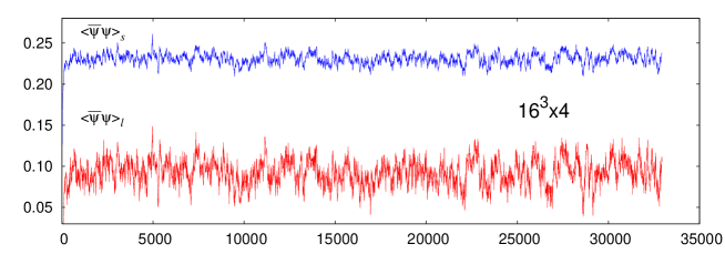
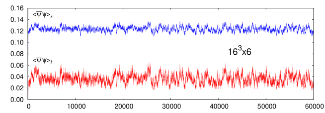
Figure 1: Time history of the light and strange quark chiral condensates for the smallest quark masses used in our simulations on lattices of temporal extent $N_{\tau}=4$ and $6$ and for values of the gauge coupling in the vicinity of the critical coupling of the transition on these lattices. The upper figure shows a run at $\beta=3.305$ with $\hat{m}_{l}=0.05\hat{m}_{s}$ on a $16^{3}\times 4$ lattice and the lower figure is for $\beta=3.46$ and $\hat{m}_{l}=0.1\hat{m}_{s}$ on a $16^{3}\times 6$ lattice.

In Figure 2(left) we compare results for the light quark chiral condensate calculated on lattices of size $8^{3}\times 4$ and $16^{3}\times 4$. It clearly reflects the presence of finite volume effects at small values of the quark mass. While finite volume effects seem to be negligible for $\hat{m}_{l}/\hat{m}_{s}\geq 0.2$, for $\hat{m}_{l}/\hat{m}_{s}=0.1$ we observe a small but statistically significant volume dependence for the chiral condensate as well as for the Polyakov loop expectation value. This volume dependence is even more pronounced for $\hat{m}_{l}/\hat{m}_{s}=0.05$ and seems to be stronger at low temperatures. While the value of the chiral condensate increases with increasing volume the Polyakov loop expectation value decreases (Figure 2(right)).

In a theory with Goldstone bosons, e.g. in $O(N)$-symmetric spin models, it is expected that in the broken phase the order parameter, ${\cal O}$, changes with the symmetry breaking field, $h$, as ${\cal O}(h)-{\cal O}(0)\sim h^{1/2}$ wallace . This behavior has also been found in QCD with adjoint quarks, i.e. $\langle\bar{\psi}\psi\rangle\sim c_{0}\;+\;c_{1}(m_{l}/T)^{1/2}$ lutgemeier ; engels . Our current analysis of the quark mass dependence of the chiral condensate is not yet accurate enough and has not yet been performed at small enough quark masses to verify this behavior explicitly. We will analyze the light quark mass limit in more detail elsewhere.

Figure 2: The light quark chiral condensate in units of $a^{-3}$ (left) and the Polyakov loop expectation value (right) as function of the bare light quark mass in units of the temperature, $m_{l}/T\equiv\hat{m}_{l}N_{\tau}$ for fixed $\beta$ and $\hat{m}_{s}=0.065$ on lattices of size $8^{3}\times 4$ (circle) and $16^{3}\times 4$ (triangles). Shown are results for various values of $\beta$ ranging from $\beta=3.28$ to $\beta=3.4$ (top to bottom for $\langle\bar{\psi}\psi\rangle$ and bottom to top for $\langle L\rangle$). Full and open symbols show results obtained from direct simulations and Ferrenberg-Swendsen interpolations, respectively.

We use the Polyakov loop susceptibility as well as the disconnected part of the chiral susceptibility to locate the transition temperature to the high temperature phase of QCD,

$$\chi_{L} \equiv N_{\sigma}^{3}\left(\langle L^{2}\rangle-\langle L\rangle^{2}\right)\;,$$ (4)

$$\frac{\chi_{q}}{T^{2}} \equiv \frac{N_{\tau}}{16N_{\sigma}^{3}}\left(\left\langle\left({\rm Tr}\;D^{-1}(\hat{m}_{q})\right)^{2}\right\rangle-\left\langle{\rm Tr\;}D^{-1}(\hat{m}_{q})\right\rangle^{2}\right)\;,\;q\;\equiv\;l,\;s.$$ (5)

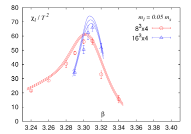
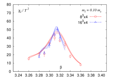
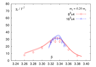
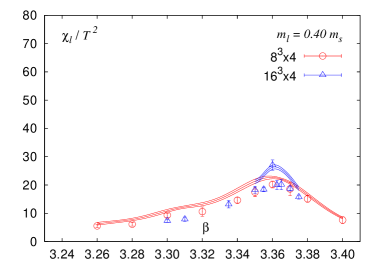
Figure 3: The disconnected part of the light quark chiral susceptibility on lattices of size $8^{3}\times 4$ (squares) and $16^{3}\times 4$ (circles) for four different values of the light quark mass. The curves show Ferrenberg-Swendsen interpolations of the data points obtained from multi-parameter histograms with an error band coming from Ferrenberg-Swendsen reweightings performed on different jackknife samples.

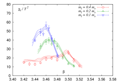
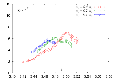
Figure 4: The disconnected part of the light quark chiral susceptibility (left) and the Polyakov loop susceptibility (right) on lattices of size $16^{3}\times 6$ for three different values of the light quark mass. Curves show Ferrenberg-Swendsen interpolations as discussed in the caption of Fig. 2

In Figure 3 we show results for the disconnected part of the light quark chiral susceptibility, $\chi_{l}$, calculated on $8^{3}\times 4$ and $16^{3}\times 4$ lattices. Results for $\chi_{l}$ and the Polyakov loop susceptibility, $\chi_{L}$, obtained from our calculations on $16^{3}\times 6$ lattices are shown in Figure 4. The location of peaks in the susceptibilities has been determined from a Ferrenberg-Swendsen reweighting of data in the vicinity of the peaks. Errors on the critical couplings determined in this way have been obtained from a jackknife analysis where Ferrenberg-Swendsen interpolations have been performed on different sub-samples. In agreement with earlier calculations we find that the position of peaks in $\chi_{l}$ and $\chi_{L}$ show only little volume dependence and that the peak height changes only little, although the maxima become somewhat more pronounced on the larger lattices. This is consistent with the transition being a crossover rather than a true phase transition in the infinite volume limit.

Although differences in the critical coupling extracted from $\chi_{L}$ and $\chi_{l}$ are small we find that on small lattices the peak in the Polyakov loop susceptibility is located at a systematically larger value of the gauge coupling $\beta$. In a finite volume this is, of course, not unexpected, and in the infinite volume limit an ambiguity in identifying the transition point may also remain for a crossover transition. Nonetheless, we observe that the difference $\beta_{c,L}-\beta_{c,l}$ decreases with increasing volume and is within errors consistent with zero for $16^{3}\times 4$, which has the largest spatial volume expressed in units of the temperature, $TV^{1/3}=4$. On the smallest lattice, $8^{3}\times 4$, we find $\beta_{c,L}-\beta_{c,l}\simeq 0.0077(9)$. Within the statistical accuracy of our data we also do not find any systematic quark mass dependence of this difference, $\beta_{c,L}-\beta_{c,l}$, which is shown in Figure 5 for the 3 different system sizes used in our calculations.

Figure 5: The difference of gauge couplings at the location of peaks in the Polyakov loop and chiral susceptibilities, $\beta_{c,L}-\beta_{c,l}$. Shown are results from calculations on $8^{3}\times 4$ (left), $16^{3}\times 4$ (middle) and $16^{3}\times 6$ (right).

The peak positions, $\beta_{c}(\hat{m}_{l},\hat{m}_{s},N_{\tau})$, in the chiral and Polyakov loop susceptibilities are generally well determined. An exception is our data set for $\hat{m}_{l}/\hat{m}_{s}=0.2$ on the $16^{3}\times 6$ lattice which shows a quite broad peak in $\chi_{l}$. Consequently we find here the largest difference $\beta_{c,L}-\beta_{c,l}\simeq 0.019(7)$ which also has the largest statistical error.

The error on $\beta_{c,(L,l)}(\hat{m}_{l},\hat{m}_{s},N_{\tau})$ translates, of course, into an uncertainty for the lattice spacing $a(\beta_{c})$ which in turn contributes to the error on the transition temperature. In order to get a feeling for the accuracy required in the determination of $\beta_{c}$ we give here an estimate for the dependence of the lattice cut-off on the gauge coupling, which will be determined and discussed in more detail in the next section. From an analysis of scales related to the static quark potential at zero temperature we deduce that, in the regime of couplings relevant for our finite temperature calculations, a shift in the gauge coupling by $\Delta\beta=0.02$ corresponds to a change in the lattice cut-off of about 5%. An uncertainty in the determination of the critical coupling of about $0.01$ thus translates into a 2.5% error on $T_{c}$.

We summarize our results for the critical couplings determined from peaks in $\chi_{L}$ and $\chi_{l}$, respectively, in Table 2. As the peak positions in both quantities apparently differ systematically on finite lattices and for finite values of the quark mass, we use the average of both values as an estimate for the critical coupling, $\beta_{c}$, for the transition to the high temperature phase of QCD. We include the deviation of $\beta_{c,L}$ and $\beta_{c,l}$ from this average value as a systematic error in $\beta_{c}$ and add it quadratically to the statistical error. These averaged critical couplings are given in the last column of Table 2. Even with this conservative error estimate the uncertainty in the determination of the critical coupling is in almost all cases smaller than $0.01$, i.e. the uncertainty in the determination of $\beta_{c}$ will amount to about 2% error in the determination of $T_{c}$.

$N_{\tau}$	$\hat{m}_{s}$	$~{}~{}\hat{m}_{l}$	$N_{\sigma}$	$\beta_{c,L}$ [from $\chi_{L}$]	$\beta_{c,l}$ [from $\chi_{l}$]	$\beta_{c,s}$ [from $\chi_{s}$]	$\beta_{c}$ [averaged]
4	0.1	0.05000	8	3.4248(46)	3.4125(32)	3.4132(36)	3.4187( 83)
		0.02000	8	3.3740( 31)	3.3676( 18)	3.3723( 35)	3.3708( 48)
4	0.065	0.02600	16	3.3637(20)	3.3618(12)	3.3615(13)	3.3627( 25)
		0.02600	8	3.3661(25)	3.3563(21)	3.3588(28)	3.3612( 59)
		0.01300	16	3.3389(18)	3.3362(17)	3.3374(17)	3.3376( 28)
		0.01300	8	3.3419(23)	3.3349(21)	3.3398(31)	3.3384( 47)
		0.00650	16	3.3140( 5)	3.3145( 3)	3.3132( 4)	3.3143(  6)
		0.00650	8	3.3239(30)	3.3141(11)	3.3198(24)	3.3190( 58)
		0.00325	16	3.3042(43)	3.3085(26)	3.3132(69)	3.3064( 55)
		0.00325	8	3.3087(18)	3.3024(10)	3.3047(17)	3.3056( 37)
6	0.04	0.01600	16	3.5002(25)	3.4973(12)	3.4967(12)	3.4988( 32)
		0.00800	16	3.4801(19)	3.4595(19)	3.4614(44)	3.4698(106)
		0.00400	16	3.4668(24)	3.4604(18)	3.4603(11)	3.4636( 44)

Table 2: Critical couplings determined from the location of peaks in the Polyakov loop susceptibility as well as in the disconnected parts of the light and strange quark chiral susceptibilities. The last column gives the average of $\beta_{c,L}$ and $\beta_{c,l}$.

In addition to the light quark condensate and its susceptibility we also have analyzed the strange quark condensate and its susceptibility, $\chi_{s}$. We find that the light and heavy quark condensates are strongly correlated, which is easily seen in the MD-time evolution of these quantities. Already on the smallest lattices the position of the peak in the heavy quark susceptibilities is consistent with that deduced from the light quark condensate. On the larger, $N_{\sigma}=16$, lattices the difference $|\beta_{c,l}-\beta_{c,s}|$ is in all cases zero within statistical errors, which are about $3\cdot 10^{-3}$. Any temperature difference in the crossover behavior for the light and strange quark sector of QCD, which sometimes is discussed in phenomenological models, thus is below the $1$ MeV level.

IV Zero Temperature Scales

In order to calculate the transition temperature in terms of an observable that is experimentally accessible and can be used to set the scale for $T_{c}$ we have to perform a zero temperature calculation at the critical couplings $\beta_{c}$ determined in the previous section. This will allow us to eliminate the unknown lattice cut-off, $a(\beta_{c})$, which determines $T_{c}$ on a lattice with temporal extent $N_{\tau}$, i.e. $T_{c}=1/N_{\tau}a(\beta_{c})$. To do so we have performed calculations at zero temperature, i.e. on lattices of size $16^{3}\times 32$, and calculated several hadron masses as well as the static quark potential. From the latter we determine the string tension and extract short distance scale parameters $r_{0},~{}r_{1}$, which are defined as separations between the static quark anti-quark sources at which the force between them attains certain values Sommer ,

$$r^{2}\frac{{\rm d}V_{\bar{q}q}(r)}{{\rm d}r}\biggl{|}_{r=r_{0}}=1.65\;\;,\;\;r^{2}\frac{{\rm d}V_{\bar{q}q}(r)}{{\rm d}r}\biggl{|}_{r=r_{1}}=1.0\;.$$ (6)

Although these scale parameters are not directly accessible to experiment they can be well estimated from heavy quarkonium phenomenology. Moreover, they have been determined quite accurately in lattice calculations through a combined analysis of the static quark potential MILCpotential and level splittings in bottomonium spectra gray . Both these calculations have been performed on identical sets of gauge field configurations. We will use the value for $r_{0}$ determined in the bottomonium calculation gray for all conversions of lattice results to physical units,

$$r_{0}=0.469(7)\;{\rm fm}\;.$$ (7)

Our zero temperature calculations have been performed at values of the gauge coupling in the vicinity of the $\beta_{c}$ values listed in the last column of Table 2. We typically generated several thousand configurations and analyzed the hadron spectrum and static quark potential on every $10^{th}$ configuration. A summary of our zero temperature simulation parameters is given in Table 3 together with the two scales characterizing the static quark potential, $r_{0}/a$ and $\sqrt{\sigma}a$, expressed in lattice units. These scales have been obtained by using the simple Cornell form to fit our numerical results for the static quark potential, $V_{\bar{q}q}(r)=-\alpha/r+\sigma r+c$. With this fit-ansatz, which does not include a possible running of the coupling $\alpha$, the force entering the definition of $r_{0}$ is easily calculated and we find from Eq. 6, $r_{0}\equiv\sqrt{(1.65-\alpha)/\sigma}$. More details on the analysis of the static quark potential and the precise form for the fit ansatz used by us will be given in the next subsection.

In addition we also have calculated some meson masses, the mass of the lightest pseudo-scalar in the light quark sector, $m_{ps}$ and the strange quark sector, $m_{s\bar{s}}$; and the pseudo-scalar heavy-light meson, $m_{K}$. Results for these masses are also given in Table 3. They have been obtained from point-wall correlation functions using a $Z_{2}$-wall source. The correlation functions have been fitted to a double exponential ansatz that takes into account the two lowest states contributing to the staggered fermion correlation functions. We have varied the lower limit, $r_{min}$, of the fit range to check for the stability of our fits. For the masses displayed in Table 3 stable results typically are found for $r_{min}\raise 1.29167pt\hbox{$>$\kern-7.5pt\raise-4.73611pt\hbox{$\sim$}}6$ for $N_{\tau}=4$ and $r_{min}\raise 1.29167pt\hbox{$>$\kern-7.5pt\raise-4.73611pt\hbox{$\sim$}}8$ for $N_{\tau}=6$. In the following we discuss in more detail our analysis of the static quark potential.

$\hat{m}_{s}$	$~{}~{}\hat{m}_{l}$	$~{}~{}\beta$	# conf.	$m_{ps}a$	$m_{s\bar{s}}a$	$m_{K}a$	$r_{0}/a$	$(r_{0}/a)_{smooth}$	$\sqrt{\sigma}a$
0.1	0.05	3.409	600	0.7075(3)	0.9817(2)	0.8571(3)	2.0525(36)(89)	-	0.5564(17)(79)
	0.02	3.371	560	0.4583(2)	0.9854(4)	0.7748(3)	2.0178(45)(56)	2.0097	0.5651(24)(92)
0.065	0.026	3.362	500	0.5202(4)	0.8045(3)	0.6794(6)	2.0250(59)(75)	2.0337	0.5580(26)(89)
	0.013	3.335	400	0.3733(3)	0.8072(4)	0.6339(4)	1.9801(47)(11)	1.9803	0.5675(24)(90)
	0.0065	3.31	750	0.2656(4)	0.8089(2)	0.6092(5)	1.9047(40)(132)	1.9018	0.5910(25)(116)
	0.00325	3.30	400	0.1888(6)	0.8099(3)	0.5948(3)	1.8915(59)(136)	1.8750	0.5888(34)(95)
0.04	0.016	3.50	294	0.3864(6)	0.5988(6)	0.5048(6)	3.0061(143)(92)	3.0136	0.3766(27)(33)
	0.008	3.47	500	0.2831(13)	0.6097(6)	0.4789(7)	2.8953(96)(56)	2.8736	0.3867(19)(40)
	0.004	3.455	410	0.2043(10)	0.6143(6)	0.4634(7)	2.8030(75)(51)	2.8056	0.4016(19)(43)

Table 3: Simulation parameter for the scale setting runs on $16^{3}\times 32$ lattices and results obtained for light and heavy quark pseudo-scalars ($m_{ps}$ and $m_{s\bar{s}}$), the kaon mass and scale parameters of the heavy quark potential. In column 4 we give the number of configurations actually used in the analysis. Column 9 show the smoothed values for $r_{0}/a$ obtained from the fit ansatz given in Eq.12. Results for the largest quark mass pair, $(\hat{m}_{s},\hat{m}_{l})=(0.1,0.05)$, have not been included in the fit.

IV.1 The static quark potential

The static quark potential at fixed spatial separation has been obtained from an extrapolation of ratios of Wilson loops to infinite time separation. The spatial transporters in the Wilson loop were constructed from spatially smeared links which have been obtained iteratively by adding space-like 3-link staples with a relative weight $\gamma=0.4$ to the links and projecting this sum back to an element of the $SU(3)$ gauge group (APE smearing). This process has been repeated 10 times. We have calculated the potential for on-axis as well as off-axis spatial separations. As we have to work on still rather coarse lattices and need to know the static quark potential at rather short distances (in lattice units) we have to deal with violations of rotational symmetry in the potential. In our analysis of the potential we take care of this by adopting a strategy used successfully in the analysis of static quark potentials Sommer and heavy quark free energies zantow . We replace the Euclidean distance on the lattice, $(r/a)^{2}=n_{x}^{2}+n_{y}^{2}+n_{z}^{2}$, by $r_{I}/a$ which relates the separation between the static quark and anti-quark sources to the Fourier transform of the tree-level lattice gluon propagator, $D_{\mu\nu}$, i.e.

$$(r_{I}/a)^{-1}=4\pi\int_{-\pi}^{\pi}\frac{d^{3}k}{{(2\pi)}^{3}}\exp(i\vec{k}\cdot\vec{n})D_{00}(k)\quad.$$ (8)

which defines the lattice Coulomb potential. Here the integers $n=(n_{x},n_{y},n_{z})$ label the spatial components of the 4-vector for all lattice sites and $D_{00}$ is the time-like component of $D_{\mu\nu}$. For the ${\cal O}(a^{2})$ improved gauge action used here this is given by

$$D^{-1}_{00}(k)=4\sum_{i=1}^{3}\left(\sin^{2}\frac{k_{i}}{2}+\frac{1}{3}\sin^{4}\frac{k_{i}}{2}\right)\quad.$$ (9)

This procedure removes most of the short distance lattice artifacts. It allows us to perform fits to the heavy quark potential with the 3-parameter ansatz,

$$V_{\bar{q}q}(r)=-\frac{\alpha}{r_{I}}+\sigma r_{I}+c\;.$$ (10)

Fit results for $\sqrt{\sigma}a$ and $r_{0}/a=\sqrt{(1.65-\alpha)/\sigma a^{2}}$ obtained with this ansatz are given in Table 3. Errors on both quantities have been calculated from a jackknife analysis. We also performed fits with a 4-parameter ansatz commonly used in the literature,

$$V_{\bar{q}q}(r)=-\frac{\alpha}{r}+\sigma r+\alpha^{\prime}\left(\frac{1}{r_{I}}-\frac{1}{r}\right)+c\;.$$ (11)

Using this ansatz for our fits, we generally obtain results which are compatible with the fit parameters extracted from the 3-parameter fit. We combine the difference between the 4-parameter fit result and the 3-parameter fit with differences that arise when changing the fit range for the potentials and quote this as a systematic error. This is given as a second error for $r_{0}/a$ and $\sqrt{\sigma}a$ listed in Table 3. Using Eq. 7 we find that the lattice spacings corresponding to the relevant coupling range explored in our $N_{\tau}=4$ and $6$ calculations correspond to $a\simeq 0.24$ fm and $a\simeq 0.17$ fm, respectively. As can be seen from Table 3 we obtain values for $r_{0}\sqrt{\sigma}$ between $1.11$ and $1.13$. These values are about 2% larger than those obtained on finer lattices by the MILC collaboration MILCpotential .

We have determined the scale parameter $r_{0}$ in units of the lattice spacing for 9 different parameter sets $(\hat{m}_{l},\hat{m}_{s},\beta)$. This allows to interpolate between different values of the gauge coupling and quark masses. We use a renormalization group inspired ansatz allton which takes into account the quark mass dependence of $r_{0}/a$ Bernard04 and which approaches, in the weak coupling limit, the 2-loop $\beta$-function for three massless flavors,

$$(r_{0}/a)^{-1}=R(\beta)(1+B\hat{a}^{2}(\beta)+C\hat{a}^{4}(\beta)){\rm e}^{A(2\hat{m}_{l}+\hat{m}_{s})+D}\;.$$ (12)

Here $R(\beta)$ denotes the 2-loop $\beta$-function and $\hat{a}(\beta)=R(\beta)/R(\bar{\beta})$ with $\bar{\beta}=3.4$ chosen as an arbitrary normalization point. A fit to 14 values for $r_{0}/a$, which include 8 of the 9 values for $r_{0}/a$ given in Table 3 and additional data obtained in our studies of 3-flavor QCD RHMCtuning , gives $A=1.45(5)$, $B=1.20(17)$, $C=-0.21(6)$ and $D=2.41(5)$ with a $\chi^{2}/dof=0.9$. We use this interpolation formula to set the scale for the transition temperature.

IV.2 The physical point

Our goal is to determine the transition temperature at the physical point, i.e. for quark masses that correspond to the physical light and strange quark masses that reproduce the experimentally known hadron mass spectrum at zero temperature. To do so we reduce the bare light quark mass, $\hat{m}_{l}$, keeping $\hat{m}_{s}$ fixed to an appropriate value that yields the physical value for the pion mass expressed, for instance, in units of $r_{0}$, i.e. $m_{ps}r_{0}=0.321(5)$. The strange quark mass should also be chosen such that, at this point, one of the strange meson masses is reproduced. For this purpose we monitor the value of the kaon mass and the strange pseudo-scalar, $m_{s\bar{s}}$. In the continuum limit the physical point is then given as $(m_{ps}r_{0},m_{K}r_{0})=(0.321(5),1.177(18))$ where the error reflects the uncertainty in $r_{0}$ gray . At this point the strange pseudo-scalar in units of $r_{0}$ is given by $m_{s\bar{s}}r_{0}=1.631(24)$.

In Figure 6, we show the kaon masses in units of $r_{0}$, corresponding to the different sets of light and heavy quark mass values used in our calculations, plotted versus pseudo-scalar masses in units of $r_{0}$. These data are also given in Table 3. It can be seen that the two bare strange quark mass values, $\hat{m}_{s}=0.065$ and $0.04$, used in our finite temperature calculations on $N_{\tau}=4$ and $6$ lattices, respectively, allow us to approach the physical point in the light quark mass limit. For $m_{ps}r_{0}=0.321$ we obtain $m_{K}r_{0}=1.12$ and $1.25$ for the two parameter sets, which agrees with the continuum value for the kaon mass within 6%. The strange pseudo-scalar mass is, as expected, almost independent of the value of the light quark mass. Using the data displayed in Table 3 we find from a linear extrapolation to the physical point, $m_{s\bar{s}}r_{0}=1.53(2)$ ($\hat{m}_{s}=0.065$ data set) and $m_{s\bar{s}}r_{0}=1.69(2)$ ($\hat{m}_{s}=0.04$ data set), respectively. This too agrees with the continuum value within 6%.

For the third parameter set, $\hat{m}_{s}=0.1$, we obtain extrapolated values for the kaon mass, $m_{K}r_{0}=1.41$ and for the strange pseudo-scalar $m_{s\bar{s}}r_{0}=1.96$, which both are about 20% larger than the physical values. We use this parameter set to verify the insensitivity of $T_{c}r_{0}$ to the precise choice of the strange quark mass.

Figure 6: The square of the kaon mass in units of $r_{0}^{2}$ versus the square of the pseudo-scalar meson mass also expressed in units of $r_{0}^{2}$. Shown are results for the three different sets of bare strange quark masses, $\hat{m}_{s}=0.04$, (squares) $0.065$ (circles) and $0.1$ (triangles). The star shows the location of the physical point using $r_{0}=0.469$ fm. The values of the light quark masses and gauge couplings at which the zero temperature calculations on $16^{3}\times 32$ lattice have been performed can be found in Table 3.

V The transition temperature

To obtain the transition temperature we use the results for the scales $r_{0}/a$ and $\sqrt{\sigma}a$ obtained from fits to the static quark potential. In cases where zero temperature calculations have not been performed directly at the critical coupling but at a nearby $\beta$-value we use Eq. 12 to determine the scales at $\beta_{c}(\hat{m}_{l},\hat{m}_{s},N_{\tau})$. The transition temperature is then obtained as $T_{c}r_{0}\equiv(r_{0}/a)/N_{\tau}$ or $T_{c}/\sqrt{\sigma}=1/\sqrt{\sigma}aN_{\tau}$. We show these results as function of the pseudo-scalar (pion) mass expressed in units of $r_{0}$ in Figure 7. There we give 2 errors on $T_{c}r_{0}$ and $T_{c}/\sqrt{\sigma}$. A thin error bar reflects the combined statistical and systematic errors on the scales $r_{0}/a$ and $\sqrt{\sigma}a$ obtained from our 3-parameter fit to the static quark potential. The broad error bar combines this uncertainty of the zero temperature scale determination with the scale-uncertainty arising from the error on $\beta_{c}$. As can be seen, the former error, which typically is of the order of 2%, dominates our uncertainty on $T_{c}r_{0}$ and $T_{c}/\sqrt{\sigma}$ on the coarser $N_{\tau}=4$ lattices, while the uncertainty in the determination of $\beta_{c}$ becomes more relevant for $N_{\tau}=6$. Values for the transition temperatures are given in Table 4.

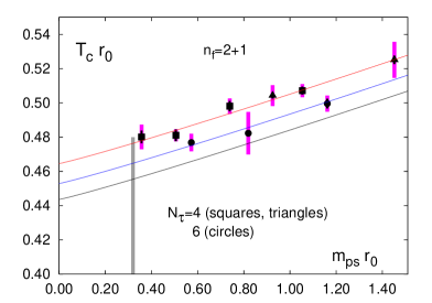
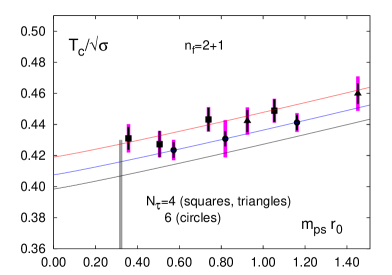
Figure 7: $T_{c}r_{0}$ (left) and $T_{c}/\sqrt{\sigma}$ (right) as a function of $m_{ps}r_{0}$ on lattices with temporal extent $N_{\tau}=4$, $\hat{m}_{s}=0.065$ (squares) and $\hat{m}_{s}=0.1$ (triangles) as well as for $N_{\tau}=6$, $\hat{m}_{s}=0.04$ (circles). Thin error bars represent the statistical and systematic error on $r_{0}/a$ and $\sqrt{\sigma}a$. The broad error bar combines this error with the error on $\beta_{c}$. The vertical line shows the location of the physical value $m_{ps}r_{0}=0.321(5)$ and its width represents the error on $r_{0}$. The three parallel lines show results of fits based on Eq. 13 with $d=1.08$ for $N_{\tau}=4,~{}6$ and $N_{\tau}\rightarrow\infty$ (top to bottom).

$N_{\tau}$	$\hat{m}_{s}$	$~{}~{}\hat{m}_{l}$	$T_{c}r_{0}$	$T_{c}/\sqrt{\sigma}$
4	0.1	0.02	0.5043( 61)	0.4422( 88)
		0.05	0.5251(105)	0.4598(111)
4	0.065	0.00325	0.4801( 72)	0.4311( 91)
		0.0065	0.4811( 35)	0.4273( 84)
		0.013	0.4981( 45)	0.4432( 79)
		0.026	0.5071( 38)	0.4488( 77)
6	0.04	0.004	0.4768( 51)	0.4236( 66)
		0.008	0.4823(124)	0.4308(120)
		0.016	0.4996( 47)	0.4413( 61)

Table 4: Transition temperature in units of $r_{0}$ and $\sqrt{\sigma}$. The errors given are the combined statistical errors discussed in the text.

The comparison of results obtained on lattices with temporal extent $N_{\tau}=4$ and $6$ given in Figure 7 clearly shows a systematic cut-off dependence for the transition temperature. At fixed values of $m_{ps}r_{0}$, results obtained for $N_{\tau}=6$ are systematically smaller than the $N_{\tau}=4$ results by about (3-4)%. On the other hand, we see no statistically significant dependence of our results on the value of the strange quark mass; results obtained on the $N_{\tau}=4$ lattice with a strange quark mass $\hat{m}_{s}=0.1$ and $\hat{m}_{s}=0.065$ are in good agreement. The former choice of parameters leads to a kaon mass that is about 20% larger than in the latter case.

We have extrapolated our numerical results for $T_{c}r_{0}$ and $T_{c}/\sqrt{\sigma}$, which have been obtained for a specific set of lattice parameters ($\hat{m}_{l},\hat{m}_{s},N_{\tau}$), to the chiral and continuum limit using an ansatz that takes into account the quadratic cut-off dependence, $(aT)^{2}=1/N_{\tau}^{2}$, and a quark mass dependence expressed in terms of the pseudo-scalar meson mass,

$$Y_{\hat{m}_{l},\hat{m}_{s},N_{\tau}}=Y_{0,m_{s},\infty}+A(m_{ps}r_{0})^{d}+B/N_{\tau}^{2}\quad,\quad Y=T_{c}r_{0},~{}T_{c}/\sqrt{\sigma}\;,$$ (13)

If the QCD transition is second order in the chiral limit the transition temperature is expected to depend on the quark mass as $\hat{m}_{l}^{1/\beta\delta}$, or correspondingly on the pseudo-scalar meson mass as $m_{ps}^{2/\beta\delta}$ with $d\equiv 2/\beta\delta\simeq 1.08$ characterizing universal scaling behavior in the vicinity of second order phase transitions belonging to the universality class of $O(4)$ symmetric, 3-dimensional spin models. If, however, the transition becomes first order for small quark masses, which is not ruled out for physical values of the strange quark mass, the transition temperature will depend linearly on the quark mass ($d=2$). A fit to our data set with $d$ as a free fit parameter would actually favor a value smaller than unity, although the error on $d$ is large in this case, $d=0.6(7)$.

Fortunately, the extrapolation to the physical point is not very sensitive to the choice of $d$ as our calculations have been performed close to this point. It does, however, increase the uncertainty on the extrapolation to the chiral limit. We have performed extrapolations to the chiral limit with $d$ varying between $d=1$ and $d=2$. From this we find

$$m_{ps}r_{0}\equiv 0:\qquad T_{c}r_{0}=0.444(6)^{+12}_{-3}\quad,\quad T_{c}/\sqrt{\sigma}=0.398(6)^{+10}_{-1}\;,$$ (14)

where the central value is given for fits with the $O(4)$ exponent $d=1.08$ and the lower and upper systematic error correspond to $d=1$ and $d=2$, respectively. Using the fit values for the parameter $A$ that controls the quark mass dependence of $T_{c}r_{0}$ ($A=0.041(5)$) and $T_{c}/\sqrt{\sigma}$ ($A=0.029(4)$), respectively, we can determine the transition temperature at the physical point, fixed by $m_{ps}r_{0}$r, where we then obtain a slightly larger value with reduced systematic errors,

$$m_{ps}r_{0}\equiv 0.321(5):\qquad T_{c}r_{0}=0.457(7)^{+8}_{-2}\quad,\quad T_{c}/\sqrt{\sigma}=0.408(8)^{+3}_{-1}\;.$$ (15)

Here the error includes the uncertainty in the value for the physical point, $m_{ps}r_{0}$, arising from the uncertainty in the scale parameter $r_{0}=0.469(7)$ fm. We note that the extrapolated values for $T_{c}r_{0}$ and $T_{c}/\sqrt{\sigma}$ may also be interpreted as a continuum extrapolation of the shape parameters of the static potential. This yields $r_{0}\sqrt{\sigma}\simeq 1.11$ which is consistent with the continuum extrapolation obtained with the asqtad-action Bernard04 .

The fit parameter $B$ which controls the size of the cut-off dependent term in Eq. 13 is in all cases close to $1/3$. We find $B=0.34(9)$ for fits to $T_{c}r_{0}$ and $B=0.33(7)$ for fits to $T_{c}/\sqrt{\sigma}$, respectively. The critical temperatures for $N_{\tau}=4$ thus are about 5% larger than the extrapolated value, and for $N_{\tau}=6$ the difference is about 2%. We therefore expect that any remaining uncertainties in our extrapolation to the continuum limit which may arise from higher order corrections in the cut-off dependence of $T_{c}r_{0}$ are not larger than 2%.

The results for the transition temperature obtained here for smaller quark masses and smaller lattice spacings is entirely consistent with the results for 2-flavor QCD obtained previously with the p4fat3 action on $N_{\tau}=4$ lattices in the chiral limit, $T_{c}/\sqrt{\sigma}=0.425(15)$ peikert . We now find for (2+1)-flavor QCD for $N_{\tau}=4$ in the chiral limit $T_{c}/\sqrt{\sigma}=0.419(6)$. The continuum extrapolated result is, however, somewhat larger than the continuum extrapolated result obtained with the asqtad-action for (2+1)-flavor QCD in the chiral limit, $T_{c}r_{0}=0.402(29)$ Bernard04 , which is based on the determination of transition temperatures on lattices with temporal extent $N_{\tau}=4$, $6$ and $8$.

V.1 Using zero temperature scales to convert $T_{c}$ to physical units

Although we frequently have referred to the physical value of $r_{0}$ during the discussion in the previous chapters we stress that our final result for dimensionless quantities, in particular $T_{c}r_{0}$ and $T_{c}/\sqrt{\sigma}$ given in Eq. 14, does not depend on the actual physical value of $r_{0}$ or $\sqrt{\sigma}$.

As pointed out in the previous section, the results obtained here for $T_{c}$ expressed in units of $r_{0}$ or $\sqrt{\sigma}$ are consistent with earlier determinations of these quantities. In fact, after extrapolation to the continuum limit this ratio turns out to be even somewhat smaller than those determined previously for $2$-flavor QCD.

Unfortunately neither $r_{0}$ nor $\sqrt{\sigma}$ are directly measurable experimentally. Their physical values have been deduced from lattice calculations through a comparison with calculations for the level splitting in the bottomonium spectrum gray ; Bernard04 . This observable has the advantage of showing only a weak quark mass dependence. Of course, dealing with heavy quarks in addition to the dynamical light quarks requires a special set-up (NRQCD) which might introduce additional systematic errors. However, these findings have been cross-checked through calculations of other observables which only involve the light quark sector. In particular, the pion decay constant, $f_{\pi}$, has been evaluated on the MILC configurations that have been used for the bottomonium level splitting and yields a consistent value for $r_{0}$ Davies . One may, of course, also consider using results for masses of mesons constructed from light quarks, e.g. the vector meson mass, to determine the scale for the transition temperature, eg. $T_{c}/m_{\rho}$. However, even on lattices with smaller lattice spacings than those used in thermodynamic calculations today, the calculation of vector meson mass is known to suffer from large statistical and systematic errors MILCpotential ; Davies . This is even more the case on the coarse lattices needed for our finite temperature calculations. We thus refrained from using results on the vector meson mass for our determination of the transition temperature.

At present the scale parameter $r_{0}$, deduced from the bottomonium level splitting using NRQCD gray , seems to be the best controlled lattice observable that can be used to set the scale for $T_{c}$. Using for $r_{0}$ the value given in Eq. 7 we obtain for the transition temperature in QCD at the physical point,

$$T_{c}=192(7)(4)\;{\rm MeV}\;,$$ (16)

where the statistical error includes the errors given in Eq. 15 as well as the uncertainty in the value of $r_{0}$ and the second error reflects our estimate of a remaining systematic error on the extrapolation to the continuum limit. As discussed after Eq. 15 we estimate this error which arises from neglecting higher order cut-off effects in our ansatz for the continuum extrapolation, Eq. 13 to be about 2%.

The value of the critical temperature obtained here is about 10% larger than the frequently quoted value $\sim 175$ MeV. We note that this larger value mainly results from the value for $r_{0}$ used in our conversion to physical scales. Together with $r_{0}\sqrt{\sigma}\simeq 1.11$ it implies that the string tension takes on the value $\sqrt{\sigma}\simeq 465$ MeV. This value of the string tension is about 10% larger than that used in the past to set the scale for $T_{c}$ peikert .

VI Conclusions

We have presented new results on the transition temperature in QCD with an almost physical quark mass spectrum. The extrapolation to the physical point and the continuum limit is based on numerical calculations with an improved staggered fermion action which have been performed on lattices with two different values of the lattice cut-off and seven different values of bare light and strange quark masses.

It previously has been observed that the QCD transition temperature is close to the freeze-out temperature extracted from observed particle yields in heavy ion experiments stachel ; cleymans . Recent results from the RHIC experiments determine this freeze-out temperature to be below $170$ MeV PHENIX ; STAR . Our results on the transition temperature now seem to suggest that an intermediate regime between the QCD transition and freeze-out exists during which the system created in a heavy ion collision persists in a dense hadronic phase.

The analysis presented here leads to a value for the critical temperature with about 5% statistical and systematic errors. It clearly is desirable to confirm our estimate of the remaining systematic errors through an additional calculation on an even finer lattice. Furthermore, it is desirable to verify this result through calculations that explore other discretization schemes for the fermion sector of QCD and to also obtain a reliable independent scale setting for the transition temperature from an observable not related to properties of the static quark potential.

Appendix: Summary of simulation parameters and results

In this Appendix we summarize all numerical results from our simulations with two light and a heavier strange quark mass. The header line for all tables display the temporal lattice size $N_{\tau}$ and values of the light ($\hat{m}_{l}$) and strange ($\hat{m}_{s}$) quark masses. The first 4 columns of the Tables display the spatial lattice size, $N_{\sigma}$, the value of the gauge coupling, $\beta$, the number of configurations and the auto-correlation time in units of gauge field configurations generated at the end of a Molecular Dynamics trajectory of length $\tau_{MD}=0.5$. The next three columns give the Polyakov loop expectation value and the light and strange quark chiral condensates. The remaining three columns give the corresponding susceptibilities of these three observables. Note that on the $24^{3}\times 6$ lattice the strange quark condensate and its susceptibility have not been evaluated. We also do not quote a value for the light quark chiral susceptibility in this case, as the current statistics is not yet sufficient to determine this reliably. All data are given in units of appropriate powers of the lattice spacing.

$N_{\tau}=4,~{}~{}\hat{m}_{s}=0.065,~{}~{}\hat{m}_{l}=0.00325$
$N_{\sigma}$	$~{}~{}\beta$	# conf.	$\tau$	$\langle L\rangle$	$\langle\bar{\psi}\psi\rangle_{l}$	$\langle\bar{\psi}\psi\rangle_{s}$	$\chi_{L}$	$\chi_{l}$	$\chi_{s}$
8	3.2400	15500	32	0.0260( 6)	0.1854(17)	0.2908( 9)	0.086( 4)	1.34( 4)	0.235(13)
	3.2600	19000	40	0.0309(10)	0.1647(15)	0.2769( 8)	0.114( 6)	1.79( 7)	0.289(13)
	3.2800	30000	61	0.0374( 8)	0.1400(18)	0.2619( 9)	0.164( 7)	2.53(16)	0.477(41)
	3.2900	30000	89	0.0457(10)	0.1189(15)	0.2497( 8)	0.204(10)	3.01( 8)	0.519(25)
	3.3000	30000	81	0.0548(13)	0.0954(26)	0.2372(12)	0.257( 8)	3.50( 9)	0.631(23)
	3.3100	30000	84	0.0626(16)	0.0778(31)	0.2267(15)	0.284(15)	3.53(14)	0.698(36)
	3.3200	20000	57	0.0772(10)	0.0481(17)	0.2098( 9)	0.247(17)	2.06(19)	0.540(55)
	3.3400	20000	40	0.0902(12)	0.0297(15)	0.1939( 9)	0.241(17)	0.97(16)	0.414(32)
16	3.2900	38960	66	0.0424( 4)	0.1313( 5)	0.2513( 3)	0.221(10)	2.15(12)	0.510(28)
	3.3000	40570	101	0.0520( 6)	0.1084(10)	0.2389( 5)	0.279(11)	3.16(17)	0.645(37)
	3.3050	32950	105	0.0588( 7)	0.0927(13)	0.2309( 6)	0.314(22)	3.90(30)	0.743(58)
	3.3100	42300	102	0.0649( 5)	0.0791(11)	0.2240( 5)	0.314(11)	4.12(17)	0.778(34)
	3.3200	39050	92	0.0760( 4)	0.0544( 8)	0.2108( 4)	0.310(20)	3.22(21)	0.663(48)

Table A.1

$N_{\tau}=4,~{}~{}\hat{m}_{s}=0.065,~{}~{}\hat{m}_{l}=0.0065$
$N_{\sigma}$	$~{}~{}\beta$	# conf.	$\tau$	$\langle L\rangle$	$\langle\bar{\psi}\psi\rangle_{l}$	$\langle\bar{\psi}\psi\rangle_{s}$	$\chi_{L}$	$\chi_{l}$	$\chi_{s}$
8	3.2600	10000	37	0.0272( 7)	0.1868(12)	0.2828( 8)	0.097( 7)	0.95( 9)	0.289(34)
	3.2800	30000	45	0.0352( 8)	0.1604(12)	0.2646( 6)	0.149(12)	1.28(11)	0.363(32)
	3.2900	8900	56	0.0394(16)	0.1490(24)	0.2573(12)	0.146(17)	1.32(19)	0.334(53)
	3.3000	30000	76	0.0456( 9)	0.1314(13)	0.2465( 7)	0.207( 5)	2.11( 7)	0.565(20)
	3.3100	30000	105	0.0542(21)	0.1127(30)	0.2346(16)	0.269(18)	2.51(17)	0.649(54)
	3.3200	34380	191	0.0671(18)	0.0869(27)	0.2197(15)	0.280(12)	2.30( 9)	0.630(32)
	3.3300	30000	101	0.0780(17)	0.0665(25)	0.2067(14)	0.288(26)	1.99(24)	0.626(70)
	3.3400	20000	75	0.0884(18)	0.0506(23)	0.1957(16)	0.248(14)	1.13(11)	0.472(35)
	3.3600	12750	30	0.1017(25)	0.0344(14)	0.1798(16)	0.242(16)	0.50( 7)	0.361(29)
16	3.2800	20510	56	0.0312( 3)	0.1662( 3)	0.2664( 2)	0.168(10)	1.10( 9)	0.379(23)
	3.2900	30160	79	0.0380( 6)	0.1507( 8)	0.2562( 4)	0.212(16)	1.38(10)	0.432(29)
	3.3000	36100	76	0.0445( 3)	0.1351( 6)	0.2464( 3)	0.244(16)	1.96(15)	0.574(42)
	3.3100	40440	110	0.0542( 4)	0.1146( 5)	0.2343( 2)	0.316(14)	2.74(11)	0.740(34)
	3.3150	45570	141	0.0612( 6)	0.1007(10)	0.2262( 6)	0.334(15)	3.12(17)	0.820(44)
	3.3200	32310	81	0.0666( 7)	0.0896(10)	0.2198( 5)	0.304(17)	2.51(20)	0.647(51)

Table A.2

$N_{\tau}=4,~{}~{}\hat{m}_{s}=0.065,~{}~{}\hat{m}_{l}=0.013$
$N_{\sigma}$	$~{}~{}\beta$	# conf.	$\tau$	$\langle L\rangle$	$\langle\bar{\psi}\psi\rangle_{l}$	$\langle\bar{\psi}\psi\rangle_{s}$	$\chi_{L}$	$\chi_{l}$	$\chi_{s}$
8	3.2600	10000	26	0.0255( 9)	0.2075( 7)	0.2865( 6)	0.083( 7)	0.48( 3)	0.228( 9)
	3.2800	10000	45	0.0315( 9)	0.1865(19)	0.2705(14)	0.118( 8)	0.73( 7)	0.314(31)
	3.3000	20000	58	0.0383(13)	0.1645(20)	0.2545(13)	0.168(11)	1.13(11)	0.436(44)
	3.3200	30000	109	0.0520(18)	0.1372(22)	0.2355(14)	0.254(14)	1.64(10)	0.621(38)
	3.3300	30000	134	0.0621(18)	0.1188(22)	0.2231(14)	0.294(12)	1.68( 9)	0.620(38)
	3.3400	20000	79	0.0747(18)	0.0991(25)	0.2098(16)	0.303(15)	1.68( 9)	0.669(38)
	3.3600	17720	52	0.0948(17)	0.0695(19)	0.1879(13)	0.268(14)	0.96( 7)	0.473(21)
	3.3800	10000	40	0.1091(15)	0.0521(10)	0.1707( 8)	0.237(11)	0.41( 3)	0.296(20)
16	3.3200	20680	85	0.0501( 6)	0.1387( 8)	0.2356( 5)	0.293(24)	1.60(16)	0.612(66)
	3.3250	54840	114	0.0554( 6)	0.1295( 7)	0.2295( 4)	0.298(16)	1.82(14)	0.680(51)
	3.3300	50000	149	0.0615( 5)	0.1185( 7)	0.2222( 4)	0.340(13)	1.94( 8)	0.730(33)
	3.3350	55600	124	0.0673( 4)	0.1091( 6)	0.2160( 4)	0.330(17)	1.92(10)	0.711(37)
	3.3400	60000	104	0.0741( 6)	0.0980( 8)	0.2085( 5)	0.355(12)	1.95( 7)	0.733(26)
	3.3450	32560	82	0.0803( 5)	0.0886( 6)	0.2021( 4)	0.315(18)	1.61(13)	0.650(47)
	3.3500	20780	65	0.0859( 5)	0.0801( 6)	0.1960( 4)	0.303(20)	1.31(11)	0.572(46)

Table A.3

$N_{\tau}=4,~{}~{}\hat{m}_{s}=0.065,~{}~{}\hat{m}_{l}=0.026$
$N_{\sigma}$	$~{}~{}\beta$	# conf.	$\tau$	$\langle L\rangle$	$\langle\bar{\psi}\psi\rangle_{l}$	$\langle\bar{\psi}\psi\rangle_{s}$	$\chi_{L}$	$\chi_{l}$	$\chi_{s}$
8	3.2600	10000	30	0.0235( 6)	0.2378(14)	0.2918(10)	0.076( 5)	0.35( 4)	0.217(21)
	3.2800	10000	22	0.0270( 9)	0.2241( 8)	0.2802( 5)	0.096( 7)	0.38( 4)	0.226(20)
	3.3000	9530	39	0.0311(12)	0.2091(15)	0.2675(12)	0.134(10)	0.58( 5)	0.339(28)
	3.3200	9270	66	0.0387(22)	0.1884(25)	0.2507(19)	0.161(14)	0.66(10)	0.381(56)
	3.3400	20000	64	0.0484(16)	0.1673(16)	0.2335(11)	0.237(16)	0.91( 6)	0.496(37)
	3.3500	30000	118	0.0580(23)	0.1520(26)	0.2217(19)	0.285(15)	1.09(10)	0.594(54)
	3.3600	30000	128	0.0737(21)	0.1315(24)	0.2057(18)	0.344(21)	1.26( 8)	0.697(43)
	3.3700	30000	91	0.0819(23)	0.1189(22)	0.1955(16)	0.342(33)	1.16(15)	0.673(77)
	3.3800	20000	107	0.0965(21)	0.1033(20)	0.1825(16)	0.338(23)	0.95( 8)	0.594(46)
	3.4000	10000	39	0.1108(16)	0.0862(12)	0.1672( 9)	0.253(24)	0.48( 7)	0.346(44)
16	3.3000	9050	32	0.0255( 3)	0.2105( 3)	0.2684( 2)	0.138( 8)	0.46( 3)	0.283(25)
	3.3100	6890	42	0.0291( 6)	0.2012( 6)	0.2607( 4)	0.162(12)	0.49( 5)	0.296(36)
	3.3350	16870	117	0.0422( 8)	0.1756( 9)	0.2399( 7)	0.235(20)	0.82( 8)	0.453(41)
	3.3500	26500	85	0.0569( 5)	0.1529( 5)	0.2221( 3)	0.307(18)	1.14( 7)	0.608(39)
	3.3550	38760	110	0.0626( 6)	0.1446( 6)	0.2156( 4)	0.334(15)	1.15( 5)	0.618(30)
	3.3600	29780	215	0.0681(10)	0.1370(11)	0.2097( 8)	0.443(20)	1.69(11)	0.910(65)
	3.3625	37880	101	0.0729( 5)	0.1312( 4)	0.2052( 3)	0.371(24)	1.25(10)	0.678(53)
	3.3650	40000	101	0.0757( 7)	0.1272( 7)	0.2020( 5)	0.359(27)	1.26(12)	0.691(64)
	3.3700	60000	85	0.0833( 3)	0.1179( 3)	0.1947( 3)	0.359(13)	1.17( 5)	0.664(31)
	3.3750	60000	75	0.0903( 3)	0.1095( 3)	0.1879( 3)	0.332(15)	0.98( 4)	0.577(27)

Table A.4

$N_{\tau}=4,~{}~{}\hat{m}_{s}=0.1,~{}~{}\hat{m}_{l}=0.05$
$N_{\sigma}$	$~{}~{}\beta$	# conf.	$\tau$	$\langle L\rangle$	$\langle\bar{\psi}\psi\rangle_{l}$	$\langle\bar{\psi}\psi\rangle_{s}$	$\chi_{L}$	$\chi_{l}$	$\chi_{s}$
8	3.3600	6900	29	0.0326(18)	0.2295(13)	0.2939(10)	0.137(16)	0.29( 3)	0.172(20)
	3.3800	6900	69	0.0424(36)	0.2106(27)	0.2784(20)	0.246(34)	0.55(11)	0.317(65)
	3.4000	27740	105	0.0542(16)	0.1919(15)	0.2633(11)	0.321(16)	0.71( 3)	0.402(17)
	3.4200	59900	114	0.0786(17)	0.1656(13)	0.2423(10)	0.369(15)	0.80( 4)	0.463(25)
	3.4350	59290	148	0.0934(27)	0.1498(19)	0.2293(15)	0.405(20)	0.69( 4)	0.411(24)
	3.4500	38450	77	0.1120(19)	0.1336(11)	0.2158( 9)	0.324(26)	0.46( 4)	0.298(23)
	3.4750	7000	120	0.1280(48)	0.1195(30)	0.2027(25)	0.399(74)	0.40(14)	0.291(89)
	3.5000	1400	17	0.1511(11)	0.1045(14)	0.1873(13)	0.151(44)	0.08( 2)	0.073(20)

Table A.5

$N_{\tau}=4,~{}~{}\hat{m}_{s}=0.1,~{}~{}\hat{m}_{l}=0.02$
$N_{\sigma}$	$~{}~{}\beta$	# conf.	$\tau$	$\langle L\rangle$	$\langle\bar{\psi}\psi\rangle_{l}$	$\langle\bar{\psi}\psi\rangle_{s}$	$\chi_{L}$	$\chi_{l}$	$\chi_{s}$
8	3.3200	6250	33	0.0320(17)	0.1873(21)	0.3016(11)	0.104(11)	0.45( 5)	0.166(14)
	3.3400	29120	102	0.0444(19)	0.1622(20)	0.2852(11)	0.202(16)	0.92(11)	0.303(32)
	3.3600	49210	99	0.0613(11)	0.1334(10)	0.2667( 5)	0.314(17)	1.42( 7)	0.452(24)
	3.3800	30000	183	0.0835(18)	0.1016(20)	0.2461(11)	0.344(13)	1.24( 8)	0.436(27)
	3.4000	6300	37	0.1031(25)	0.0770(20)	0.2284(14)	0.259(23)	0.50( 5)	0.233(16)
	3.4200	6500	21	0.1149(19)	0.0650(11)	0.2171( 8)	0.240(17)	0.26( 3)	0.173(17)

Table A.6

$N_{\tau}=6,~{}~{}\hat{m}_{s}=0.04,~{}~{}\hat{m}_{l}=0.004$
$N_{\sigma}$	$~{}~{}\beta$	# conf.	$\tau$	$\langle L\rangle$	$\langle\bar{\psi}\psi\rangle_{l}$	$\langle\bar{\psi}\psi\rangle_{s}$	$\chi_{L}$	$\chi_{l}$	$\chi_{s}$
16	3.4400	25850	75	0.0146( 2)	0.0553( 5)	0.1371( 3)	0.106( 6)	1.10( 4)	0.337(14)
	3.4500	38680	77	0.0182( 3)	0.0451( 6)	0.1301( 3)	0.128( 6)	1.36(11)	0.380(31)
	3.4550	40030	65	0.0191( 3)	0.0417( 5)	0.1274( 3)	0.133( 4)	1.30( 6)	0.362(22)
	3.4600	60000	97	0.0216( 3)	0.0361( 3)	0.1236( 2)	0.153( 7)	1.57(11)	0.455(34)
	3.4650	40030	129	0.0232( 4)	0.0326( 7)	0.1208( 4)	0.162( 8)	1.48( 8)	0.438(19)
	3.4700	30000	90	0.0254( 5)	0.0287( 7)	0.1179( 4)	0.155( 9)	1.16( 9)	0.410(35)
	3.4800	30000	50	0.0298( 4)	0.0218( 3)	0.1119( 2)	0.149( 6)	0.62( 5)	0.300(29)
24	3.4450	5750	71	0.0143( 4)	0.0530( 2)	-	0.111(10)	-	-
	3.4500	8110	52	0.0178( 4)	0.0453( 2)	-	0.150( 8)	-	-
	3.4550	6780	34	0.0199( 3)	0.0402( 2)	-	0.115( 6)	-	-
	3.4600	5240	40	0.0206( 4)	0.0369( 2)	-	0.131(10)	-	-
	3.4650	6830	73	0.0239( 5)	0.0313( 3)	-	0.159(21)	-	-
	3.4700	5760	86	0.0258( 6)	0.0277( 2)	-	0.155(14)	-	-

Table A.7

$N_{\tau}=6,~{}~{}\hat{m}_{s}=0.04,~{}~{}\hat{m}_{l}=0.008$
$N_{\sigma}$	$~{}~{}\beta$	# conf.	$\tau$	$\langle L\rangle$	$\langle\bar{\psi}\psi\rangle_{l}$	$\langle\bar{\psi}\psi\rangle_{s}$	$\chi_{L}$	$\chi_{l}$	$\chi_{s}$
16	3.4500	51200	85	0.0144( 2)	0.0661( 2)	0.1349( 1)	0.116( 5)	0.92( 8)	0.392(32)
	3.4600	30980	80	0.0174( 4)	0.0582( 5)	0.1286( 3)	0.135( 7)	1.05( 7)	0.430(30)
	3.4650	53730	128	0.0194( 3)	0.0536( 4)	0.1251( 3)	0.149( 7)	1.10( 9)	0.445(39)
	3.4700	62490	64	0.0215( 2)	0.0495( 3)	0.1219( 2)	0.156( 6)	1.00( 5)	0.398(21)
	3.4750	59950	94	0.0237( 4)	0.0452( 5)	0.1185( 3)	0.166( 7)	1.08( 7)	0.440(27)
	3.4800	26670	52	0.0253( 4)	0.0422( 5)	0.1159( 3)	0.168( 9)	0.92( 8)	0.384(34)
	3.4900	18080	42	0.0297( 4)	0.0355( 5)	0.1102( 3)	0.155( 7)	0.56( 5)	0.289(22)
	3.5000	13190	29	0.0323( 5)	0.0314( 3)	0.1060( 2)	0.155( 7)	0.37( 3)	0.223(11)
	3.5100	10350	23	0.0361( 6)	0.0280( 4)	0.1020( 4)	0.133(10)	0.30( 3)	0.222(25)
32	3.4700	18240	92	0.0211( 2)	0.0496( 3)	0.1219( 2)	0.149(10)	0.99(10)	0.393(41)

Table A.8

$N_{\tau}=6,~{}~{}\hat{m}_{s}=0.04,~{}~{}\hat{m}_{l}=0.016$
$N_{\sigma}$	$~{}~{}\beta$	# conf.	$\tau$	$\langle L\rangle$	$\langle\bar{\psi}\psi\rangle_{l}$	$\langle\bar{\psi}\psi\rangle_{s}$	$\chi_{L}$	$\chi_{l}$	$\chi_{s}$
16	3.4200	10000	34	0.0079( 2)	0.1137( 3)	0.1589( 3)	0.054( 2)	0.42( 3)	0.288(19)
	3.4300	10000	40	0.0083( 1)	0.1076( 3)	0.1533( 3)	0.060( 3)	0.37( 4)	0.251(31)
	3.4400	10000	38	0.0091( 3)	0.1009( 4)	0.1472( 4)	0.068( 4)	0.36( 4)	0.237(22)
	3.4500	10000	28	0.0104( 3)	0.0948( 4)	0.1417( 3)	0.090( 6)	0.40( 3)	0.256(18)
	3.4600	10000	43	0.0124( 5)	0.0879( 7)	0.1355( 5)	0.104( 6)	0.52( 5)	0.329(29)
	3.4700	18410	49	0.0152( 4)	0.0812( 5)	0.1296( 4)	0.112( 5)	0.55( 3)	0.336(20)
	3.4800	11390	41	0.0178( 6)	0.0743( 5)	0.1235( 4)	0.132(10)	0.49( 4)	0.301(24)
	3.4900	18920	49	0.0220( 4)	0.0681( 4)	0.1181( 3)	0.166(12)	0.62( 6)	0.357(30)
	3.5000	20000	81	0.0269( 7)	0.0605( 6)	0.1115( 5)	0.200(10)	0.72( 7)	0.426(37)
	3.5100	13510	62	0.0312( 9)	0.0551( 8)	0.1065( 6)	0.173(15)	0.48( 7)	0.308(42)
	3.5200	8640	27	0.0350( 5)	0.0503( 4)	0.1020( 3)	0.154(12)	0.31( 3)	0.212(19)

Table A.9

References

-
(1)
F. Karsch,
Lect. Notes Phys. 583, 209 (2002);
E. Laermann and O. Philipsen, Ann. Rev. Nucl. Part. Sci. 53, 163 (2003) - (2) F. Karsch, E. Laermann and A. Peikert, Phys. Lett. B 478, 447 (2000)
- (3) C. Bernard et al. [MILC Collaboration], Phys. Rev. D 71, 034504 (2005).
- (4) C. Bernard et al., PoS LAT2005, 156 (2005).
- (5) Y. Aoki, Z. Fodor, S. D. Katz and K. K. Szabo, JHEP 0601, 089 (2006).
- (6) F. Karsch, E. Laermann, A. Peikert, Nucl. Phys. B 605 (2001) 579.
- (7) V. G. Bornyakov et al., PoS LAT2005, 157 (2005).
- (8) U. M. Heller, F. Karsch and B. Sturm, Phys. Rev. D 60, 114502 (1999)
-
(9)
I. Horváth, A. D. Kennedy and S. Sint,
Nucl. Phys. B 73, 834 (1999);
M. A. Clark, A. D. Kennedy and Z. Sroczynski, Nucl. Phys. Proc. Suppl. 140, 835 (2005). -
(10)
A. Peikert, B. Beinlich, A. Bicker, F. Karsch and E. Laermann,
Nucl. Phys. Proc. Suppl. 63, 895 (1998);
M. Cheng [RBC-Bielefeld Collaboration], PoS LAT2005, 045 (2006) - (11) Ph. de Forcrand and O. Philipsen, hep-lat/0607017.
- (12) R. Sommer, Nucl. Phys. B411 (1994) 839.
- (13) A. Gray et al., Phys. Rev. D72 (2005) 094507.
- (14) S. Gottlieb, W. Liu, D. Toussaint, R. L. Renken and R. L. Sugar, Phys. Rev. D 35, 2531 (1987).
- (15) RBC-Bielefeld collaboration, in preparation
- (16) D.J. Wallace and R.K.P. Zia, Phys. Rev. B 12, 5340 (1975).
- (17) F. Karsch, M. Lütgemeier, Nucl. Phys. B 550, 449 (1999).
- (18) J. Engels, S. Holtmann, T. Schulze, Nucl. Phys. B 724, 357 (2005).
- (19) C. Aubin et al. [MILC Collaboration], Phys. Rev. D70 (2004) 094505.
- (20) C. Allton, Nucl. Phys. B [Proc. Suppl.] 53, 867 (1997).
- (21) C. W. Bernard et al. [MILC Collaboration], Phys. Rev. D 64 (2001) 054506
- (22) O. Kaczmarek, F. Karsch, F. Zantow and P. Petreczky, Phys. Rev. D 70, 074505 (2004) [Erratum-ibid. D 72, 059903 (2005)]
- (23) S. Gottlieb et al., PoS LAT2005, 203 (2006).
- (24) C.T.H. Davies et al., Phys. Rev. Lett. 92, 022001 (2004).
- (25) for a review see: P. Braun-Munzinger, K. Redlich and J. Stachel, in Quark Gluon Plasma, p. 491 (Eds. R.C. Hwa and Xin-Nian Wang), World Scientific Publishing, nucl-th/0304013.
-
(26)
A. Andronic, P. Braun-Munzinger and J. Stachel,
Nucl. Phys. A 772, 167 (2006);
J. Cleymans, H. Oeschler, K. Redlich and S. Wheaton, Phys. Rev. C 73, 034905 (2006). - (27) K. Adcox et al. [PHENIX Collaboration], Nucl. Phys. A 757, 184 (2005)
- (28) J. Adams et al. [STAR Collaboration], Nucl. Phys. A 757, 102 (2005)