Polyakov loop in different representations of SU(3) at finite temperature

Abstract

We investigate the Polyakov loop in different representations of SU(3) in pure gauge at finite $T$. We discuss Casimir scaling for the Polyakov loop in the deconfined phase and test and generalize the renormalization procedure for the Polyakov loop from [1] to arbitrary representations. In the confined phase we extract the renormalized adjoint Polyakov loop, which is finite in the thermodynamic limit. For our numerical calculations we used the tree-level improved Symanzik action on $32^{3}\times 4,6,8$ lattices.

1 The Polyakov loop in different representations

We define the thermal Wilson line in representation $r$

$$P_{r}(x)=\prod_{n=1}^{N_{\tau}}U^{r}_{4}(x+n\hat{t}),$$ (1)

where $U_{t}$ are the temporal gauge links in representation $r$. The Polyakov loop in representation $r$ is then

$$L_{r}(x)=\mbox{Tr$\>$}P_{r}(x),$$ (2)

where $\mbox{Tr$\>$}1=1$. We obtain $L_{r}(x)$ from $L_{3}(x)$ by the aid of the character property of the direct product representation $\chi_{p\otimes q}(g)=\chi_{p}(g)\chi_{q}(g)$ (see table I in [2]). The expectation value of the Polyakov loop is then obtained by

$$\langle L_{r}\rangle=\left\langle\frac{1}{V_{3}}\sum_{x}L_{r}(x)\right\rangle,$$ (3)

where $V_{3}$ is the spatial volume of the lattice. We have calculated the expectation values of the Polyakov loop in higher representations up to $r=15a$ in pure gauge theory.

2 Renormalization and Casimir scaling

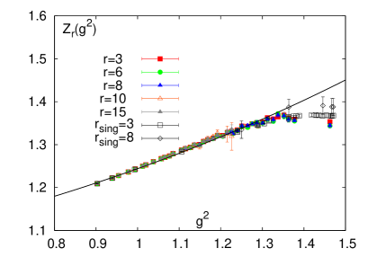
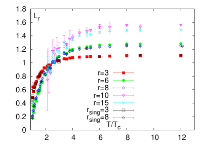
Figure 1: Left: renormalisation constants $Z_{r}(g^{2})$ for $r\leq 15$ obtained by the $N_{\tau}$-variation method and for $r=3,8$ from the matching of the $Q\bar{Q}$-singlet free energies to the $T=0$ potential. Right: renormalised Polyakov loop.

Realizing that the renormalization constants only depend on the bare coupling [3], $Z_{r}(g^{2})$, the renormalized Polyakov loop can be obtained from the bare loops at different $N_{\tau}$. As any renormalization procedure is fixed up to a multiplicative constant , i. e. $L_{r}^{c}=L_{r}e^{-c/2T}$, we fix the value of the renormalized Polyakov loop at the highest temperature ($12T_{c}$) to the value obtained by the renormalization procedure used in [1]. We obtain the corresponding $Z_{r}(g^{2})$ for the different $N_{\tau}$ and can use them to renormalize the Polyakov loop at a different $T$ by varying $N_{\tau}$. At this new value of $T$, all values of $L_{r}^{(b)}$ for different $N_{\tau}$ can be renormalized to this value and determine a new series of $Z_{r}(g^{2})$ at different couplings corresponding to this $T$ at the various $N_{\tau}$. The same method can now be performed for all representations. We only have to fix the value at the highest temperature, where we assume Casimir scaling,

$$L_{r}(12T_{c})\equiv(L_{3}(12T_{c}))^{d_{D}},$$ (4)

where $d_{D}=C_{2}(r)/C_{2}(3)$. In perturbation theory the renormalization constants are related by Casimir scaling (at least up to two loop order ($\alpha_{s}^{3}$) [4]). Therefore we define them through

$$L_{r}=(Z_{r}(g^{2}))^{N_{\tau}d_{D}}L_{r}^{(b)}.$$ (5)

The results for $Z_{r}(g^{2})$ and $L_{r}(T)$ are shown in fig. 1. We observe that the renormalization constants obtained independently in this way agree surprisingly well in the whole coupling range analyzed here. Furthermore they also agree with the renormalization constants obtained for $r=3$ and $r=8$ with the renormalization procedure outlined in [1], that defines the renormalized fundamental Polyakov loop by renormalizing the singlet free energy at small distances to the (perturbative) zero temperature potential. The solid line in fig. 1(left) shows the result of a best-fit analysis to the perturbative inspired ansatz

$$Z_{r}(g^{2})=\exp\left(g^{2}\frac{8}{3}Q^{(2)}+g^{4}Q^{(4)}\right),$$ (6)

where we find $Q^{(2)}=0.0576(25)$ and $Q^{(4)}=0.0639(68)$.

If Casimir scaling is realized, the renormalization constants for different representations should agree, i. e.

$$Z_{r}(g^{2})=Z_{3}(g^{2}).$$ (7)

As we have observed that the renormalization constants are related by Casimir scaling, we can now analyze if Casimir scaling also holds for the Polyakov loops. Through (5) it is equivalent to analyze this for the bare or renormalized loops. If Casimir scaling for the bare Polyakov loops is realized,

$$\left\langle L_{r}^{(b)}\right\rangle=\left\langle L_{3}^{(b)}\right\rangle^{d_{r}},$$ (8)

we expect the quantity $\langle L_{r}^{(b)}\rangle^{1/d_{r}}$ to be independent of the representation $r$. In fig. 2(left) we show the results of our calculations. We observe all data to collapse onto a single curve for temperatures down close to the critical temperature, confirming (8) to be valid within errors for representations $r=3,6,8,10,15$ above $T_{c}$.

3 The adjoint Polyakov loop in the confined phase

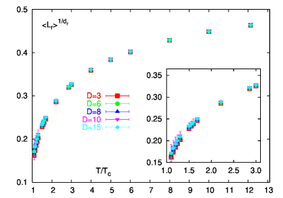
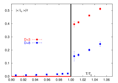
Figure 2: Left: bare Polyakov loops for $r\leq 15$ with cubic spline above $T_{c}$. Right: renormalized fundamental and adjoint Polyakov loop for temperatures around $T_{c}$.

While the Polyakov loop in the fundamental representation vanishes in the thermodynamic limit in the confined phase, for all triality-zero representations (r=8,10,27), one expects to see string breaking below $T_{c}$ also in pure gauge theory [2], and hence a non-vanishing Polyakov loop in the infinite volume limit.

We have analyzed the volume dependence of the adjoint Polyakov loops and found that for $N_{\sigma}=32$ the infinite volume limit is already reached. We can therefore use the $N_{\sigma}=32$ data to obtain the infinite volume, renormalized adjoint Polyakov loop below $T_{c}$. Fig. 2(right) shows $\left\langle L_{8}\right\rangle$ around $T_{c}$. While the adjoint Polyakov loop is small but non-zero for all temperatures analyzed here, the fundamental renormalized Polyakov loop is zero below $T_{c}$.

For the other triality-zero representations ($r=10,27$), we cannot give the infinite volume limit below $T_{c}$, since the corresponding $\left\langle L_{r}\right\rangle$ still show volume dependences on the analyzed lattices.

4 Conclusion and Outlook

We have investigated the Polyakov loop and free energies of static quark-antiquarks in different representations of SU(3) in pure gauge at finite $T$. Above the crititcal temperature the Polyakov loop in different representations shows Casimir scaling down close to $T_{c}$. Moreover, we were able to test the renormalization scheme proposed in [1] for the fundamental Polyakov loops and could generalize it to arbitrary representations. Furthermore we also demonstrate that the renormalization constants only depend on the bare coupling, at least up to $g^{2}\approx 1.3$. Below the critical temperature we were able to show, that the adjoint Polyakov loop is finite in the infinite volume limit and extract its infinite volume renormalized value. For higher triality-zero representations, no definite answer could be given within this work. We note that the renormalization procedure discussed here is based solely on gauge independent quantities and that the agreement of the renormalized Polyakov loops and the renormalization constants with the procedure outlined in [1] suggests that also in that procedure no gauge dependence exists. For discussion on potential gauge dependencies see [5, 6]. A different renormalization procedure was proposed in [7].

References

- [1] O. Kaczmarek et al., Phys. Lett. B543 (2002) 41.
- [2] G. S. Bali, Phys. Rev. D62 (2000) 114503.
- [3] R. A. Brandt et al., Phys. Rev. D 24, 879 (1981).
- [4] Y. Schroder, Phys. Lett. B447 (1999) 321.
- [5] O. Philipsen, Phys. Lett. B 535, 138 (2002)
- [6] O. Jahn and O. Philipsen, Phys. Rev. D 70, 074504 (2004)
- [7] A. Dumitru et al., Phys. Rev. D 70, 034511 (2004)