Accelerating Dynamical Fermion Computations using the
Rational Hybrid Monte Carlo (RHMC) Algorithm
with Multiple Pseudofermion Fields

Abstract

There has been much recent progress in the understanding and reduction of the computational cost of the Hybrid Monte Carlo algorithm for Lattice QCD as the quark mass parameter is reduced. In this letter we present a new solution to this problem, where we represent the fermionic determinant using $n$ pseudofermion fields, each with an $n^{\mbox{\tiny{th}}}$ root kernel. We implement this within the framework of the Rational Hybrid Monte Carlo (RHMC) algorithm. We compare this algorithm with other recent methods in this area and find it is competitive with them.

The motivation for this work is the need for faster algorithms to perform lattice QCD calculations near the chiral limit. To include the effects of fermions in our calculations we are required to invert the Dirac operator, which is a very large sparse matrix: as the fermion mass is decreased the computational cost increases with the condition number of the matrix $\kappa(\mathcal{M})$. Lattice QCD calculations involve the integration of Hamilton’s equations of motion, and the fermionic force acting on the gauge fields also increases with decreasing fermion mass. To maintain the stability of the integrator the integration step size must be reduced, thus increasing the cost. In this paper we shall not address the first of these problems, but shall introduce a method to bring the latter under control. This work is related to similar work by Hasenbusch Hasenbusch:2001ne , but our method requires less parameter tuning.

When performing a lattice QCD simulation, we desire gauge field configurations $U$ distributed according to the probability density

$$P(U)=\frac{1}{Z}e^{-S_{\mbox{\tiny g}}(U)}\mathop{\rm det}\mathcal{M}(U),$$

where $S_{\mbox{\tiny g}}$ is the pure gauge action and $\mathop{\rm det}\mathcal{M}$ is the determinant of the Dirac operator $\mathcal{M}=({\mathchoice{\mbox{D}\kern-6.49994pt\raise 0.6458pt\hbox{/}\kern 1.49994pt}{\mbox{D}\kern-6.49994pt\raise 0.6458pt\hbox{/}\kern 1.49994pt}{\mbox{\scriptsize D}\kern-5.0pt\raise 0.6458pt\hbox{\scriptsize/}}{\mbox{\tiny D}\kern-4.19998pt\raise 0.6458pt\hbox{\tiny/}}}+m)^{\dagger}({\mathchoice{\mbox{D}\kern-6.49994pt\raise 0.6458pt\hbox{/}\kern 1.49994pt}{\mbox{D}\kern-6.49994pt\raise 0.6458pt\hbox{/}\kern 1.49994pt}{\mbox{\scriptsize D}\kern-5.0pt\raise 0.6458pt\hbox{\scriptsize/}}{\mbox{\tiny D}\kern-4.19998pt\raise 0.6458pt\hbox{\tiny/}}}+m)$, which appears after integrating out the Grassmann-valued quark fields. The operator D/ is the discretized covariant derivative, and $m$ is the fermion mass. We represent the determinant as a pseudofermion Gaussian functional integral ($\mathop{\rm det}\mathcal{M}\propto\int d\phi\,d\phi^{\dagger}\,\exp{\left(-\phi^{\dagger}\mathcal{M}^{-1}\phi\right)}$), giving the probability density

$$P(U,\phi)=\frac{1}{Z^{\prime}}e^{-S_{\mbox{\tiny g}}(U)-S_{\mbox{\tiny f}}(\mathcal{M})}=\frac{1}{Z^{\prime}}e^{-\mathop{S_{\rm eff}}}.$$

Almost all techniques for generating gauge configurations consist of variants of Hybrid algorithms, these being algorithms which combine momentum and pseudofermion refreshment heatbaths with molecular dynamics (MD) integration of the gauge field. The latter is done through the introduction of a “fictitious” momentum field $\pi$, with which we define the Hamiltonian $H={\mathchoice{\textstyle{1\over 2}}{\scriptstyle{1\over 2}}{\scriptscriptstyle{1\over 2}}{1/2}}\pi^{2}+\mathop{S_{\rm eff}}$. The gauge fields can then be allowed to evolve for a time $\tau$ by integrating Hamilton’s equations. Hybrid algorithms are ergodic and their fixed point is close to but not precisely the desired one. This discrepancy is due to the inexact integration of Hamilton’s equations: the Hamiltonian is conserved to $O(\delta\tau^{k})$, where $k$ is determined by the order of the integration scheme used. Hybrid algorithms which use area preserving and reversible (symplectic and symmetric) integrators can be made exact through the addition of a Metropolis acceptance test at the end of the MD trajectory, which stochastically corrects for these errors. The Hybrid Monte Carlo algorithm (HMC) algorithm Duane:1987de is the de facto method for generating the required probability distribution, of which a single update consists of the following Markov steps

• Momentum refreshment heatbath using Gaussian noise ($P(\pi)\propto e^{-\pi^{2}/2}$).

• Pseudofermion refreshment ($P(\phi)\propto({\mathchoice{\mbox{D}\kern-6.49994pt\raise 0.6458pt\hbox{/}\kern 1.49994pt}{\mbox{D}\kern-6.49994pt\raise 0.6458pt\hbox{/}\kern 1.49994pt}{\mbox{\scriptsize D}\kern-5.0pt\raise 0.6458pt\hbox{\scriptsize/}}{\mbox{\tiny D}\kern-4.19998pt\raise 0.6458pt\hbox{\tiny/}}}+m)^{\dagger}\eta$, where $P(\eta)\propto e^{-\eta^{\dagger}\eta}$).

• MDMC, which consists of

  • MD trajectory consisting of $\tau/\delta\tau$ steps.

  • Metropolis accept/reject with probability $P_{\mbox{\tiny acc}}=\min(1,e^{-\delta H})$.

When updating the momentum there are contributions to the force from both the pure gauge part of the action $\partial S_{\mbox{\tiny g}}/\partial U$, and the fermionic part $\partial S_{\mbox{\tiny f}}/\partial U$. As the fermion mass is decreased the latter becomes the dominant contribution. To avoid an instability in the integrator and to maintain a non-negligible acceptance rate we must reduce the step size $\delta\tau$: this makes the computation very expensive since at every MD step we must solve a large system of linear equations.

Since the fermion determinant is represented using a single pseudofermion configuration selected from a Gaussian heatbath, the variance of this stochastic estimate will lead to statistical fluctuations in the fermionic force: the pseudofermionic force may be larger than the exact fermionic force, which is the derivative $\partial\mathop{\rm tr}\mathop{\rm ln}\mathcal{M}(U)/\partial U$ with respect to the gauge field $U$. This means that the pseudofermionic force may trigger the instability in the integrator even though the exact force would not.

An obvious way of ameliorating this effect is to use $n>\nobreak 1$ pseudofermion fields to sample the functional integral: this is achieved simply by writing

$$\mathop{\rm det}\mathcal{M} = [\mathop{\rm det}\mathcal{M}^{1/n}]^{n}$$

$$\propto \prod_{j=1}^{n}d\phi_{j}\,d\phi^{\dagger}_{j}\,\exp{\left(-\phi^{\dagger}_{j}\mathcal{M}^{-1/n}\phi_{j}\right)},$$

that is introducing $n$ pseudofermion fields $\phi_{j}$ each with kernel $\mathcal{M}^{-1/n}$.

It is well known that the instability in the integrator is triggered by isolated small modes of the fermion kernel Joo:2000dh . These modes are of magnitude $O(1/m^{2})$ with the standard kernel; with our multiple pseudofermion approach these modes are now $O(1/m^{2})^{1/n}$, and so are vastly reduced in magnitude. We would thus expect that the instability is shifted to occur at a far greater integrating step size.

If we make the simple-minded estimate that the magnitude of the fermion force is proportional to the condition number of the fermion matrix multiplied by the step size, then we can find the optimum value of $n$. We must keep the maximum force fixed so as to avoid the instability in the integrator, so we may increase the integration step size to $\delta\tau^{\prime}$ such that $n\kappa(\mathcal{M})^{1/n}\delta\tau^{\prime}=\kappa(\mathcal{M})\,\delta\tau$, where we have used the fact that $\kappa(\mathcal{M}^{1/n})=[\kappa(\mathcal{M})]^{1/n}$. At constant trajectory length and acceptance rate, and hence constant autocorrelation times, the cost of an HMC trajectory is proportional to the ratio $n/\delta\tau^{\prime}$, and thus is minimized by choosing $n$ so as to minimize $n\,\delta\tau/\delta\tau^{\prime}=n^{2}\kappa(\mathcal{M})^{\frac{1}{n}-1}$, which leads to the condition $n_{\mbox{\tiny opt}}={\mathchoice{\textstyle{1\over 2}}{\scriptstyle{1\over 2}}{\scriptscriptstyle{1\over 2}}{1/2}}\mathop{\rm ln}\kappa(\mathcal{M})$, corresponding to cost reduction by a factor of $n\,\delta\tau/\delta\tau^{\prime}=\left[e\mathop{\rm ln}\kappa(\mathcal{M})\right]^{2}/\left[4\kappa(\mathcal{M})\right]$.

Our method is to apply the Rational Hybrid Monte Carlo (RHMC) algorithm Clark:2003na to generate gauge field and pseudofermion configurations distributed according to the probability density

$$P(U,\phi_{1},\ldots,\phi_{n})=\frac{1}{Z}\exp{\left[-S_{\mbox{\tiny g}}(U)-S_{\mbox{\tiny f}}(\mathcal{M},n)\right]}$$

where $S_{\mbox{\tiny f}}(\mathcal{M},n)=\sum_{j=1}^{n}\phi^{\dagger}_{j}\mathcal{M}^{-1/n}\phi_{j}$. Optimal Chebyshev rational approximations are used to evaluate the matrix functions, and we proceed as we would for conventional HMC Duane:1987de . If written in partial fraction form $r(\mathcal{M})=\sum_{k=1}^{l}\alpha_{k}/(\mathcal{M}+\beta_{k})$, the rational function can be evaluated using a multi-shift solver Frommer:1995ik ; Jegerlehner:1996pm . The resulting computational cost per pseudofermion field very similar to HMC  since the shifts $\beta_{k}$ are all positive, the most costly shift being that which is closest to zero. Remarkably, all the coefficients $\alpha_{k}$ are also positive, so the procedure is numerically stable.

At this point it is worth comparing our method to the multiple pseudofermions through mass preconditioning method, or the so called Hasenbusch trick Hasenbusch:2001ne . In the latter, the fermion determinant is written $\mathop{\rm det}\mathcal{M}=\mathop{\rm det}\hat{\mathcal{M}}\mathop{\rm det}[\mathcal{M}/\hat{\mathcal{M}}]$, where the mass parameter used in $\hat{\mathcal{M}}$ is larger than that in $\mathcal{M}$. The original idea behind this method was to tune the mass of the dummy operator $\hat{\mathcal{M}}$ such that the operators had a similar condition number Hasenbusch:2002ai . An increase in step size would then be possible for the same reasons given above. The advantage with this method compared to RHMC is that the extra operators introduced are heavier, and hence cheaper to evaluate compared to the original kernel. Recently, larger speedups have been found through tuning the dummy mass(es) such that the action constituents with the greatest forces are those which are cheapest to evaluate, i.e., the heaviest Urbach:2005ji . A multi-level integration scheme Sexton:1992nu is then used which evaluates the cheaper and dominant forces more frequently than the more expensive and smaller forces. Tuning the mass parameters with both of these methods requires some effort, and even more so as further dummy operators are introduced. This compares to our RHMC method which requires no tuning of the extra operators since all operators are identical.

RHMC has the added virtue in that it allows the inclusion of less fermions than are described by the kernel $\mathcal{M}$ (typically this represents two fermions). For example to simulate full QCD, we are required to include the contribution from the light quark pair (at present we always assume $m_{u}=m_{d}$) and the strange quark. Traditionally the inclusion of the strange quark has proved problematic, and the use of an inexact algorithm Gottlieb:1987mq has been required. An alternative has been to use polynomial approximations, but such an approach requires either a very large degree polynomial ($>O(1000)$ for light quarks), or a correction step which is applied with the acceptance test or when making measurements deForcrand:1996ck ; Frezzotti:1997ym . RHMC allows the strange quark to be included simply through the use of the rational approximation $\sqrt{\mathcal{M}}\approx r(\mathcal{M})$, and because of the high accuracy of rational approximations, no correction step is required.

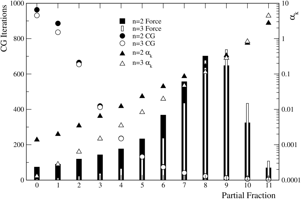
Figure 1: The variation of the force magnitude ($L_{2}$ norm), conjugate gradient (CG) cost and $\alpha_{k}$ parameter for each partial fraction with $n=2,3$ pseudofermions ($24^{3}\times 32$ lattice, $\beta=5.6$, $\kappa=0.15800$, CG residual $=10^{-6}$ for all shifts).

An important observation that has been made with prior use of RHMC is that the derivatives of the partial fractions have vastly different magnitudes Clark:2005sq . In Figure 1 we show the variation of magnitude of the force with each partial fraction, in order of increasing shift. The surprise is that the smallest shifts contribute least to the total fermion force. Also included on the plot is the number of conjugate iterations required in the multi-shift solver to reduce the residual for each shifted system by six orders of magnitude relative to the source. The most expensive constituents of the fermion force actually have the smallest magnitude. This effect may in part due to the fact that the density of states of the Dirac operator is greatest in the bulk, but principally because of the nature of the rational coefficients. This latter effect is enhanced as $n$ is increased because the coefficients $\alpha_{k}$ become smaller for light shifts, and larger for heavier shifts (see Figure 1).

We can make use of this observation by two methods. In the spirit of Urbach:2005ji we can construct a multi-timescale numerical integrator that assigns a larger step size to the small shifts, the ratio of the two step sizes being chosen such that the product $F\delta\tau$ is the same. In practice we have found the simpler approach where the smaller shifts are given a looser stopping condition than the heavier shifts while keeping the step size the same for all shifts, to be a more effective approach. It is important to mention that loosening the stopping condition of the poles has no effect on the reversibility of the molecular dynamics Joo:2000dh . Here we are loosening the stopping condition of the smaller shifts which are less important for evaluating the total fermion force.

To test our hypothesis that the use of multiple pseudofermions removes the integrator instability, we produced the data shown in Figure 2 using a relatively modest lattice volume. On a logarithmic scale we plot the value of $\langle\delta H^{2}\rangle^{1/2}$ versus the step size for $n=1,2$ and $3$ pseudofermions. We used a multi-timescale integrator to isolate the effect of the fermions from that of the gauge action. For $n=1$ when the step size reaches $\delta\tau=0.066$, $\delta H$ explodes by four orders of magnitude, this corresponds to the value for which the instability is triggered. For $n=2$ and $3$ not only is energy conservation better, but also the instability has been removed.

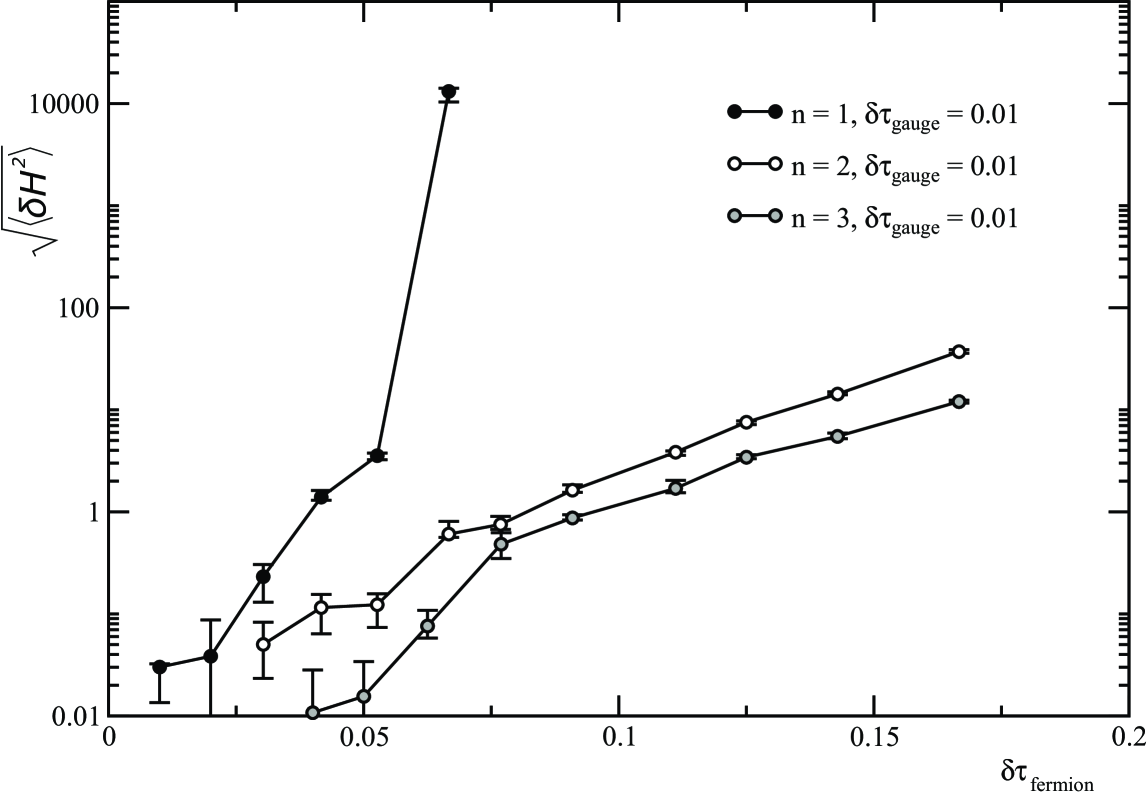
Figure 2: The variation of $\delta H$ with step size for $n=1,2,3$, the integrating step size has been fixed at approximately $\delta\tau=0.01$ (Wilson gauge action, Staggered fermions, $16^{4}$ lattice, $\beta=5.76$, $m=0.005$).

In conventional HMC the second order leapfrog integrator is usually found to be optimal, and the use of higher order integrators are found to decrease performance. Higher order integrators are more susceptible to the instability discussed before because they are constructed from longer sub-steps than the original leapfrog step. If multiple pseudofermions bring the instability under control, higher order integrators should now prove advantageous; this is indeed found to be the case. We have tried a variety of fourth order integrators: the fourth order Campostrini Campostrini:1989ac integrator and fourth order minimum norm integrators Takaishi:2005tz . While these all help we have generally found the fourth order minimum norm integrator (4MN5FV) to be optimal. Initial investigation has not found any gain from using a sixth order integrator, though this (or an even higher order integrator) should not be ruled out from future investigation.

$\kappa$	$n$	$l_{\mbox{\tiny{md}}}$	$l_{\mbox{\tiny{mc}}}$	Integrator	$\tau$	$\delta\tau$
0.15750	2	11	15	2MN	1.0	0.1
0.15800	3	12	16	4MN5FV	2.0	0.25
0.15825	3	12	16	4MN5FV	2.0	0.25

Table 1: Table of parameters used for this study. The 2MN integrator is the second order minimum norm integrator Takaishi:2005tz . For the MD the smallest two shifts had a CG residual of $10^{-4}$, $10^{-5}$ for the next two, and $10^{-6}$ for the remaining shifts. For all shifts the CG residuals were set to $10^{-10}$ for the heatbath and action evaluations.

				$\tau_{\mbox{\tiny{plaq}}}\cdot N_{\mbox{\tiny{mv}}}\times 10^{-4}$
			$N_{\mbox{\tiny{mv}}}\times$	This	Ref.	Ref.
$\kappa$	$\langle A\rangle$	$\tau_{\mbox{\tiny{plaq}}}$	$10^{-4}$	paper	Urbach:2005ji	Orth:2005kq
0.15750	0.755(9)	7(1)	1.37	9.59	9.00	19.075
0.15800	0.935(10)	4.9(8)	3.9	19.11	17.36	128.000
0.15825	0.911(12)	4.7(6)	11.2	52.50	56.50	—

Table 2: Table of results comparing RHMC with conventional HMC and the multiple timescale mass preconditioning presented in Urbach:2005ji . Our measure of cost is the product of the integrated autocorrelation of the plaquette $\tau_{\mbox{\tiny{plaq}}}$ with the number of Dirac operator applications per trajectory $N_{\mbox{\tiny{mv}}}$.

To test the efficiency of our final algorithm we choose the same parameters that have been used in recent publications Luscher:2005rx ; Urbach:2005ji : namely a $24^{3}\times 32$ lattice, using a Wilson gauge action ($\beta=5.6$) together with unimproved Wilson fermions with three different mass parameters.

A summary of our results compared to multi-timescale mass preconditioning Urbach:2005ji and conventional HMC Orth:2005kq can be seen in Table 2. Our algorithm is very similar in performance to that presented in Urbach:2005ji , and both of these algorithms are clearly superior to conventional HMC as expected. The results are also comparable with those of Lüscher Luscher:2005rx , but are far easier and more efficient to implement especially on fine grained parallel computers.

Conclusions

In this letter we have presented a simple improvement to the HMC algorithm to reduce the computation required for Lattice QCD calculations. This method leads to a large gain in performance relative to the conventional algorithm. At the physical parameters analyzed, our method is competitive with the mass preconditioning method presented in Urbach:2005ji ; moreover, the use of the RHMC algorithm permits the easy introduction of single quark flavors. In practice it is often advantageous to combine mass preconditioning with the present $n^{\mbox{\tiny{th}}}$ root method. The benefit that is gained from the improved HMC algorithms increases as the quark mass is reduced, and in this regime it would be interesting to further compare these algorithms. As the lattice volume is increased, we expect our method to prove more advantageous because of the improved volume dependence of higher order integrators (with a second order integrator, the cost of HMC is expected to scale $V^{5/4}$, whereas with a fourth order integrator the cost is expected to scale $V^{9/8}$ Creutz:1989wt ).

The importance of these results is that the cost to generate gauge field configurations with light fermions, which is the most costly part of lattice field theory computations, has been drastically reduced. This corresponds to more than a four fold decrease in computer time. These techniques also promise to lead to similar improvements in other fields where pseudofermion techniques are used for fermionic Monte Carlo computations.

References

- (1) Martin Hasenbusch. Phys. Lett., B519:177–182, 2001 (hep-lat/0107019).
- (2) S. Duane, A. D. Kennedy, B. J. Pendleton, and D. Roweth. Phys. Lett., B195:216–222, 1987.
- (3) Bálint Jóo et al. Phys. Rev., D62:114501, 2000 (hep-lat/0005023).
- (4) M. A. Clark and A. D. Kennedy. Nucl. Phys. Proc. Suppl., 129:850–852, 2004 (hep-lat/0309084).
- (5) Andreas Frommer, Bertold Nockel, Stephan Gusken, Thomas Lippert, and Klaus Schilling. Int. J. Mod. Phys., C6:627–638, 1995 (hep-lat/9504020).
- (6) Beat Jegerlehner. 1996 (hep-lat/9612014).
- (7) M. Hasenbusch and K. Jansen. Nucl. Phys., B659:299–320, 2003 (hep-lat/0211042).
- (8) C. Urbach, K. Jansen, A. Shindler, and U. Wenger. Comput. Phys. Commun., 174:87–98, 2006 (hep-lat/0506011).
- (9) J. C. Sexton and D. H. Weingarten. Nucl. Phys., B380:665–678, 1992.
- (10) Steven A. Gottlieb, W. Liu, D. Toussaint, R. L. Renken, and R. L. Sugar. Phys. Rev., D35:2531–2542, 1987.
- (11) Philippe de Forcrand and Tetsuya Takaishi. Nucl. Phys. Proc. Suppl., 53:968–970, 1997 (hep-lat/9608093).
- (12) Roberto Frezzotti and Karl Jansen. Phys. Lett., B402:328–334, 1997 (hep-lat/9702016).
- (13) M. A. Clark, Ph. de Forcrand, and A. D. Kennedy. PoS, LAT2005:115, 2005 (hep-lat/0510004).
- (14) Massimo Campostrini and Paolo Rossi. Nucl. Phys., B329:753, 1990.
- (15) Tetsuya Takaishi and Philippe de Forcrand. Phys. Rev., E73:036706, 2006 (hep-lat/0505020).
- (16) Boris Orth, Thomas Lippert, and Klaus Schilling. Phys. Rev., D72:014503, 2005 (hep-lat/0503016).
- (17) Martin Lüscher. Comput. Phys. Commun., 165:199–220, 2005 (hep-lat/0409106).
- (18) Michael Creutz and Andreas Gocksch. Phys. Rev. Lett., 63:9, 1989. BNL-42601.