CERN-PH-TH/2006-134

Using 4 flavors of staggered fermions at infinite gauge coupling, we compare various analytic results for the hadron spectrum with exact Monte Carlo simulations. Agreement with Ref. [4] is very good, at the level of a few percent.

Our results give credence to a discrepancy between the baryon mass and the critical chemical potential, for which baryons fill the lattice at zero temperature and infinite gauge coupling. Independent determinations of the latter set it at about 30% less than the baryon mass. One possible explanation is that the nuclear attraction becomes strong at infinite gauge coupling.

1 Introduction

The strong coupling limit of lattice QCD can provide valuable insight, as Wilson showed by proving the area-law behaviour for the Wilson loop in that regime [1]. Analytic integration over the gauge link variables becomes feasible in this limit. Within some reasonable approximation (typically mean field), one can then calculate analytically the hadron spectrum. The result turns out to be not too different from the continuum QCD spectrum. This has been the subject of numerous works [2, 3, 4, 5]. To the best of our knowledge however, these analytic results involving different approximation schemes have never been compared with the results of numerical simulations in the infinite coupling limit ($\beta\equiv 6/g^{2}=0$). Here, we perform such a comparison for the case of 4 flavors of staggered fermions with SU(3) gauge group.

In addition, we are motivated by a puzzle in the phase diagram of QCD as a function of temperature $T$ and chemical potential $\mu$. This phase diagram also can be determined analytically when $\beta=0$, and has been investigated by use of increasingly sophisticated approximations over the years [6]-[11]. At zero temperature, a first-order transition is predicted to take place, where the baryon density jumps from zero to saturation (1 baryon per lattice site). The corresponding critical quark chemical potential for massless quarks has been calculated in the mean-field approximation, which yields $\mu_{c}a\sim 0.66$ [6]. This analytic prediction has also been confirmed by numerical simulation of a gas of loops, the monomer-dimer-polymer ensemble, whose partition function is identical to that of lattice QCD with staggered fermions at $\beta=0$ [12], and by the Glasgow reweighting method [13]. The numerical simulation of [12] gives $\mu_{c}a=0.63(2)$ in the chiral limit and $0.690(15)$ at $m_{q}a=0.1$. The result from [13] is $\mu_{c}a=0.687(15)$ at $m_{q}a=0.1$. At first sight, this excellent agreement between mean-field and Monte Carlo is very satisfying. On second thought, however, it is rather mysterious. One would expect the transition to occur when ($3\mu$) exceeds the free energy required to create an additional baryon, which is equal to its mass at $T=0$. Now, every analytic prediction for the nucleon mass $m_{N}$ gives a value $(m_{N}a)$ very close to 3 so that $(\mu_{c}a)$ should be very close to 1. The values reported above are considerably smaller. Among the various explanations for this puzzle, we want to check the validity of the analytic approximations: is the nucleon mass really close to 3 in the strong coupling limit, or is it close to $3\mu_{c}a$ instead?

In the next section (Sec.II), we review the analytic approximations which have been proposed for the hadron spectrum. Then (Sec.III) we present our simulation results and compare our numerical results to the analytic predictions in Table I. Conclusions follow.

2 Overview of analytic approaches

In the strong coupling limit, the gauge field part of the action can be dropped because its coefficient is $\beta=0$, and the gauge link variables become random $SU(N)$ group elements. Then, gauge links give non-vanishing contributions only when a given link forms a part of an $SU(N)$ singlet combination. Using this property, one can construct either an effective action and derive the hadron spectrum from it [2, 3], or one can count the graphically relevant diagrams and obtain from them the hadron spectrum [4].

In [2, 3], the authors derive the effective action for $SU(3)$ in terms of meson and baryon degrees of freedom by integrating the gauge link variables out. Then, via systematic large-$d$ (the spacetime dimension) expansion of this effective action, the chiral condensate and the correlation functions of the composite mesonic and baryonic fields are obtained. The positions of poles in the zero momentum projected correlators give meson ($M_{M}$) and baryon ($M_{B}$) masses which can be summarized as follows:

$$\frac{1}{N}\langle\overline{\psi}\psi\rangle \approx \sqrt{\frac{2}{d}}(\overline{\lambda}-2\overline{m})$$ (1)

$$\cosh M_{M}a = d(\overline{\lambda}^{2}-1)+2k+1,$$ (2)

$$\sinh M_{B}a = \frac{1}{2}\overline{\lambda}^{N}(2d)^{\frac{N}{2}}$$ (3)

where $\overline{\lambda}=\overline{m}+\sqrt{\overline{m}^{2}+1}$, $\overline{m}=ma/\sqrt{2d}$, $ma$ is the dimensionless quark mass, and $k=0,1,2,3$ gives access to four meson channels, to which are assigned the physical meaning of the $\pi$, $\rho$, $a_{1}$, $a_{0}/f_{0}$ respectively. For small $ma\ll\sqrt{2d}$,

$$\langle\overline{\psi}\psi\rangle \approx 2.12-0.75ma$$ (4)

$$(M_{\pi}a)^{2} \approx 5.66ma$$ (5)

$$M_{\rho}a \approx 1.76+ma$$ (6)

$$M_{a_{1}}a \approx 2.29+0.58ma$$ (7)

$$M_{a_{0}/f_{0}}a \approx 2.63+0.41ma$$ (8)

$$M_{B}a \approx 3.12+1.06ma$$ (9)

Leading $1/d$ corrections were obtained in [5], yielding for $d=4$, $N=3$:

$$\langle\overline{\psi}\psi\rangle \approx 1.99-0.56ma$$ (10)

$$(M_{\pi}a)^{2} \approx 4.60ma$$ (11)

$$M_{B}a \approx 2.93+1.99ma$$ (12)

and the masses of the other 3 mesons are unchanged. Leading corrections in $1/g^{2}$ were also obtained in Ref. [5]. They always come in the combination $1/(g^{2}N)$.

Perhaps this motivated the authors of [4] to try a different approach. They developed a graphical method for summing relevant, tree-like diagrams in the large-$N$ limit ($g^{2}N\rightarrow\infty$) at fixed $d$. They showed

$$\frac{1}{N}\langle\overline{\psi}\psi\rangle = \frac{dm_{r}-(2d-1)ma}{d^{2}+(ma)^{2}}$$ (13)

$$\cosh M_{M}a = \frac{((2d-1)-(2d-2){m_{r}}^{2}+{m_{r}}^{4})}{2{m_{r}}^{2}}+2k,$$ (14)

$$\sinh M_{B}a = \frac{1}{2}{m_{r}}^{N}$$ (15)

where $m_{r}=ma+\sqrt{(ma)^{2}+2d-1}$ and $k=0,1,2,3$. Again, for small $ma\ll\sqrt{2d-1}$, one obtains

$$(M_{\pi}a)^{2} \approx 4.54ma$$ (16)

$$M_{\rho}a \approx 1.76+0.81ma$$ (17)

$$M_{a_{1}}a \approx 2.63+0.32ma$$ (18)

$$M_{a_{0}/f_{0}}a \approx 2.29+0.46ma$$ (19)

$$M_{B}a \approx 2.91+1.14ma$$ (20)

The three sets of predictions are collected in Table I below, where they are denoted respectively “M.F.”(mean field)  [2, 3], “$1/d$-corr.” [5] and “$d=4$, large-$N$” [4]. The last two columns show our Monte Carlo results, presented in the next section, for the quenched and the full QCD theories.

Table 1: Comparison of hadron properties.

	$m_{q}a$	M.F.	$1/d$-corr.	$d=4$	MC results	MC results
		[2, 3]	[5]	large-$N$ [4]	quenched	$N_{f}=4$
average	0.1	–	–	–	0.00001(4)	0.00603(2)
plaquette	0.05	–	–	–	same	0.00656(3)
	0.025	–	–	–	same	0.00682(3)
	0.1	2.0463	1.9325	1.9281	1.9295(5)	1.9172(2)
$\langle\overline{\psi}\psi\rangle$	0.05	2.0838	1.9606	1.9562	1.9574(7)	1.9413(3)
	0.025	2.1026	1.9747	1.9703	1.9710(11)	1.9520(6)
	0.1	0.7521	0.6780	0.6735	0.6776(1)	0.6780(1)
$m_{\pi}$	0.05	0.5318	0.4794	0.4762	0.4778(1)	0.4784(1)
	0.025	0.3761	0.3390	0.3367	0.3374(1)	0.3379(1)
	0.1	1.863	1.863	1.841	1.847(2)	1.831(2)
$m_{\rho}$	0.05	1.813	1.813	1.801	1.802(4)	1.774(4)
	0.025	1.788	1.788	1.780	1.768(6)	1.779(7)
	0.1	2.350	2.350	2.336	2.337(6)	2.276(6)
$m_{a_{1}}$	0.05	2.321	2.321	2.313	2.317(9)	2.274(10)
	0.025	2.307	2.307	2.302	2.325(18)	2.300(19)
	0.1	2.675	2.675	2.662	2.637(16)	2.511(23)
$m_{a_{0}/f_{0}}$	0.05	2.654	2.654	2.646	2.588(27)	2.551(27)
	0.025	2.644	2.644	2.638	2.598(51)	2.636(47)
	0.1	3.225	3.129	3.024	2.961(3)	2.931(3)
$m_{N}$	0.05	3.172	3.030	2.967	2.890(4)	2.863(5)
	0.025	3.146	2.980	2.939	2.883(8)	2.831(10)

3 Numerical results

We have simulated the partition function $Z=\int{\cal D}U~{}e^{-S}$, with the staggered action $S$:

$$S=\sum_{x}[\frac{1}{2}\sum_{\mu}\eta_{\mu}(x)\{\overline{\psi}(x)U_{\mu}(x)\psi(x+\hat{\mu})-\overline{\psi}(x+\hat{\mu}){U_{\mu}}^{\dagger}(x)\psi(x)\}+ma\overline{\psi}\psi(x)]$$ (21)

with $\eta_{\mu}(x)=(-)^{x_{1}+..+x_{\mu-1}}$, for 3 values of the quark mass ($ma=0.1,0.05$ and $0.025$), on an $8^{3}\times 16$ lattice. In each case, 500 decorrelated configurations on which we measured the quark condensate and the hadron correlators have been accumulated. Since, with staggered fermions, a given hadron correlator also contains contributions from its parity partner, we perform joint fits of the two correlators of parity partners [14]:

$$C_{1}(t) = A(e^{-m_{1}t}+e^{-m_{1}(T-t)})+(-1)^{t}B(e^{-m_{2}t}+e^{-m_{2}(T-t)})$$

$$C_{2}(t) = A^{\prime}(e^{-m_{2}t}+e^{-m_{2}(T-t)})+(-1)^{t}B^{\prime}(e^{-m_{1}t}+e^{-m_{1}(T-t)}).$$ (22)

For example, the $\pi$ channel correlator is fitted simultaneously with the scalar channel correlator, and the $\rho$ channel correlator with the pseudovector channel correlator by use of the 6-parameter fitting form of Eq.(22).

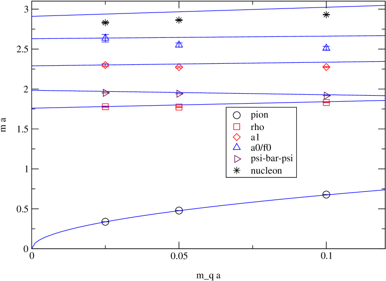
Figure 1: Hadron masses as a function of the quark mass $m_{q}a$. The solid lines show the predictions of Ref. [4].

A few words on our simulation algorithm may be useful. The 4-flavor theory can be simulated with standard Hybrid Monte Carlo. Nevertheless, we used RHMC [15], with two sets of pseudo-fermion fields each yielding $\sqrt{\det(M)}$ after integration. This decomposition allowed us to use a larger stepsize [16]. More importantly, the stopping criterion of our solver was set to the very loose value $1.0\times 10^{-2}$, while maintaining an acceptance $\sim 65$%. This great advantage of RHMC, recognized in [16], provides an important gain in efficiency.

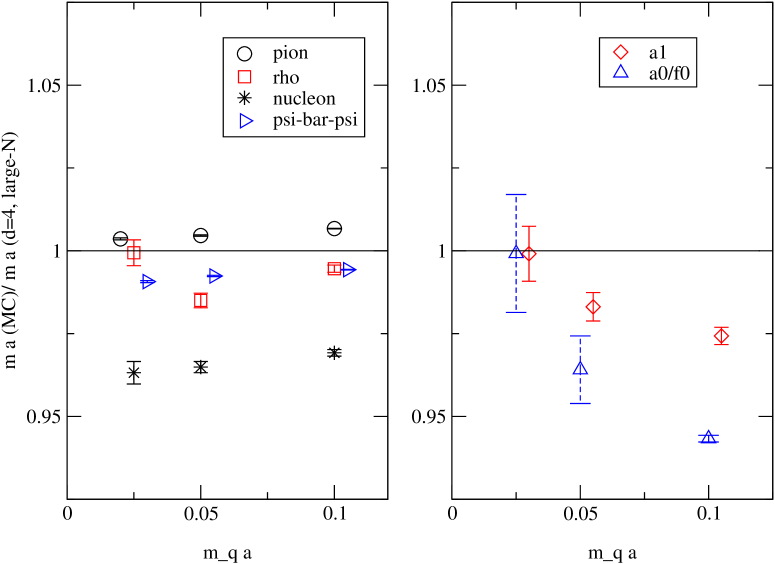
Figure 2: The ratio of our Monte Carlo data over the analytic result of Ref. [4], as a function of the quark mass $m_{q}a$. Some channels are horizontally shifted to avoid overlapping data points.

Our spatial volume is reasonably large compared to the pion mass ($m_{\pi}L=2.6$–$5.3$), and is very large compared to the nucleon mass ($L\sim 5.5$ fm). Thus we expect negligible finite-size effects on all observables except perhaps the pion mass, and analytic predictions obtained on an infinite lattice  [2, 3, 4, 5] can be directly compared with our numerical results. Our $m_{\pi}/m_{\rho}$ mass ratio ranges from 0.3703(5) down to 0.1899(7), compared to the physical value 0.179. So we are studying the light-quark regime. Note, however, that $m_{N}/m_{\rho}$ is about 1.6, close to the non-relativistic value $3/2$, and hardly changes with the quark mass. So the spectrum of strong coupling QCD is only crudely similar to that of continuum QCD.

Our results are collected in the rightmost two columns of Table I, for the quenched ($N_{f}=0$) and the full ($N_{f}=4$) theory. Ref. [4] counts all quark “tree graphs” which enclose zero area and is very similar to the quenched approximation. This motivated us to include quenched simulation results for comparison. Indeed, the tree graph resummation provides an excellent approximation to the quenched results. Differences (of about 2%) are visible in the nucleon mass only. In turn, the quenched and full QCD results are very close to each other, with the most difference (at the 5% level) in the $a_{0}/f_{0}$ channel.

The agreement between the full QCD results and the mean-field calculations [2, 3] is reasonable, and improves with $1/d$ corrections [5]. It is best in general with the large-$N$ approach of [4].

Figure 3: $m_{\rm baryon}a/3$ as a function of the quark mass $m_{q}a$ together with $\mu_{c}a$ (our data is added to the Figure from Ref. [13])

To illustrate the level of agreement with the predictions of [4], we show in Fig. 1 the masses we measured together with the analytic dependence of [4] as a function of the quark mass. In Fig. 2, we show the ratio of our measured values over those predicted by [4]. The agreement is better than within 1% for the chiral condensate $\langle\overline{\psi}\psi\rangle$ and the pion mass. The ratio for the rho mass varies non-monotonically, which is possibly caused by the crossing of the threshold for $\rho\to\pi\pi$ decay. For the nucleon, the Monte Carlo data is within 5% of [4]. Our determination of the scalar mass ($a_{0}/f_{0}$) is too poor to provide a real check. Interestingly, the lattice result agrees with the analytic result $m_{\pi}<m_{\rho}<m_{a_{1}}<m_{a_{0}/f_{0}}$, in contrast to the experimental ordering, $m_{\pi}<m_{\rho}<m_{a_{0}/f_{0}}<m_{a_{1}}$.

In Figure 3, we compare our nucleon mass with old Monte Carlo data for the critical, zero temperature quark chemical potential in infinite coupling QCD [12, 13]. The error bar for $1/3$ of our nucleon mass is smaller than the plot symbol. There is a clear, large difference between the critical quark chemical potential and $1/3$ of the nucleon mass.

4 Conclusions

On the whole, our study justifies the mean-field approximation used in [2, 3]. It also provides a beautiful confirmation of the approach of [4], which goes beyond mean-field and becomes exact when $g{{}^{2}}N\to\infty$. It may seem strange in fact that this $g{{}^{2}}N\to\infty$ approximation is so good (at the percent level), since virtual quark loops are absent in this approximation in contrast to the numerical simulation. The explanation, we believe, lies in the small plaquette average value. The dynamical quarks shift the plaquette away from the value zero which it would take in the quenched case, but only slightly. This shift increases very mildly for lighter quarks. The lightest quarks which we considered, $m_{q}a=0.025$, give a pion to rho mass ratio near the physical one, but yield a plaquette value of $0.00682(3)$ only. This is much less than the naive estimate based on a $1/(m_{q}a)$ expansion [21], which would predict an effective shift $\Delta\beta\approx 0.8$ in the gauge action, leading to a plaquette value ${\cal O}(0.1)$, about 15 times larger than measured. Thus, the price to pay for creating virtual quark loops remains high, and their effect on the spectrum is small. For the same reason, the quenched approximation turns out to be closer to full QCD at strong coupling than at weak coupling: at strong coupling, the ordering effect of the fermion loops is “drowned” in the disorder of the gluons.

As shown in Table I, the nucleon mass is just a bit smaller than 3. In particular, for $m_{q}a=0.1$ which is the quark mass used in the finite density simulations of [12, 13], the nucleon mass is 2.931(3) and one would expect the $T=0$ transition induced by a quark chemical potential to occur at $\mu_{c}=2.931(3)/3=0.977(1)$. However, the measured value for $\mu_{c}$ [12] is $0.690(15)$ ($0.687(15)$ in [13]). The discrepancy with the expected value is about 30%. In other words, the nucleon seems to have a free energy about 300 MeV less than its mass. Could this be caused by a strong attraction among nucleons [17, 18]? The weakness of the real-world nuclear interaction results from near-cancellation between the attractive omega exchange and the repulsive sigma exchange [19]. This cancellation may not occur when the parameters of QCD are modified. Of course, other, less extraordinary causes may be at work: non-zero temperature corrections, or even algorithmic problems as suggested in [20]. This line of investigation should be pursued further.

5 Acknowledgement

We thank Olivier Martin for correspondence. S.K. is supported in part by Korea Science and Engineering Foundation.

References

- [1] K. G. Wilson, Phys. Rev. D 10 (1974) 2445.
- [2] H. Kluberg-Stern, A. Morel and B. Petersson, Phys. Lett. B 114 (1982) 152; H. Kluberg-Stern, A. Morel and B. Petersson, Nucl. Phys. B 215 (1983) 527; H. Kluberg-Stern, A. Morel, O. Napoly and B. Petersson, Nucl. Phys. B 220 (1983) 447.
- [3] N. Kawamoto and J. Smit, Nucl. Phys. B 192 (1981) 100; J. Hoek, N. Kawamoto and J. Smit, Nucl. Phys. B 199 (1982) 495.
- [4] O. Martin, “Large N Gauge Theory At Strong Coupling With Chiral Fermion,” Ph.D. Thesis CALT-68-1048 (1983); O. Martin and B. Siu, Phys. Lett. B 131 (1983) 419; O. Martin, Phys. Lett. B 130 (1983) 411.
- [5] T. Jolicoeur, H. Kluberg-Stern, M. Lev, A. Morel and B. Petersson, Nucl. Phys. B 235 (1984) 455.
- [6] P. H. Damgaard, N. Kawamoto, and K. Shigemoto, Phys. Rev. Lett. 53, 2211 (1984). P. H. Damgaard, N. Kawamoto, K. Shigemoto, Nucl. Phys. B 264, 1(1986). P. H. Damgaard, D. Hochberg, and N. Kawamoto, Phys. Lett. B 158, 239 (1985).
- [7] E.-M. Ilgenfritz and J. Kripfganz, Z. Phys. C 29, 79(1985). G. Fäldt and B. Petersson, Nucl. Phys. B 265, 197(1986). N. Bilić, K. Demeterfi, and B. Petersson, Nucl. Phys. B 377, 651(1992). N. Bilić, F. Karsch, and K. Redlich, Phys. Rev. D 45, 3228(1992).
- [8] R. Aloisio, V. Azcoiti, G. Di Carlo, A. Galante, and A. F. Grillo, Nucl. PhysḂ 564, 489 (2000) [arXiv:hep-lat/9910015]. E. B. Gregory, S. H. Guo, H. Kröger, and X. Q. Luo, Phys. Rev. D 62, 054508 (2000) [arXiv:hep-lat/9912054].
- [9] Y. Umino, Phys. Rev. D 66, 074501 (2002) [arXiv:hep-ph/0101144]. B. Bringoltz and B. Svetitsky, Phys. Rev. D 68, 034501 (2003) [arXiv:hep-lat/0211018]. V. Azcoiti, G. Di Carlo, A. Galante, and V. Laliena, JHEP 0309, 014 (2003) [arXiv:hep-lat/0307019]. S. Chandrasekharan and F. J. Jiang, Phys. Rev. D 68, 091501 (2003) [arXiv:hep-lat/0309025].
- [10] Y. Nishida, Phys. Rev. D 69 (2004) 094501 [arXiv:hep-ph/0312371].
- [11] N. Kawamoto, K. Miura, A. Ohnishi and T. Ohnuma, [arXiv:hep-lat/0512023].
- [12] F. Karsch and K. H. Mutter, Nucl. Phys. B 313 (1989) 541.
- [13] I. M. Barbour, S. E. Morrison, E. G. Klepfish, J. B. Kogut and M. P. Lombardo, Phys. Rev. D 56, 7063 (1997) [arXiv:hep-lat/9705038].
- [14] S. Kim and D. K. Sinclair, Phys. Rev. D 48 (1993) 4408.
- [15] M. A. Clark and A. D. Kennedy, Nucl. Phys. Proc. Suppl. 129 (2004) 850 [arXiv:hep-lat/0309084].
- [16] M. A. Clark, P. de Forcrand and A. D. Kennedy, PoS LAT2005 (2005) 115 [arXiv:hep-lat/0510004].
- [17] I. M. Barbour, S. E. Morrison, E. G. Klepfish, J. B. Kogut and M. P. Lombardo, Nucl. Phys. Proc. Suppl. 60A (1998) 220 [arXiv:hep-lat/9705042].
- [18] N. Bilic, F. Karsch and K. Redlich, Phys. Rev. D 45 (1992) 3228.
- [19] G.E. Brown and A.D. Jackson, The Nucleon-Nucleon Interaction, North Holland (1977).
- [20] R. Aloisio, V. Azcoiti, G. Di Carlo, A. Galante and A. F. Grillo, Nucl. Phys. B 564 (2000) 489 [arXiv:hep-lat/9910015].
- [21] A. Hasenfratz and T. A. DeGrand, Phys. Rev. D 49 (1994) 466 [arXiv:hep-lat/9304001].