Calculating the hadronic vacuum polarization and leading hadronic contribution to the muon anomalous magnetic moment with improved staggered quarks

Abstract

We present a lattice calculation of the hadronic vacuum polarization and the lowest-order hadronic contribution (HLO) to the muon anomalous magnetic moment, $a_{\mu}=(g-2)/2$, using $2\!+\!1$ flavors of improved staggered fermions. A precise fit to the low-$q^{2}$ region of the vacuum polarization is necessary to accurately extract the muon $g\!-\!2$. To obtain this fit, we use staggered chiral perturbation theory, including a model to incorporate the vector particles as resonances, and compare these to polynomial fits to the lattice data. We discuss the fit results and associated systematic uncertainties, paying particular attention to the relative contributions of the pions and vector mesons. Using a single lattice spacing ensemble generated by the MILC Collaboration ($a=0.086$ fm), light quark masses as small as roughly one-tenth the strange quark mass, and volumes as large as (3.4 fm)³, we find $a_{\mu}^{\rm HLO}=(713\pm 15)\times 10^{-10}$ and $(748\pm 21)\times 10^{-10}$ where the error is statistical only and the two values correspond to linear and quadratic extrapolations in the light quark mass, respectively. Considering various systematic uncertainties not eliminated in this study (including a model of vector resonances used to fit the lattice data and the omission of disconnected quark contractions in the vector-vector correlation function), we view this as agreement with the current best calculations using the experimental cross section for $e^{+}e^{-}$ annihilation to hadrons, 692.4 (5.9) (2.4)$\times 10^{-10}$, and including the experimental decay rate of the tau lepton to hadrons, 711.0 (5.0) (0.8)(2.8)$\times 10^{-10}$. We discuss several ways to improve the current lattice calculation.

I Introduction

The current Standard Model of particle physics has had tremendous success in describing fundamental properties of Nature. Currently, precise determinations of physical quantities need to be performed in order to find discrepancies, if any, between theoretical predictions and experimental measurements. Many, but not all, quantities agree quite well between theory and experiment. In those cases where there are discrepancies, there is a need to reduce the errors on theoretical and experimental determinations of said quantities to see if these discrepancies are significant.

An excellent candidate for this improvement is the anomalous magnetic moment of the muon, $a_{\mu}=(g\!-\!2)/2$. The experimental world average is $a_{\mu}^{\rm exp}=116\,592\,080(5.4)(3.3)\!\times\!10^{-11}$ Bennett:2006fi ; bnl_g2 . The incredible precision of this measurement arises from the recent experiments at Brookhaven National Laboratory Bennett:2006fi . This number deviates from current theoretical predictions by 0.7 to 2.7 standard deviations, depending on the method of obtaining the Standard Model number (see the recent reviews g2REVIEW ; Davier:2004gb ).

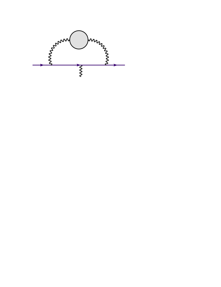
Figure 1: The lowest order diagram giving rise to QCD corrections to the muon $g\!-\!2$, at $\mathcal{O}(\alpha^{2})$. The blob represents all possible hadronic states.

The largest contribution to the error of the theoretical calculation lies in terms arising from QCD. The electroweak sector can be reliably calculated using perturbation theory but this is not the case for QCD. The first QCD contribution comes in at order ${\cal O}(\alpha^{2})$ ($\alpha=e^{2}/4\pi$ is the fine structure constant) shown in Figure 1 which is the hadronic contribution to the photon vacuum polarization. The next QCD contributions come in at ${\cal O}(\alpha^{3})$, the light-by-light contribution, which is currently being studied using lattice techniques LIGHTBYLIGHT , model calculations (e.g., Knecht:2001qg ; Hayakawa:2001bb ; Bijnens:2001cq ; Melnikov:2003xd ), and chiral perturbation theory Ramsey-Musolf:2002cy (for a recent review, see Ref. LightByLightReview ). We focus here on the larger of these two contributions, that coming from the QCD corrections to the photon vacuum polarization.

Since perturbation theory is unreliable for such hadronic contributions, for a long time one has relied on a dispersion relation to relate the imaginary part of the photon vacuum polarization to the real part Bouchiat:1961 ; Gourdin:1969dm which is needed in the diagram shown in Figure 1, using the experimental $e^{+}e^{-}\to{\rm hadrons}$ total cross-section to obtain the imaginary part. Additionally, one can relate the decay $\tau\to$ hadrons to the $e^{+}e^{-}$ cross section in the isospin limit g2REVIEW ; Davier:2004gb for a part of the energy range. Whether or not one includes the $\tau$ data gives the range of deviations discussed above between theory and experiment.

A purely theoretical calculation of $a_{\mu}^{\rm HLO}$ is desirable for at least three reasons: first, it is very important to corroborate the dispersive/experimental analysis with an alternative calculation in order to have confidence in the Standard Model comparison with experiment, and second, these calculations may eventually compete with or surpass the precision and accuracy of the dispersion relation/experiment combination. Finally, from a theoretical perspective it is quite interesting. Such theoretical calculations may in the future provide even more stringent tests between the Standard Model and experiment, a desirable outcome in the LHC era.

At present the only way to compute $a_{\mu}^{\rm HLO}$ theoretically in a model-independent way is to apply lattice gauge theory techniques to calculate the hadronic vacuum polarization. This has already been done in the quenched approximation with domain wall fermions g-2_1 and improved Wilson fermions QCDSF , as well as with dynamical ($2\!+\!1$ light flavors) “asqtad” staggered fermions g-2_2 ; g-2_3 . The main difficulty is that the largest uncertainties occur in the low-momentum region which gives the dominant contribution to $a_{\mu}^{\rm HLO}$. The goal of the current work is to incorporate staggered chiral perturbation theory (S$\chi$PT) SCHPT coupled to photons to derive a physically based fitting function to accurately describe this low-momentum region. Initial results from this fitting technique were presented in Lat05g-2 , and to our knowledge are the first chiral perturbation theory results for the vacuum polarization presented in the literature.

At this stage we must point out that an expansive and lively debate has recently taken place in the literature, and the lattice QCD community in general, concerning the theoretical validity of the staggered fermion formulation when applied to numbers of quarks different from a multiple of four, as in the present case of 2+1 flavors. We refer the interested reader to the most recent papers Shamir:2006nj ; Bernard:2006ee ; Bernard:2006vv ; Bernard:2006zw ; Hasenfratz:2006nw ; Creutz:2006ys , and also to the review by Sharpe at Lattice 2006 SHARPE_LATTICE . The important point stressed in the review is that staggered fermions are non-local for non-zero lattice spacing, but that the non-locality is a lattice artifact that vanishes in the continuum limit, provided the quark mass is not taken to zero first. Since we work at fixed lattice spacing, this may be cause for concern. As we shall see, the results presented below do not indicate signs of non-locality, and our future plans include taking the continuum limit when ensembles with smaller lattice spacing become available. We also plan to repeat our calculation with 2+1 flavors of domain wall fermions as a final check.

This paper is outlined as follows. We discuss in Sec. II the basic details of the lattice calculation of the vacuum polarization and how to use this to extract the lowest order hadronic contribution to the muon $g\!-\!2$. In Sec. III we discuss staggered chiral perturbation theory coupled to photons as external fields, and compute the one-loop pion and kaon contribution to the photon vacuum polarization. We find here that this is not an adequate description of the lattice data, and in Sec. IV we incorporate into the chiral perturbation theory the lightest vector fields, whose contribution to the vacuum polarization we find dominates over the pions. Sections V and  VI include our discussion of the fits, final results for the muon $g\!-\!2$ for this lattice spacing, and systematic uncertainties in the calculation. We conclude our study in Sec. VII.

II Lattice Calculation of the muon $g\!-\!2$

In the continuum, Euclidean and gauge invariance along with the Ward-Takahashi identity allow us to write the vacuum polarization tensor in momentum space as

$$\Pi_{\mu\nu}(q)=(q^{2}\delta_{\mu\nu}-q_{\mu}q_{\nu})\Pi(q^{2})\ .$$ (1)

We can use $\Pi(q^{2})$ as defined above in the space-like region to calculate the lowest order contribution to the muon $g\!-\!2$ from the expressions g-2_1

$$a_{\mu}^{\rm HLO} = \left(\frac{\alpha}{\pi}\right)^{2}\int_{0}^{\infty}dK^{2}f(K^{2})\hat{\Pi}(K^{2})\ ,$$ (2)

$$f(K^{2}) = \frac{m^{2}_{\mu}K^{2}Z^{3}\left(1-K^{2}Z\right)}{1+m^{2}_{\mu}K^{2}Z^{2}}\ ,$$ (3)

$$Z = -\frac{K^{2}-\sqrt{K^{4}+4m^{2}_{\mu}K^{2}}}{2m^{2}_{\mu}K^{2}}\ ,$$ (4)

$$\hat{\Pi}(K^{2}) = 4\pi^{2}\sum_{i}Q^{2}_{i}\left[\Pi_{i}(K^{2})-\Pi_{i}(0)\right]\ .$$ (5)

Here $Q_{i}$ is the electric charge in units of $e$, and $\Pi_{i}(K^{2})$ the vacuum polarization for the $i^{th}$ quark flavor with space-like momentum-squared $K^{2}$. $\Pi(K^{2})$ is logarithmically divergent and is renormalized by subtracting its value at $K^{2}=0$. Since $f(K^{2})$ diverges as $K^{2}\to 0$, we see immediately that the largest contribution to the muon $g\!-\!2$ will come from the low momentum region; in particular the dominant contribution to the integral comes from momenta near the muon mass, $K^{2}\approx m_{\mu}^{2}$.

The vacuum polarization for the $i^{th}$ quark flavor in the continuum is given by (no sum on $i$)

$$\Pi_{\mu\nu}^{i}(q)=\int d^{4}x{\rm e}^{iq\cdot(x-y)}\langle J_{\mu}^{i}(x)J_{\nu}^{i}(y)\rangle\ ,$$ (6)

where $J_{\mu}^{i}(x)=\bar{\psi}_{i}(x)\gamma_{\mu}\psi_{i}(x)$ is the vector current.

For staggered quarks, the conserved current has the following form, in terms of the one-component staggered fields $\chi$,

$$J_{\mu}^{i}(x)=\frac{1}{2}\eta_{\mu}(x)\left[\bar{\chi}_{i}(x+\hat{\mu})U^{\dagger}_{\mu}(x)\chi(x)+\bar{\chi}_{i}(x)U_{\mu}(x)\chi(x+\hat{\mu})\right]\ ,$$ (7)

where $\eta_{\mu}(x)=(-1)^{\sum_{\nu<\mu}x_{\nu}}$ is the staggered fermion phase, and satisfies a discrete conservation law

$$\Delta_{\mu}J_{\mu,i}=0$$ (8)

(up to possible contact terms depending on the correlation function) where $\Delta_{\mu}$ is a backward difference operator. This implies an exact lattice Ward-Takahashi identity for the two-point function, given by Eq. (1) with $q_{\mu}\to\hat{q}_{\mu}=2\sin(aq_{\mu}/2)/a$. It is important to note that this Ward-Takahashi identity must be satisfied (in a numerical simulation) on each gauge configuration separately (to numerical precision). This is true for all of the calculations presented here and serves as a strong check of the calculation.

In evaluating the quark propagators using the current above, we do not include the Naik term Naik:1986bn appearing in the improved staggered (asqtad) action Orginos:1998ue ; Orginos:1999cr ; Lepage:1998vj used by the MILC collaboration to generate the gauge field configurations used in this study. This is because the form of the Ward-Takahashi identity in the presence of the Naik term is not as simple as it is for the nearest neighbor point-split current; an extra term appears. The effects of not including the Naik term were discussed in g-2_2 . Recall that the Naik term is meant to improve the dispersion relation of the naive staggered fermion which breaks down for large values of the momentum. Thus this omission should not significantly effect the long-distance, low momentum physics with which we are mainly concerned. In Bernard:1997mz it was shown that the effect on hadron masses, and the vector and pion meson masses in particular, from the Naik term was negligible compared to the statistical error for the types of parameter values used in this study, i.e., small quark mass and lattice spacing. While we know of no significant effect due to this omission, it is possible that an unknown error is introduced by the “mixed action” we are using. Since g-2_2 showed little difference (within statistical errors) whether or not the Naik term is present, we assume for now that any error introduced by this mixed action is negligible.

Further details of the lattice calculation can be found in g-2_1 ; g-2_2 ; g-2_3 ; QCDSF , although we make one last comment here as it pertains to our discussion later. There are two types of Wick contractions (shown in Figure 2) that need to be evaluated for a complete calculation; however the disconnected diagrams shown in Figure 2 have not been computed due to the well-known practical difficulty in calculating them. The disconnected diagrams, when summed over $u$, $d$, and $s$ quarks, cancel in the SU(3) flavor limit, and they are suppressed according to Zweig’s rule. As such we do not expect them to make a significant contribution to the final result, so for now we leave the calculation of the disconnected diagrams for a future work.

Table 1 shows the lattice parameters used in this calculation. We employ the “fine” MILC configurations ($a=0.086$ fm) generated with the asqtad fermion action with the light valence quark mass set equal to the degenerate light sea quark mass and fixed value for the strange valence quark mass equal to the strange sea quark mass. We will discuss the lattice data and the fits in Sec. V.

III Staggered Chiral Perturbation Theory with Photons

Since the low-energy, small quark mass regime is the most important part of the lattice calculation (because of the kernel in Eq. (3)), we will need a precise, theoretically sound, fitting function to model the lattice data. In principle, if the lattice volume were large enough to have arbitrarily small momenta, and the quark masses took on their physical values, then any simple, smooth parameterization of $\Pi(K^{2})$ would do, provided the statistical errors on the lattice data were small enough. Even on the state-of-the-art lattices used in this study, this is not the case, so the lattice calculation must be leveraged as much as possible with a good fit function. Such a function for the vacuum polarization can be determined in chiral perturbation theory ($\chi$PT) coupled to photons treated as external fields, as in GASSER_LEUTWYLER , for example. Coupling $\chi$PT to photons is simple: to treat the photons as external fields we merely replace the ordinary derivative with a covariant one. The generalization to staggered $\chi$PT (S$\chi$PT) is also relatively straightforward, but there may be additional lattice artifacts (“taste-symmetry violations”) that arise from the interactions of the pions with the photons. As we shall see, these terms do not arise at the order to which we work.

First let us write down the staggered chiral Lagrangian in the presence of photons. The chiral symmetry for three flavors of staggered quarks is an $SU(12)_{L}\!\times\!SU(12)_{R}$ symmetry. We incorporate the pseudo-Goldstone bosons in the field $\Sigma$, where $\Sigma\to L\Sigma R^{\dagger}$ under a chiral transformation, with $L\in SU(12)_{L}$ and $R\in SU(12)_{R}$.

In Minkowski space, we have the Lagrangian

$$\mathcal{L}_{2}=\frac{f^{2}}{8}\textrm{Tr}[D_{\mu}\Sigma(D^{\mu}\Sigma)^{\dagger}]+\frac{\mu f^{2}}{4}\textrm{Tr}[\mathcal{M}\Sigma+\Sigma^{\dagger}\mathcal{M}]-a^{2}\mathcal{V}\,,$$ (9)

where $\mathcal{V}$ is the taste-symmetry breaking potential for multiple flavors of staggered quarks SCHPT , $\mathcal{M}={\rm diag}(m_{u}1_{4\!\times\!4},m_{d}1_{4\!\times\!4},m_{s}1_{4\!\times\!4})$ is the light quark mass matrix, $f$ is the tree-level pion decay constant (normalized here so that the physical $f_{\pi}\approx 131$ MeV), and $\mu$ is a constant with dimensions of mass. The subscript on $\mathcal{L}_{2}$ signifies the ${\cal O}(p^{2},m_{\pi}^{2},a^{2})$ chiral Lagrangian. The explicit form of $\mathcal{V}$ is given in SCHPT , and for our purposes gives rise to the splitting of the various taste mesons. It additionally gives rise to two-point interaction terms which mix the flavor-neutral vector- and axial-taste mesons, but these will not have any effect on the present calculation. The covariant derivative is defined as

$$D_{\mu}\Sigma=\partial_{\mu}\Sigma+ieA_{\mu}[Q,\Sigma],$$ (10)

where $Q$ is the light quark charge matrix in units of $e$, and $A_{\mu}$ is the photon field.

Note that we have dropped the term in the Lagrangian which is proportional to $m_{0}^{2}$. This term, due to the anomaly, gives the taste- and flavor-singlet meson ($\eta^{\prime}_{I}$) a large mass which we send to infinity, as generally the effects of the $\eta^{\prime}_{I}$ are decoupled from the low energy regime. In addition, the $\eta^{\prime}_{I}$, along with all the other flavor-neutral pions, does not contribute to the photon vacuum polarization.

The question now is whether or not there will be additional terms which can violate the taste symmetry at the order to which we work, but which include photon interactions. Due to the gauge structure of the theory, the only place where the gauge fields can enter is either through a derivative term, or by inserting terms that contain the field strength tensor $F_{\mu\nu}$ in a Lorentz- and gauge- invariant way. The first thing to note is that $\mathcal{V}$ does not include derivative interactions, so there are no photon terms arising from covariant derivatives in $\mathcal{V}$. Terms with only a single factor of $F_{\mu\nu}$ are not allowed due to Lorentz invariance. Thus, in the $O(a^{2})$ Lagrangian, there are no taste-violating terms that contain photons.

As usual in chiral perturbation theory, working at one-loop order in $\mathcal{L}_{2}$ requires us to include tree-level terms from $\mathcal{L}_{4}$, as these two sets of terms are of the same order in power counting. Additionally, these tree-level terms absorb the infinities (and scale dependence) that arise from the one-loop integrals. The only terms from $\mathcal{L}_{4}$ that violate the taste symmetry are ${\cal O}(a^{2}m_{\pi}^{2},a^{2}p^{2},a^{4})$ since we must include factors of $a^{2}$. Terms in the continuum $\mathcal{O}(p^{4})$ Lagrangian GASSER_LEUTWYLER also contribute at this order.

In SCHPT_NNLO all taste-symmetry breaking operators at ${\cal O}(a^{2}m_{\pi}^{2},a^{2}p^{2},a^{4})$ which include external fields along with the meson field have been enumerated, and thus should include all possible terms that can contribute in the present case. It is easy to see that none of the terms listed in SCHPT_NNLO contributes here, just as many of the ${\cal O}(p^{4})$ terms do not. The reason is that any terms which include a covariant derivative on $\Sigma$ vanish when $\Sigma=1$ in the ${\cal O}(a^{2}m_{\pi}^{2},a^{2}p^{2},a^{4})$ terms (there can not be any factors of momenta if each term including a field strength tensor is to have the correct dimensions). Thus, all operators listed in SCHPT_NNLO vanish, and from the ${\cal O}(p^{4})$ terms GASSER_LEUTWYLER , we only have the following terms which will contribute

$$\mathcal{L}_{4}=L_{10}\textrm{Tr}[\Sigma^{\dagger}F_{\mu\nu}\Sigma F^{\mu\nu}]+2H_{1}\textrm{Tr}[F_{\mu\nu}F^{\mu\nu}]\ .$$ (11)

We can easily see that both of these terms will contribute in the same fashion when we set $\Sigma=1$.

Terms with only external fields (contact terms) were not considered in SCHPT_NNLO , although in the current calculation they could play a role, just as the $H_{1}$ term in Eq. (11) does. We can see that explicit taste-symmetry breaking terms of this form cannot arise. Any terms included here have to be ${\cal O}(a^{4},a^{2}p^{2})$, but two factors of $F_{\mu\nu}$ mean any such contact term begins at ${\cal O}(p^{4})$. Thus, at most one power of $F_{\mu\nu}$ can appear in each term. Lorentz-invariant terms with one factor of $F_{\mu\nu}$ are not allowed, as they require more derivatives. However, it could be possible to break the Lorentz symmetry by coupling the Lorentz indices on the field strength tensor to the vector indices on the taste matrices, as in Refs. SCHPT_NNLO ; SCHPT_HL . Following a similar spurion analysis, we find that the only terms that would arise are those which involve the diagonal elements of the field strength tensor, which all vanish. Thus there are no ${\cal O}(a^{4},a^{2}p^{2})$ taste violating terms. We could get ${\cal O}(a^{2})$ corrections to various parameters (such as $L_{10}$ or $H_{1}$), but these would not arise from violations of the taste symmetry, but instead from other lattice discretization errors.

While the above argument is purely technical in nature (enumerating all terms that are allowed to appear in the theory), we can see from a more physically intuitive picture that there are no taste violations (at least to this order) from photon interactions. Taste violations generally arise from gluonic exchange with momentum near the cutoff. These could also arise from photon exchange with momentum near the cutoff, but would be suppressed compared to the gluon exchange by a factor $\alpha/\alpha_{\rm s}$. More importantly, however, in this lattice calculation these interactions do not occur because we do not treat the photons as dynamical fields. In other words, our simulation is a quenched QED simulation, and as such we cannot have such taste violations arise. This does not mean there are not any taste violations here; they can, and do, arise in the meson mass splittings which we already know come only from high momentum gluon exchange.

III.1 One-loop calculation with pions

Using Eq. (9), it is straightforward to calculate the one-loop contribution to the photon vacuum polarization. As usual we write $\Sigma=\exp\left[i\Phi/f\right]$, where $\Phi$ is the $12\!\times\!12$ matrix of pseudo-Goldstone bosons

$$\Phi = \left(\begin{matrix}U&\pi^{+}&K^{+}\\ \pi^{-}&D&K^{0}\\ K^{-}&\bar{K}^{0}&S\end{matrix}\right)\ ,$$ (12)

where $\Phi$ is written in the flavor basis so $U$ is a $\bar{u}u$ meson, $D$ is a $\bar{d}d$ meson, and $S$ is an $\bar{s}s$ meson. Also, each element shown in Eq. (12) is a $4\!\times\!4$ matrix, written as, for example, $U=\sum_{a}U_{a}T^{a}$, where

$$T^{a}\in\{\xi_{5},i\xi_{\mu 5},i\xi_{\mu\nu},\xi_{\mu},1_{4\!\times\!4}\}\$$ (13)

is a Hermitian taste matrix ($a=1\ldots 16$), $1_{4\!\times\!4}$ is the $4\!\times\!4$ identity, the $\xi_{\mu}$ are Hermitian Dirac matrices which satisfy $\{\xi_{\mu},\xi_{\nu}\}=2\delta_{\mu\nu}$, $\xi_{\mu\nu}$ is defined as $\xi_{\mu}\xi_{\nu}$ (similarly with $\xi_{\mu 5}$), and $\mu<\nu$ in Eq. (13). Note that although we are in Minkowski spacetime, we use Euclidean taste matrices as in SCHPT_HL .

Expanding $\Sigma$ to quadratic order in $\Phi$ gives two types of couplings to the photon, as is the usual case for scalar QCD. Both vertices have two pions, and one vertex has a single photon while the other has two photons. From these vertices, we see that there are two possible diagrams, shown in Figure 3, where the mesons in the loops are only the charged pion or kaon, of any of the 16 tastes. Note that although the second diagram is a constant in $q^{2}$, where $q$ is the external momentum, it is required for gauge invariance of the total amplitude at this order.

The calculation for these two diagrams is rather straightforward, and we get the following result, after continuing the external momentum to Euclidean space, $q^{2}\to-q^{2}$,

$$\Pi^{{\rm 1-loop}}_{4,\pi}(q^{2})=\frac{\alpha}{4\pi}\sum_{M,t}\left[G\left(\frac{4m^{2}_{M_{t}}}{q^{2}}\right)-\frac{8}{9}+\frac{1}{3}\ln\left(\frac{m_{M_{t}}^{2}}{\Lambda^{2}}\right)\right]\ ,$$ (14)

where

$$G(x)=\frac{1}{3}\left(1+x\right)^{3/2}\ln\left(\frac{\sqrt{1+x}+1}{\sqrt{1+x}-1}\right)-\frac{2x}{3}\ ,$$ (15)

$M\in\{\pi^{+},K^{+}\}$, and the sum over $t$ is over the 16 tastes of mesons. $\Lambda$ is the chiral cutoff scale. The subscript $4$ refers to the fact that we have not yet taken into account the reduction from $4\to 1$ tastes per flavor which must be done to arrive at the physical number of mesons. The mass for a meson $M_{t}$ consisting of two quarks $a$ and $b$ and with taste $t$ in terms of the Lagrangian parameters is

$$m^{2}_{M_{t}}=\mu(m_{a}+m_{b})+a^{2}\Delta_{t}$$ (16)

where $\Delta_{t}$ is a combination of various parameters from $\mathcal{V}$, and can be found in SCHPT . The measured values on the lattice can be found in MILC_SPECTRUM .

The above expression is the lowest order result for the vacuum polarization in chiral perturbation theory. In particular, to this order, it is a valid description of QCD and needs no alterations whether the disconnected diagrams are included in the lattice calculation or not. Imagine a lattice calculation in the $SU(3)$ flavor limit; the disconnected diagrams in the electromagnetic current correlation function cancel exactly. However, in Eq. 14 the only change is to set $m_{\pi}=m_{K}$. In other words, effects from these diagrams must vanish like $(m_{\ell}-m_{s})^{2}$ and hence are higher order.

So far, Eq. (14) includes the effects of each flavor of quark having four tastes. In the simulations, the fourth root of each quark determinant is (formally) taken to remove the extra unphysical tastes, so we need to include these effects by hand in S$\chi$PT SCHPT ; CHIRAL_FSB . To do this, we use standard quark flow techniques (for example, SCHPT and references therein), with minor adaptations due to the presence of the external photon field.

As mentioned before, the interaction terms involve two pion legs and either one or two photon legs. The quark-level diagrams for these two vertices are shown in Figures 4 and 5. Combining these vertices in such a way to correspond to the diagrams in Figure 3, we see that both diagrams include two internal quark loops. Thus, every term in our result must be multiplied by a factor of $(1/4)^{2}=1/16$ to account for the transition from $4\to 1$ tastes per flavor. Incorporating the necessary factors of $1/4$ in our expression above, and correcting for the exclusion of the disconnected diagrams, we have

$$\Pi^{\rm 1-loop}_{1,\pi}(q^{2})=\frac{\alpha}{4\pi}\left\{\frac{1}{16}\sum_{M,t}\left[G\left(\frac{4m^{2}_{M_{t}}}{q^{2}}\right)-\frac{8}{9}+\frac{1}{3}\ln\left(\frac{m_{M_{t}}^{2}}{\Lambda^{2}}\right)\right]+A\right\}\ .$$ (17)

The constant $A$ includes the analytic terms from the ${\cal O}(p^{4})$ Lagrangian (shown in Eq. (11)) as well as terms that can arise from non-taste-violating ${\cal O}(a^{2}p^{2})$ operators mentioned above. Since the current work is only done at a single lattice spacing, we do not worry about the explicit $a^{2}$ dependence in $A$, although calculations at multiple lattice spacings would require writing

$$A=A_{0}+A_{1}a^{2}\ ,$$ (18)

with $A_{0}\propto L_{10}+2H_{1}$, and $A_{1}$ some coefficient parametrizing the discretization errors. Note that this additional discretization error does not affect the muon $g\!-\!2$, as it will be subtracted off when renormalizing the final result. The only relevant discretization errors come from the different meson masses in Eq. (17).

We would like to examine Eq. (17) in both the zero momentum and the chiral limits. These correspond respectively to $x\to\infty$ and $x\to 0$ in the function $G(x)$. The first limit is well defined, and we have that

$$\lim_{x\to\infty}G(x)=\frac{8}{9}\ .$$ (19)

However, in the chiral limit, when $x\to 0$, the function $G(x)$ diverges like

$$\lim_{x\to 0}G(x)=\frac{1}{3}\ln\left(\frac{4}{x}\right)+O(x)\ .$$ (20)

This divergence is exactly canceled in the full vacuum polarization by the term $\frac{1}{3}\ln(m^{2}_{M_{t}}/\Lambda^{2})$, so $\Pi^{\rm 1-loop}_{1,\pi}(q^{2})$ is finite in the chiral limit, as we expect.

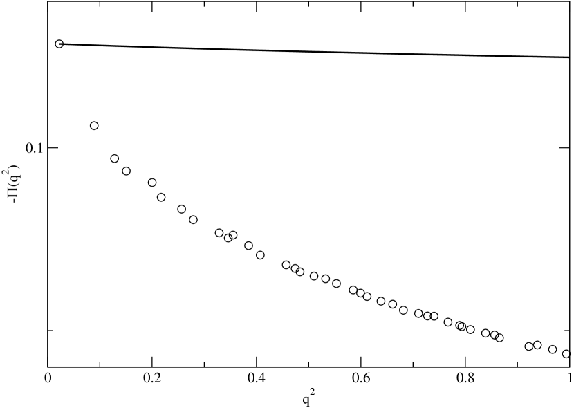
Figure 6: Comparison of Eq. (17) to the lattice vacuum polarization, where we have matched the two at the smallest value of $\hat{q}^{2}$ to fix the overall constant. The open circles are the datapoints (errors not shown) for the lightest quark mass used, $am_{l}=0.0031$. The solid line is the S$\chi$PT curve.

We find immediately that this expression does not describe the data at all. We can fix the overall constant $A$ by matching the data at the lowest value of the lattice momentum, $q^{2}=(2\pi/aT)^{2}\approx 0.0223$ GeV², for the largest lattice used in our study and use the values of the different meson masses from MILC_SPECTRUM . After fixing the overall constant there are no free parameters, and the resulting fit function and the lattice data for light quark mass $am_{l}=0.0031$ are shown in Figure 6. The slope for low $q^{2}$ is smaller by roughly two orders of magnitude in the fit function compared to the data. It is obvious that this cannot be a complete description of the low-energy physics for the photon vacuum polarization.

We can use our knowledge of the quenched simulations g-2_1 ; QCDSF to understand this. In the quenched case, the entire result for the vacuum polarization is described by a form dictated by vector particle intermediate states since they are absolutely stable in this case. We imagine that the vectors can also make a significant contribution to the photon vacuum polarization in the dynamical case, so we should include them in our calculation. Thus, the next section discusses how we incorporate vectors in S$\chi$PT.

IV Including vectors in S$\chi$PT as resonances

Including the lightest vector mesons such as the $\rho$ or the $\omega$ is more tricky than including the light pseudoscalars. Unlike the pions, the light vectors have no special role when discussing chiral symmetry. This is not an inherent problem, although there could be some model dependence which arises depending on how one includes the effects of the vectors. Here we use the formalism of Ecker, et al. in Ecker:1988te , treating the vectors as resonances in the effective field theory. This describes the vectors with antisymmetric Lorentz tensor fields, and not with Lorentz vector fields. With the correct free-field Lagrangian, this will enforce the correct number of degrees of freedom, and is useful when coupling the vectors to the photon Ecker:1988te . The particular form of the vector field should not alter the physics, as was discussed in Ref. Ecker:1989yg .

The octet of light vector mesons is an antisymmetric spin-1 field, $V_{\mu\nu}$, which is an $SU(12)$ matrix. The continuum free-field Lagrangian in Minkowski space is

$$\mathcal{L}_{v}=-\frac{1}{2}\textrm{Tr}\left[\partial^{\mu}V_{\mu\nu}\partial_{\rho}V^{\rho\nu}-\frac{1}{2}m_{V}^{2}V_{\mu\nu}V^{\mu\nu}\right]\ ,$$ (21)

where $m_{V}$ is the vector meson mass.

From the point of view of quark content, the vector fields have the same status as the light pseudoscalar fields. For example, a $\rho^{+}$ has the same light quark content as a $\pi^{+}$, although the relative spins of the constituent quarks are different. There is a fundamental difference from the point of view of chiral symmetry, in that the vectors do not have any special properties when the light quark masses vanish. What is important, however, is that the vectors and the pions have the same transformation property under the unbroken vector $SU(12)$ subgroup, as this is governed solely by the quark content. The primary difference is that we cannot determine the leading dependence of the vector mass $m_{V}$ on the quark masses from chiral symmetry alone, as we can for the pions.

As is standard in $\chi$PT, we expect the $SU(12)_{L}\!\times\!SU(12)_{R}$ chiral symmetry to spontaneously break down to the vector subgroup $SU(12)_{V}$. It is under this subgroup that the vector and pseudoscalar fields will have the same transformation property

$$\Sigma \to U_{V}\Sigma U_{V}^{\dagger}\ ,$$

$$V_{\mu\nu} \to U_{V}V_{\mu\nu}U_{V}^{\dagger}\ ,$$ (22)

where $U_{V}\in SU(12)_{V}$ is a constant vector transformation. With regard to the underlying chiral symmetry, any transformation which reduces to Eq. (IV) in the appropriate limit will lead to the same physics. A simple choice for the underlying transformations is made by defining $\sigma^{2}=\Sigma$, where under $SU(12)_{L}\!\times\!SU(12)_{R}$ we have

$$\sigma\to L\sigma U(x)^{\dagger}=U(x)\sigma R^{\dagger}\ .$$ (23)

$U(x)$ is an element of $SU(12)$, and since it depends on the pion fields, we see that it is position-dependent (the explicit form of $U(x)$ will not be needed). We can now define a transformation rule for the vector octet as

$$V_{\mu\nu}\to U(x)V_{\mu\nu}U(x)^{\dagger}\ .$$ (24)

When $SU(12)_{L}\!\times\!SU(12)_{R}\to SU(12)_{V}$, we set $U(x)=L=R=U_{V}$, and all the fields have the correct transformations under the unbroken vector subgroup.

The interaction terms to lowest order are given by

$$\mathcal{L}_{\rho}=\frac{f_{V}}{2\sqrt{2}}\textrm{Tr}\left(V_{\mu\nu}f_{+}^{\mu\nu}\right)+\frac{iG_{V}}{2\sqrt{2}}\textrm{Tr}\bigl{(}V_{\mu\nu}[\sigma^{\mu},\sigma^{\nu}]\bigr{)}\ ,$$ (25)

where $f_{V}$ and $G_{V}$ are real couplings ($f_{V}$ is the tree-level vector decay constant). We use the definitions

$$\sigma^{\mu} = i\sigma^{\dagger}D^{\mu}\Sigma\sigma^{\dagger}\ ,$$ (26)

$$f^{\mu\nu}_{+} = \sigma F^{\mu\nu}\sigma^{\dagger}+\sigma^{\dagger}F^{\mu\nu}\sigma\ ,$$ (27)

$$F^{\mu\nu} = eQ(\partial^{\mu}A^{\nu}-\partial^{\nu}A^{\mu})\ .$$ (28)

The second term in Eq. (25) will not affect the present calculation. An explicit form for the vector field is given by

$$V_{\mu\nu} = \left(\begin{matrix}\frac{1}{\sqrt{2}}\rho^{0}+\frac{1}{\sqrt{6}}\omega_{8}&\rho^{+}&K^{*+}\\ \rho^{-}&-\frac{1}{\sqrt{2}}\rho^{0}+\frac{1}{\sqrt{6}}\omega_{8}&K^{*0}\\ K^{*-}&\overline{K}^{*0}&-\frac{2}{\sqrt{6}}\omega_{8}\end{matrix}\right)_{\mu\nu}\ ,$$ (29)

where in this expression, each entry is a $4\!\times\!4$ matrix, corresponding to the 16 tastes of each vector meson.

We pause our discussion for a comment about the different tastes of a staggered vector meson. There are sixteen tastes, falling into eleven multiplets which are irreducible representations of the lattice symmetry group Golt_stag . Each of these irreps, in principle, will have different masses, but empirically the mass differences of the tastes are negligible. We use this fact to ignore these mass differences, to a first approximation, in the current analysis. Of course this does not imply that there can be no significant effects from taste-changing interactions among the vector particles in general, although we assume they give rise to errors which are smaller than the statistical and systematic errors already present in our calculation.

Finally, we should include terms in the vector part of the Lagrangian that could violate the taste symmetry, but we choose to neglect them for the following reasons. On one hand, taste violations arise through additional terms in the masses of the vectors (as happens with the pions), and these we neglect because empirically they are negligible. The other source of taste violations is additional terms that do not contribute to the tree-level masses but arise in one-loop calculations just as the flavor-neutral hairpins arise in pion masses and decay constants SCHPT ; FPI . We expect these contributions to be similar in size to the mass splittings (as in the pion sector), and thus negligible.

IV.1 Tree-level vector contribution

The tree-level calculation of the vacuum polarization involving the vectors is straightforward. We set $\sigma=1$ in the above expressions and find the vertices which couple the vectors to the photon. There are two two-point vertices: one where the photon couples to the $\rho^{0}$ and another where the photon couples to the $\omega_{8}$. The relevant diagram is shown in Figure 7, and from it, we get the following contribution to the photon vacuum polarization, after continuing the external momentum to Euclidean space,

$$\Pi^{\rm tree}_{V}(p^{2})=-\frac{\alpha}{4\pi}\frac{(4\pi f_{V})^{2}}{3}\left[\frac{3}{p^{2}+m^{2}_{V}}+\frac{1}{p^{2}+m^{2}_{V}}\right]=-\frac{\alpha}{4\pi}\frac{4}{3}\frac{(4\pi f_{V})^{2}}{p^{2}+m^{2}_{V}}\ .$$ (30)

In this expression, we have not included an explicit taste index on the vector mesons since we are neglecting the splittings between the various tastes. The full analysis requires making the transition from four to one tastes per flavor. By examining the Lagrangian above a similar analysis to the pion case leads to an overall factor of $1/16$ times a sum over the 16 tastes of vector mesons. Neglecting taste violations in the vector masses, the 16 degenerate contributions cancel the factor of $1/16$.

If we were to measure the decay constant as well as the vector masses on the lattice, then this expression has no free parameters. Notice that at this (lowest) order, the masses of both the $\rho^{0}$ and $\omega_{8}$ are the same, $m_{V}$. We can set this equal to the $\rho$ mass, and any discrepancies enter at ${\cal O}(p^{6})$ Ecker:1988te .

A quick analysis shows that for small momentum, the tree-level $\rho$ contribution dominates the one-loop pion contribution above. Expanding Eq. (30) around $p^{2}=0$, we get

$$\Pi^{\rm tree}_{V}(p^{2})=\Pi^{\rm tree}_{V}(0)+\frac{\alpha}{4\pi}\frac{4(4\pi f_{V})^{2}}{3}\frac{p^{2}}{m^{4}_{\rho^{0}}}+\mathcal{O}(p^{4})\ ,$$ (31)

while for the one-loop pion contribution we get

$$\Pi^{\rm 1-loop}_{1,\pi}(p^{2})=\Pi^{\rm 1-loop}_{1,\pi}(0)+\frac{\alpha}{4\pi}\frac{1}{16}\sum_{M,t}\frac{p^{2}}{30m^{2}_{M_{t}}}+\mathcal{O}(p^{4})\ .$$ (32)

To more easily compare these two expressions, let us first subtract off the zero momentum contribution, because it is the slope of the low-momentum region that we are interested in. Taking the ratio of these gives

$$\frac{\Pi^{\rm tree}_{V}(p^{2})-\Pi^{\rm tree}_{V}(0)}{\Pi_{\pi}(p^{2})-\Pi_{\pi}(0)}=\frac{640(4\pi f_{V})^{2}}{\displaystyle\sum_{M,t}\frac{m^{4}_{\rho^{0}}}{m^{2}_{M_{t}}}}\ .$$ (33)

Using a rough estimate for $f_{V}\approx 200$MeV Becirevic:2003pn , we see that only for very light pion masses will the pion contribution dominate. For the ensemble with the light quark mass $am_{l}=0.0062$, we see that

$$\sum_{M,t}\frac{1}{m^{2}_{M_{t}}}\approx 200{\rm GeV}^{-2},$$ (34)

and so for a vector mass of $\approx 800$MeV, Eq. (33) gives about 50. In the practical simulations we expect the vector contribution to dominate. Even at the physical masses in the continuum limit, this ratio is still roughly 10, so although the pion contribution becomes more important for lighter quark masses, the majority of the slope of the vacuum polarization comes from the vectors.

Although the contribution of Eq. (17) is much smaller that of the $\rho$, we will include it to determine the effects it has on the final fits. As such, we will have to include also the one-loop diagrams which involve the $\rho$ for consistency. This is done in the next section.

IV.2 One-loop terms with the $\rho$

The only diagram that will contribute here is shown in Figure 8 (there is a second, with the pion tadpole attached to the other vertex). There is also the possibility of a term arising as a self energy correction to the vector (so the vector line would have a pion loop inside). This has been evaluated (Eq. (28) of Rosell:2004mn ), but it is $\mathcal{O}(p^{4})$. Although this term is proportional to an unknown low energy constant that in principle could be rather large, to include it consistently would require us to include higher order terms from the pure pion sector. As such, it is consistent to neglect this piece.

A straightforward calculation gives the one-loop terms. Putting this together with the tree-level vector contribution we get the complete one-loop result for the vectors,

$$\Pi_{\rm vec}^{\rm 1-loop}(p^{2}) = -\frac{\alpha}{4\pi}\frac{(4\pi f_{V})^{2}}{3}\Biggl{\{}\frac{3}{p^{2}+m^{2}_{V}}\left[1-\frac{4}{(4\pi f)^{2}}\frac{1}{16}\sum_{t}\left[2\ell(m_{\pi_{t}}^{2})+\ell(m_{K_{t}}^{2})\right]\right]$$ (35)

$${}+\frac{1}{p^{2}+m^{2}_{V}}\left[1-\frac{12}{(4\pi f)^{2}}\frac{1}{16}\sum_{t}\ell(m_{K_{t}}^{2})\right]+\frac{C_{V}}{p^{2}+m_{V}^{2}}(3m_{\ell}+m_{s})\Biggr{\}}\ ,$$

where the usual chiral logarithm is

$$\ell(m^{2})=m^{2}\ln\left(\frac{m^{2}}{\Lambda^{2}}\right)\ ,$$ (36)

with $\Lambda$ the chiral scale, as before. The factors of $1/16$ arise in the same way as in the purely pion quark-flow analysis. As we are neglecting taste violations from the $\rho$, we can treat it as a taste singlet, and then the $\rho$-$2\pi$-photon vertex is identical in quark-level terms to the 2 photon-2 pion vertex. Thus, the quark-level diagrams are identical to those in Figure 5, with one of the photon lines taken to be a $\rho$ line. We again keep $m_{V}=m_{\rho^{0}}=m_{\omega}$, as the discrepancies are ${\cal O}(p^{6})$ and are still higher order than this expression Ecker:1988te . We have included an unknown coefficient, $C_{V}$, which would arise from analytic terms from the higher-order Lagrangian. This is necessary to cancel the scale dependence coming from the chiral logarithms.

We can see that this is roughly the same order of magnitude as the one-loop pion contribution, so if we were to include the one-loop pion expression in our final result, we would in principle need to include this. We do not explicitly include a constant term in Eq. (35), even though to this order it would be consistent to include such a term. Following the reasoning as in the pion sector, such a term would arise in the same manner. Since the full one-loop result would include Eqs. (17) and (35), this would amount to a change in the definition of the constant $A$ in terms of the underlying chiral parameters. As we are not explicitly writing down the higher-order terms in the Lagrangian in the $\rho$ sector, nor are we trying to extract the values of specific low-energy constants, we only need the mass and momentum dependence. Additionally, in the end this does not matter since to determine the muon $g\!-\!2$, we subtract off the value of the vacuum polarization at zero momentum, so any overall constant does not affect the physics. Note also, though, that the one-loop corrections in Eq. (35) could be absorbed into the definition of the parameter $f_{V}$, as there is no momentum dependence in these terms. We will discuss this further in the next section when we discuss the fits to the lattice data.

V Numerical Results

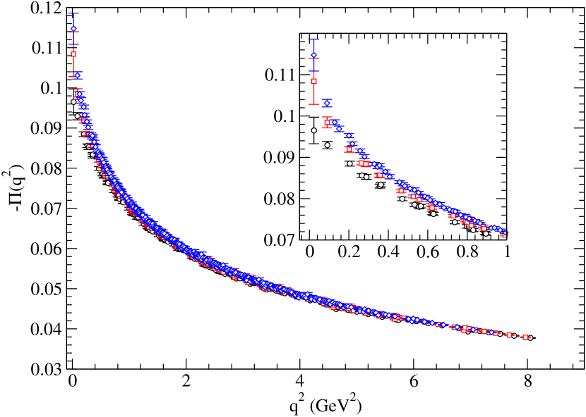
Figure 9: Minus the vacuum polarization for 2+1 flavors of quarks for each light quark mass studied in this work, 0.0031 (diamonds), 0.0062 (squares), and 0.0124 (circles). The insert shows a blow up of the important low $\hat{q}^{2}$ regime. The strange quark mass is fixed to 0.031 in each case.

We plot the results for the 2+1 flavor vacuum polarization as a function of $\hat{q}^{2}$ in Figure 9, including a close-up of the low-$\hat{q}^{2}$ region. As before g-2_1 ; g-2_2 ; g-2_3 , for larger $\hat{q}^{2}$, it is independent of quark mass, but as $\hat{q}^{2}\to 0$, there is a significant difference in the three plots. $\Pi(\hat{q}^{2})$ was computed using two quark propagator source times, 0 and 48, and results on the same lattice were averaged. We did not compute with both sources on every lattice, however, and strange and light valence quark propagators were calculated on overlapping but different subsets of each 2+1 flavor lattice ensemble (see Table 1). The statistical errors shown in Figure 9, and quoted throughout, come from a single elimination jackknife procedure. Because the numbers of strange and light valence quark propagators differ within the same $am_{l}=0.0031$ or 0.0062 ensemble, we adopted a jackknife procedure where each light or strange quark propagator calculation of $\Pi(\hat{q}^{2})$ is treated as a separate measurement, instead of the 2+1 flavor value of $\Pi(\hat{q}^{2})$. This is not expected to cause difficulty since the much heavier strange quark means the light and strange quark propagators computed on each lattice are roughly uncorrelated. Also, because of the electric charges, the light quark contribution is explicitly weighted five times more than the strange quark one. For the $am_{l}=0.0124$ ensemble, the jackknife error estimate for $\Pi(\hat{q}^{2})$ was calculated in the usual way. In all cases the errors were not significantly altered by increasing the jackknife block size to five, or by computing them using a simple binning procedure with bin size of ten configurations.

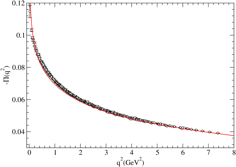
Figure 10: Comparison of the 2+1 flavor vacuum polarization computed using the lattice with 3-loop continuum perturbation theory in the $\overline{MS}$ scheme Chetyrkin:1996cf . The solid line is forced to match the lattice calculation at 2 GeV through a simple additive shift. $m_{l}=0.0031$ and $m_{s}=0.031$. The quark masses have been converted to the $\overline{MS}$ scheme using the matching factor in MILC_CHIRAL_FITS .

In Figures 10 and 11 we compare continuum three-loop perturbation theory Chetyrkin:1996cf with the lattice calculation of $-\Pi(q^{2})$ for $0\leq q^{2}\leq 8$ GeV² for $m_{l}=0.0031$ and 0.0124, respectively. The perturbative result is given in the $\overline{MS}$ scheme, and the bare quark mass has been matched using the renormalization factor given in StrangeMass . The results were forced to agree at $\mu=2$ GeV by a imposing a simple additive shift to the perturbation theory curve. The lattice results for $3\leq q^{2}\leq 8$ GeV² agree impressively with perturbation theory. For lower values of $q^{2}$ and $m_{l}=0.0031$, the lattice value increases faster until about 0.5 GeV² when the diverging perturbation theory result overtakes it again. For the heavier mass, the two results coincide until about 1 GeV² where the perturbative one again overtakes the non-perturbative one. This behavior with quark mass is mostly indicative of the variation with quark mass in the lattice results since the perturbation theory curve is insensitive to the light quark mass. This can also be seen from Figure 9; the two lattice results are clearly separated at 1 GeV². The above comparison is, of course, not unique. We could have matched the results at a value other than 2 GeV. Still, it is clear from Figures 10 and 11 that a large range of momentum values exist where perturbation theory is expected to be reliable, and the precise matching point will have little effect on the ultimate value of $a_{\mu}$. The matching point of 2 GeV is a natural choice, given the lattice scale in our study. This comparison is a non-trivial check of the lattice calculation of the vacuum polarization; in particular it indicates the correct number of physical quark degrees of freedom are accurately accounted for when using staggered fermions.

For the low energy regime, we have tried several different fits. In every case the fits are uncorrelated but performed under the single elimination jackknife procedure described above. Following previous calculations of the muon $g\!-\!2$ g-2_1 ; g-2_2 ; g-2_3 , we try various polynomial fits, up to quartic order in $\hat{q}^{2}$. The general form for these fits is

$$f(x)=\sum_{m=0}^{n}b_{m}x^{m}\,,$$ (37)

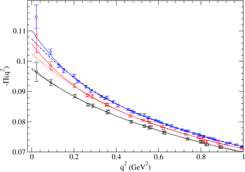
Figure 12: Cubic (dashed) and quartic (solid) fits to $-\Pi(\hat{q}^{2})$ for $am_{l}=0.0031$ (diamonds), $0.0062$ (squares), and 0.0124 (circles). The strange quark mass is fixed to 0.031 in each case.

with $x=\hat{q}^{2}$, and $n$ ranging from 1 to 4. We will refer to these fits individually as “Fit $n$.” For larger $n$ these fits have adequate values of $\chi^{2}$, but tend to undershoot the lowest momentum points except for $n=4$. For $n<3$, the fits have very poor $\chi^{2}$ and do not fit the low-$\hat{q}^{2}$ reqion well. In Figure 12, we display the cubic and quartic fits for each light quark mass. In Table 2, we show the results for the fitting parameters for cubic and quartic fits at each of the three different quark masses. Additionally, we use these results to determine the $\hat{q}^{2}<1$GeV² contribution to the leading hadronic contribution to the muon $g\!-\!2$, and give these results in Table 4. We will leave the discusion of these results to the next section.

More interesting are the fits using the S$\chi$PT vector resonance expressions for the vacuum polarization. We have performed three different fits:

Fit A:

Only the tree-level vector contribution given in Eq. (30).

Fit B:

Eqs. (17) and (30) which include the tree-level $\rho$ and the one-loop pion and kaon terms, but not the one-loop terms in Eq. (35).

Fit C:

The full one-loop expression, but absorbing the one-loop $\rho$ analytic term into $f_{V}$.

Note that the last two fits give identical results for $a_{\mu}$ since the pion and kaon logarithms and the NLO analytic term just serve to re-scale the (tree level) value of $f_{V}$ as the momentum dependence is identical to the tree-level expression. In other words, the overall factor multiplying the $(p^{2}+m_{V}^{2})^{-1}$ term stays the same, only the value of $f_{V}$ changes. Were we to be more precise, we would calculate the complete one-loop corrections to $f_{V}$ up to and including ${\cal O}(q^{4})$ terms and include these in the fitting functions. As our goal is to extract a value for the muon $g\!-\!2$, such a calculation, which for consistency also entails two loop diagrams in the pion sector, is beyond the scope of this paper.

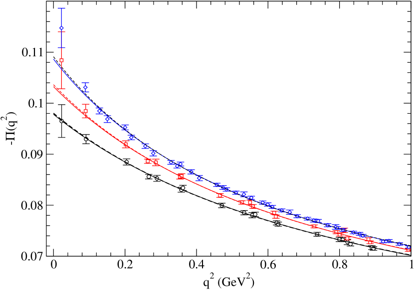
Figure 13: S$\chi$PT fits to $\Pi(\hat{q}^{2})$ for the three light masses, $am_{l}=0.0031$ (diamonds), $0.0062$ (squares), and 0.0124 (circles). The strange quark mass is fixed to 0.031 in each case. The solid lines correspond to Fit B, the dashed to Fit A, as described in the text.

The results from these fits with the maximum value of $q^{2}=1$ GeV² are shown in Table 3. The values for the decay constant change slightly from Fit A to Fit B when adding in the pions, and there is some tendency for the decay constant to decrease with quark mass. In other words, the one-loop corrections from the pion sector have only a small influence. Fit C shows the tree-level value of the decay constant changes dramatically due to the one-loop corrections in Eq. (35). The fits are shown along with the data in Figure 13. We take for the chiral scale $\Lambda=1$ GeV in Fits B and C.

The effect of decreasing the maximum value of $\hat{q}^{2}$ in the fit to 0.5 GeV² is small. The central value of $f_{V}$ changes by less than one percent, about two percent, and less than one percent for $m_{l}=0.0031$, 0.0062, and 0.0124, respectively. Raising the maximum to 1.5 GeV² induces larger changes, but the $\chi^{2}$ values of the fits are significantly worse. In all cases the vector masses are fixed to their nominal values from MILC_SPECTRUM . The polynomial fits are less stable, with very large errors for the smaller range, and significant undershooting of the data for the largest range. For these reasons we quote values of $a_{\mu}^{\rm HLO}$ using the “best” fit range, $0\leq q^{2}\leq 1.0$ GeV².

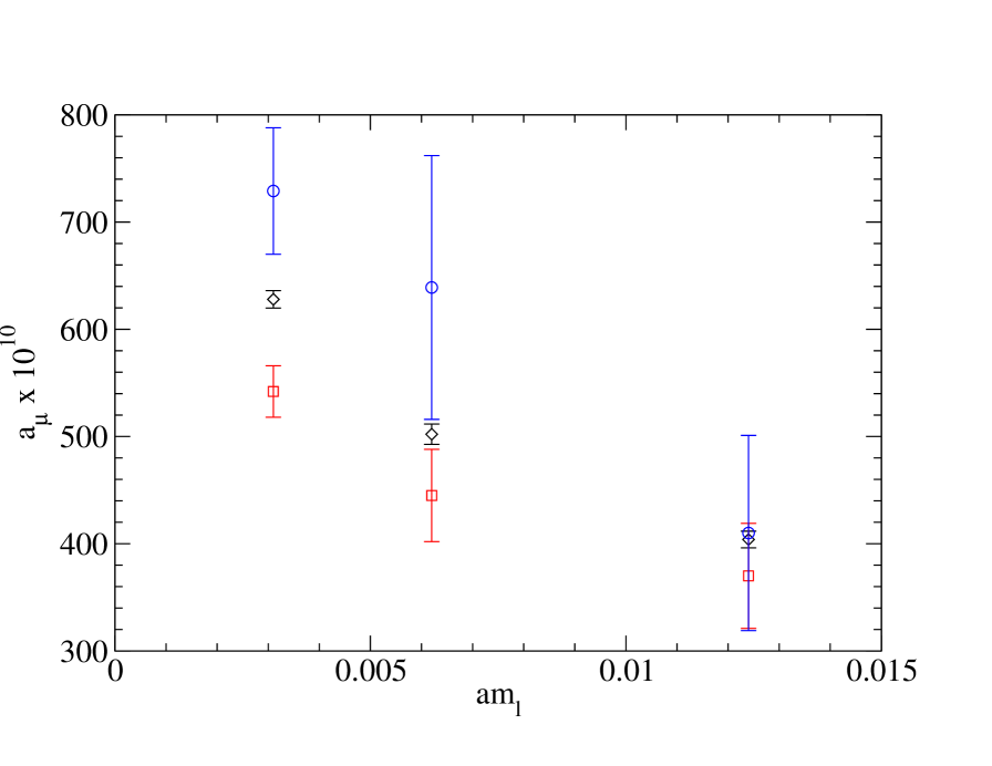
Figure 14: The hadronic contribution to the muon anomalous magnetic moment from polynomial and S$\chi$PT fits to the vacuum polarization. The statistical uncertainties for the cubic (squares) and quartic (circle) fits are much larger than the S$\chi$PT  one.

The values for $a_{\mu}^{\rm HLO}$ resulting from the above fits are listed in Table 4 and displayed in Figure 14, with only statistical errors shown. First, for the polynomial fits, we see a dramatic rise in $a_{\mu}^{\rm HLO}$ as we decrease the quark mass, and also as we increase the order of the polynomial; they are not stable in this sense. This is indicative of the calculation in general: the value of $a_{\mu}^{\rm HLO}$ is quite sensitive to the low momentum region, and hence the fit in this region, due to the nature of Eq. (3) and the smallness of the muon mass. The low $\hat{q}^{2}$ region is fit better as the order of the polynomial increases which increases the value of $a_{\mu}^{\rm HLO}$  but the errors on the fitted parameters increase such that the values for $a_{\mu}^{\rm HLO}$ also have large errors. Thus, it is preferable to use one of the physically motivated fitting functions. For Fits A and B, we note there is little difference in the final result for $a_{\mu}^{\rm HLO}$, as expected from the fit results themselves. As mentioned in the last section, there is no difference in $a_{\mu}^{\rm HLO}$ for Fits B and C since the one-loop corrections in Eq. (35) only rescale the tree-level value of $f_{V}$. The statistical errors on $a_{\mu}^{\rm HLO}$ for the S$\chi$PT fits are much smaller than the polynomial ones, so we use the former fits from now on to quote our best values.

From Figure 13 we see that the fits tend to undershoot the lattice calculation of $-\Pi(\hat{q}^{2})$ for the lowest momenta for the smallest two quark masses, though within roughly a standard deviation. As for the polynomial fits, even small changes in the fits in this region lead to large changes in $a_{\mu}^{\rm HLO}$. This undershooting behavior could represent real physics, or simply statistical and systematic errors. Certainly, the values of $-\Pi(\hat{q}^{2})$ at the smallest values of $\hat{q}^{2}$ are the most difficult to calculate, so the latter is more likely to be the case. The good fits obtained using chiral perturbation theory and the precisely measured meson masses from MILC_SPECTRUM , over a wide range of momentum, also back up this explanation. Still, the possibility that we have not accounted for an effect due to small quark mass and momentum remains, and must be further investigated in future calculations. In such calculations it is important to reduce the statistical error on these points as much as possible. One way to do this is to use a momentum source for each of the lowest momenta. This should have smaller errors than the point (-spilt) source used here, but is more complicated to implement and requires a separate propagator calculation for each momentum. Once the statistical errors on the very low $\hat{q}^{2}$ region are reduced, one can begin to investigate systematics to tell whether the excess is an actual physical effect (which could increase the value of $a_{\mu}^{\rm HLO}$ significantly).

In a similar vein, we should also check the numerics of our calculation. At the heart of the calculation is the quark propagator computation which is performed using the conjugate gradient algorithm to invert the lattice Dirac operator (matrix). The accuracy of the inversion is controlled by stopping the iterative solution found by the conjugate gradient algorithm when the norm of the so-called residual vector reaches some small size. The stopping criteria used here are given in Table 1 and are comparable in size to those used in other current simulations. They are also much smaller than the criteria used to generate the ensembles MILC_SPECTRUM . One test was run on a single $40^{3}$, $m_{l}=0.0031$, lattice to check whether the stopping criteria was adequate. We calculated the vacuum polarization using three stopping criteria, $10^{-5}$, $10^{-6}$, and $10^{-7}$, and compared the results. The difference in last two calculations was always less than 0.1 % except for two cases for the lowest momenta where the difference was still less than 1%, while the difference between the first two was always less than 1%, except for a handful of cases including one for the lowest momenta where the difference was neary 10%. Thus we chose to use a stopping criteria of $10^{-6}$ in this case (for all others we used $10^{-8}$), and we expect in all cases that the error in our results for the vacuum polarization due to a non-converged propagator solution is much smaller than the quoted statistical error.

The other possible problem with the numerics is the numerical precision of the calculation. In all cases the global sums in the quark propagator calculations were done in double precision and the rest of the calculation done in single (32-bit) precision, including the fourier transform of the vacuum polarization. This was also the procedure used in MILC_SPECTRUM , although in that calculation they did a comprehensive check for systematic errors arising from the use of single precision arithmetic (see Table VIII of MILC_SPECTRUM ). Any differences due to precision were much smaller than quoted statistical errors, or even statistical errors that might be achieved by a “reasonable lengthening” of their run.

Thus for now we attribute the excess of the vacuum polarization over the fit results at the lowest one or two momenta for the smallest two quark masses to statistics and possible systematics (but not numerics), and rely on the fits to chiral perturbation theory to provide an accurate determination of the anomalous magnetic moment. We also note that the chiral perturbation theory fits for all quark masses are very stable if we leave out the lowest two momenta, as would be expected from the relative size of the statistical errors on these points.

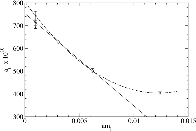
Figure 15: Linear and quadratic extrapolations (bursts) of the hadronic contribution to the muon anomalous magnetic moment to the physical point ($am_{l}\approx 0.001$). The left triangle is the currently accepted value, computed from the experimental cross-section for $e^{+}e^{-}\to$ hadrons g2REVIEW ; Davier:2004gb .

We need to extrapolate the values of $a_{\mu}^{\rm HLO}$ at fixed quark mass to the physical point (which, in lattice units, is a light mass of about $am_{l}\approx 0.001$ MILC_SPECTRUM ; MILC_CHIRAL_FITS ). There are several ways to do this. The simplest way is to extrapolate $a_{\mu}^{\rm HLO}$ in the light quark mass. This is shown in Figure 15, with two different “phenomenological” fits. One is a linear fit in the lightest two masses, and the other is a quadratic fit to all three. The value from the linear fit is

$$a_{\mu}^{{\rm HLO},q^{2}\leq 1}=(713\pm 15)\times 10^{-10}$$ (38)

while the quadratic gives

$$a_{\mu}^{{\rm HLO},q^{2}\leq 1}=(742\pm 21)\times 10^{-10},$$ (39)

where the errors are statistical. Of course, there is no guarantee that (other) non-linear behavior does not set in as the two pion threshold is crossed, which we discuss below.

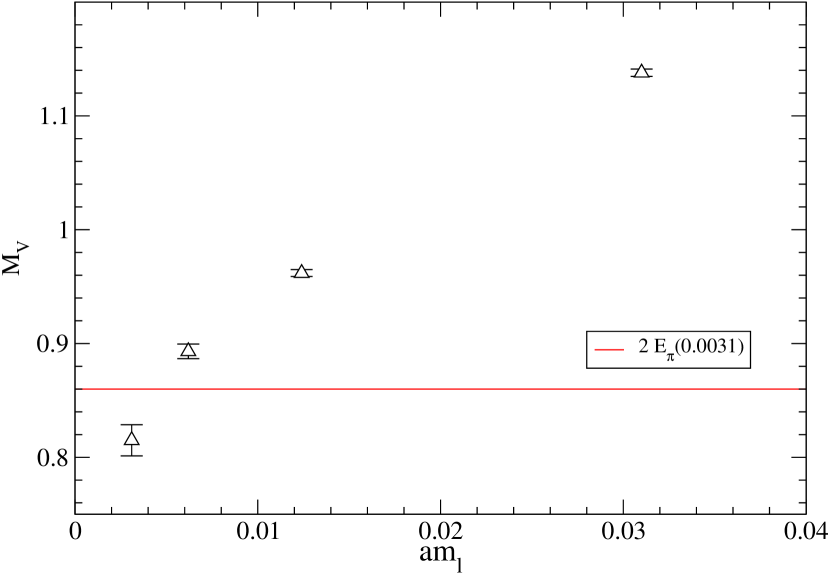
Figure 16: The vector meson mass (GeV). Non-linearity is visible for the lightest quark mass studied here, and perhaps even the second lightest mass. The horizontal line depicts the two pion energy for the largest lattice and smallest quark mass in our study. The mass values are from the MILC collaboration, MILC_SPECTRUM and DOUG ($am_{l}=0.0031$).

The more correct method to reach the physical value is to fit all the lattice data simultaneously, and extrapolate the vector decay constant and vector and pion masses to the physical light quark mass, with a single mass- and momentum- independent constant. The difficulty lies in the fact that such a fit requires computing the effects of the two pion threshold on the vector masses and decay constants, a clearly formidable task as the $\rho$ meson is unstable for physical quark masses. In our study, on the $40^{3}$ lattice with $am_{l}=0.0031$, the vector meson is just below the two pion threshold; however it shows clear non-linearity in the quark mass (see Figure 16). Lacking knowledge of two pion effects in chiral perturbation theory to the specified order at which we are working, we could instead simply develop smooth parameterizations of the masses (for example, see  Armour:2005mk ) and decay constants and use them in our chiral perturbation theory formulae. But such a complicated procedure is not likely to yield more accurate results from this study than the simple extrapolation we have used.

Using the continuum three-loop perturbation theory result matched to the $am_{l}=0.0031$ lattice calculation at 2 GeV as described above, we find

$$a_{\mu}^{{\rm HLO},q^{2}>1} = 6\times 10^{-10}$$ (40)

for the high energy region, $q^{2}>1$ GeV². There is some small error in this result made by running down to 1 GeV² instead of some higher value more compatible with the lattice calculation as seen in Figure 10. However, since the contribution to $a_{\mu}^{\rm HLO}$ is already so small starting at 1 GeV² and the difference between the perturbative curve and the lattice data is small even at 1 GeV², we did not bother to fit the lattice data with a stepwise procedure up to such a high momentum. Note also that the perturbative curve is insensitive to the value of the light quark mass, so we did not attempt to extrapolate this contribution to the physical light quark mass.

Adding the contributions from high and low momentum regions, the total value of the lowest order hadronic contribution to $g\!-\!2$ is

$$a_{\mu}^{\rm HLO}=(721\pm 15)\times 10^{-10}$$ (41)

for the linear fit, and

$$a_{\mu}^{\rm HLO}=(748\pm 21)\times 10^{-10},$$ (42)

for the quadratic. Our result is larger than the currently accepted theoretical numbers g2REVIEW ; Davier:2004gb , 692.4 (5.9) (2.4) $\times 10^{-10}$ and 711.0 (5.0)(0.8)(2.8) $\times 10^{-10}$ , which use only $e^{+}e^{-}$ data and include $\tau$ decay data, respectively. Considering our statistical errors and the systematic uncertainties described below, the calculations should be viewed as compatible for now.

VI Discussion

This calculation of $a_{\mu}^{\rm HLO}$ has focused on a detailed study of precisely fitting the lattice computed vacuum polarization to obtain the value of $g\!-\!2$ for several fixed quark masses. This has up to now only been done at a single lattice spacing, and as such, there are still discretization effects that could arise that we have not taken into account. Simulations using the coarser MILC lattices are underway AubinBlum , and new lattices with a smaller lattice spacing than the 0.086 fm used here are being generated by the MILC collaboration, so the continuum limit of the vacuum polarization can be taken. One way to gauge the size of the non-zero lattice spacing errors in our calculation, without actually repeating the calculation at another lattice spacing, is to use the naive continuum momenta $2\pi n/L$ everywhere in the analysis instead of the sin function ($2\sin{\pi n/L}$ appears in Ward-Takahashi identity so is the correct form to use). The resulting difference in $a_{\mu}^{\rm HLO}$ is within the statistical variation of the previous result. Other evidence that non-zero lattice spacing errors are under control is the agreement between the lattice calculation of $\Pi(\hat{q}^{2})$ and continuum perturbation theory, as already discussed in the previous section.

We also have not explicitly taken into account possible finite volume effects. The quark masses in these configurations are small enough to have small but not negligible finite volume corrections MILC_SPECTRUM ; MILC_CHIRAL_FITS . Most likely, however, these corrections are small compared with the statistical errors that exist in the data. In terms of our model used to fit the data, the dominant contribution is from a tree-level photon-$\rho$-photon diagram, where there will be no corrections coming from finite volume (other than the finite volume correction to the vector mass itself which is expected to be quite small). Finite volume corrections first appear in the one-loop diagrams and thus will be suppressed relative to the dominant contribution.

Another source of systematic error lies in the mismatch of the fixed value of the strange quark mass on these lattices and the physical strange quark mass which is actually about 10 percent smaller. Although we have assumed that the effect of this mismatch is negligible, this may not be the case. We can see from the lattice data that there is significant quark mass dependence for the vacuum polarization for low values of momenta. Note that correcting for this effect will tend to increase the value of $a_{\mu}^{\rm HLO}$.

Finally, as discussed already, the extrapolation to the physical light quark mass is not fully under control. Even though the extrapolations shown in Figure 15 appear sensible and are not large in the quark mass, the physical vector particles are unstable with non-zero widths, so these effects should be properly included in our analysis of resonance chiral perturbation theory. Such a calculation was beyond the scope of the present study as a consistent treatment of the pion and vector sectors entails higher order calculations.

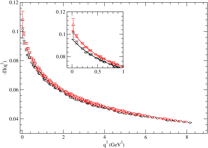
Figure 17: The vacuum polarization computed on the quenched ensemble (circles) compared to the 2+1 flavor result. The light quark mass in each case is 0.0062, and the quenched gauge coupling was tuned to match lattice spacings. The solid lines are fits to Eq. (30).

In this context it interesting to discuss the effects due to quenching since it is in this approximation that the vector particles are stable. In Figure 17 we show the quenched value of $-\Pi(q^{2})$ computed on an ensemble of lattices MILC_SPECTRUM with the same lattice spacing and volume as the $am_{l}=0.0062$, 2+1 flavor ensemble. The quenched and 2+1 flavor results agree at large $\hat{q}^{2}$, but a noticeable deficit occurs for the quenched case as $\hat{q}^{2}\to 0$. The resulting value of $a_{\mu}^{\rm HLO}$ is significantly lower (see Table 4), consistent with previous quenched calculationsg-2_1 ; QCDSF . Presumably this effect is caused by the sea quarks.

Even though the $\rho$ mass is always below the two pion threshold in our calculation, these two pion states contribute to the vacuum polarization, albeit with larger invariant mass, and on the lattice, a discrete spectrum. In our S$\chi$PT analysis two pion effects come only from the direct coupling to the photon; the two pion coupling to vector mesons is ${\cal O}(p^{4})$ and was not included. Because this coupling is higher order, we also expect that the effect of the non-zero width of the vector mesons on $a_{\mu}^{\rm HLO}$ is suppressed. The difference in the two cases is reflected, in the fits, through the vector mass itself which is significantly larger in the quenched case MILC_SPECTRUM and the decay constant which is also larger (see Table 3). A more complete understanding of these effects is wanting, and must await both simulations at smaller quark masses where the vectors are unstable and higher order calculations in chiral perturbation theory, some of which have been done already in continuum chiral perturbation theory Rosell:2004mn . We conclude this dicussion by emphasizing that there is a significant effect, clearly visible in the lattice calculations (see Figure 17), from unquenching which tends to increase the value of $a_{\mu}^{\rm HLO}$.

VII CONCLUSION

In this study we presented a value of the lowest order hadronic contribution to the muon anomalous magnetic moment computed in 2+1 flavor QCD. The statistical errors on our results at fixed light quark mass are small, possibly underestimated, and comparable with the errors on the accepted value of these contributions computed using the experimentally measured total cross sections for $e^{+}e^{-}$ annihilation to hadrons and tau lepton decay to hadronsg2REVIEW . The central value found by extrapolation to the physical light quark mass is slightly larger than this value, with statistical errors about 2-3 times larger. Within the systematic uncertainties in our calculation which were discussed in detail in the previous sections, the values should be seen as compatible.

First, there is some uncertainty in our fitting procedure. Polynomial fits require a high degree to fit the low momentum region of the vacuum polarization so that the statistical errors on the parameters become large. The results are also somewhat unstable to changes in the fit (momentum) range.

A more precise and stable fitting procedure was found by appealing to chiral perturbation theory, including lattice spacing effects. To our knowledge, this is the first time the hadronic vacuum polarization computed in chiral perturbation theory has been given in the literature. While the (staggered) chiral perturbation theory formula depends only on one (unknown) low energy constant and thus offers a useful fit function, we found that it does not represent the lattice calculation; to fit the data well requires the inclusion of the vector particles as well, through resonance chiral perturbation theory. This was already indicated by quenched calculations. The additional free parameter is the vector decay constant which shows modest quark mass dependence at tree level and large effects due to one-loop pion and kaon tadpole graphs. The coupling of the vector meson to two pions which contributes to both mass renormalization and the non-zero width of the $\rho$ meson gives rise to a one-loop graph which is however ${\cal O}(p^{4})$, and hence was not included in this work since a consistent treatment in the pion sector would require a two-loop computation. We also emphasize that a direct comparison to a “matched” quenched calculation showed a significant increase in the 2+1 flavor vacuum polarization at low momenta, presumably due to sea quark effects.

The vacuum polarization computed on the lattice was seen to be compatible with continuum weak-coupling perturbation theory over a wide range of momenta, between roughly 3 and 8 GeV². This indicates that lattice spacing errors may be under control in this study.

We have used the fits of the vacuum polarization to chiral perturbation theory to quote our final results. Remaining fitting uncertainties can be reduced in future calculations by reducing the statistical errors on the smallest momentum values of $\Pi(q^{2})$ and by including the ${\cal O}(p^{4})$ terms in the chiral perturbation theory analysis. The size of the statistical error can be further reduced by increasing the ensemble size, computing with momentum sources, and computing at smaller valence quark mass. These require modest increases of computational resources compared to those used here. Reducing the sea quark mass is obviously very costly, but not unforeseeable.

There are additional, as yet unquantified, systematic errors in our calculation, notably effects due to omission of disconnected quark diagrams giving rise to flavor singlet contributions, non-zero lattice spacing and unphysical quark masses. The latter were discussed at some length in the last section. The main point is that the two pion threshold may cause non-linearities in the light quark mass extrapolation which can be addressed by simulating below the threshold or, at least, by including higher order terms in the chiral expansion. It is also crucial to take the continuum limit and compute the vacuum polarization with different lattice fermions in light of the current understanding of the non-local nature of staggered fermions at non-zero lattice spacing. While these effects will be addressed in future calculations, the current study of the muon $g\!-\!2$ on the lattice in 2+1 flavor QCD appears quite encouraging.

Table 1: Parameters for the MILC lattices and propagator calculations in this study. “c.g. stop res.” is the stopping criterion, used for the residual vector in the conjugate gradient subroutine of the MILC code, for the valence quark propagator. The stopping criteria used to generate the lattices are given in Table I of MILC_SPECTRUM . In the “confs.” column total number of configurations are given for both propagator source time slices, $t=0$ and 48. $\beta=10/g^{2}$ is the bare gauge coupling for the tadpole-improved Symanzik gauge action used to generate the lattice ensembles MILC_SPECTRUM . The $\pi$, $K$, and vector meson masses used in this study were taken from MILC_SPECTRUM and DOUG ($am_{l}=0.0031$).

$a$ (fm)	size	$\beta$	$am_{l}$	$am_{s}$	$am_{\rm val}$	c.g. stop res.	confs.	$am_{\pi}$	$am_{K}$	$am_{V}$
0.086(2)	$28^{3}\times 96$	8.40	-	-	0.031	10-8	84/54
0.086(2)	$28^{3}\times 96$	8.40	-	-	0.0062	10-8	111/54
0.086(2)	$28^{3}\times 96$	7.11	0.0124	0.031	0.031	10-8	129/129
0.086(2)	$28^{3}\times 96$	7.11	0.0124	0.031	0.0124	10-8	129/129	0.20638 (18)	0.27209 (18)	0.4173 (13)
0.086(2)	$28^{3}\times 96$	7.09	0.0062	0.031	0.031	10-8	42
0.086(2)	$28^{3}\times 96$	7.09	0.0062	0.031	0.0062	10-8	249	0.14794 (19)	0.25319 (19)	0.3895 (28)
0.086(2)	$40^{3}\times 96$	7.08	0.0031	0.031	0.031	10-8	51/51
0.086(2)	$40^{3}\times 96$	7.08	0.0031	0.031	0.0031	10-6	161/153	0.10521 (8)	0.24175 (15)	0.357 (5)

Table 2: Fit parameters for the cubic and quartic polynomials for the 2+1 flavor value of $-\Pi(\hat{q}^{2})$. The fit range was taken to be $0\leq\hat{q}^{2}\leq 1$ GeV² in each case. The jackknife estimates of the errors are statistical only, and the $\chi^{2}$ values are from uncorrelated fits.

order	$am_{l}$	$b_{0}$	$b_{1}$	$b_{2}$	$b_{3}$	$b_{4}$	$\chi^{2}$/dof
3	0.0124	0.0972(14)	-0.051(7)	0.038(13)	-0.014(7)	—	3.5/16
4	0.0124	0.0978(20)	-0.058(14)	0.062(39)	-0.049(45)	0.017(19)	3.4/15
3	0.0062	0.1025 (14)	-0.0615 (63)	0.045 (10)	-0.015(5)	—	19.3/7
4	0.0062	0.1058 (27)	-0.092 (19)	0.137(48)	-0.124(51)	0.045(19)	16.3/16
3	0.0031	0.1075 (9)	-0.0754 (35)	0.0636 (54)	-0.0241 (27)	—	25.6/35
4	0.0031	0.1102(13)	-0.1044(89)	0.157(23)	-0.142(26)	0.051(10)	17.4/34

Table 3: Fit parameters for S$\chi$PT formulae for the 2+1 flavor value of $-\Pi(\hat{q}^{2})$. The first row is for the quenched case discussed in the text. The fit range was taken to be $0\leq\hat{q}^{2}\leq 1$ GeV². The jackknife estimates of the errors are statistical only, and the value of $\chi^{2}/$dof is from an uncorrelated fit. The meson masses were fixed to the values given in Table 1. The staggered meson mass splittings used in Fit B and Fit C (not shown) are found in MILC_SPECTRUM .

$am_{l}$	$f_{V}^{\rm FitA}$ (MeV)	$A^{\rm FitA}$	$\chi^{2}$/dof	$f_{V}^{\rm FitB}$ (MeV)	$A^{\rm FitB}$	$\chi^{2}$/dof	$f_{V}^{\rm FitC}$ (MeV)	$A^{\rm FitC}$	$\chi^{2}$/dof
0.0062	209.9 (2.0)	0.0410 (6)	23/18
0.0124	192.8 (1.8)	0.0445 (6)	4.4/18	188.6 (2.0)	0.0421 (7)	4.0/18	117.2 (1.2)	0.0420 (6)	4.0/18
0.0062	186.8 (1.7)	0.0453 (5)	18/19	181.6 (1.8)	0.0422 (5)	18 /19	115.7 (1.0)	0.0422 (5)	18/19
0.0031	175.4 (1.1)	0.0474 (3)	28/37	169.9 (1.1)	0.0436 (3)	25/37	111.5 (7)	0.0436 (3)	25/37

Table 4: Results for $a_{\mu}^{\rm HLO}\times 10^{10}$ for the various fits described in the text. Errors are jackknife estimates and statistical only. The quenched results correspond to light valence quark mass 0.0062 and strange valence quark mass 0.031.

Fit	quenched	$am_{l}=0.0124$	$am_{l}=0.0062$	$am_{l}=0.0031$
Poly 3	381 (63)	370(49)	445(43)	542(24)
Poly 4	588 (142)	410(91)	639(123)	729(59)
A	366.6 (7.0)	412.3 (7.8)	516.0 (9.5)	646.9 (8.1)
B		403.9 (7.8)	502.1 (9.5)	628.0 (8.1)
C		403.9 (7.8)	502.1 (9.5)	628.0 (8.1)

Figure 2: The two Wick contractions for the vacuum polarization. The dots are insertions of the vector current $J_{\mu}(x)$. Only the first has been calculated in this study.

Figure 3: The two one-loop diagrams contributing to the photon vacuum polarization in S$\chi$PT. The solid line can be either a charged pion or a charged kaon.

Figure 4: Quark-level vertex coming from the one-photon term in the Lagrangian. The solid lines are quarks.

Figure 5: Quark-level vertex coming from the two-photon term in the Lagrangian. As in Figure 4, the solid lines are quarks.

Figure 7: Tree-level diagram for a vector meson which contributes to the vacuum polarization. The double-line can be either the $\rho^{0}$ or the $\omega_{8}$.

Figure 8: The one-loop diagram involving the vector mesons. The solid line is either a pion or kaon, and the double solid line is the vector meson.

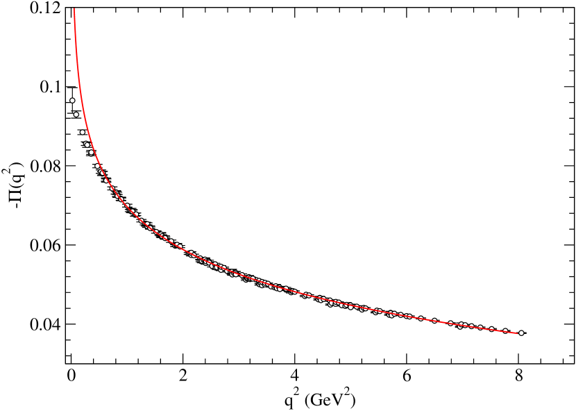
Figure 11: Same as Figure 10 but for $m_{l}=0.0124$.

References

- (1) Muon g-2, G. W. Bennett et al., Phys. Rev. D73, 072003 (2006), hep-ex/0602035.
- (2) Muon g-2, G. W. Bennett et al., Phys. Rev. Lett. 92, 161802 (2004), hep-ex/0401008.
- (3) M. Passera, J. Phys. G31, R75 (2005), hep-ph/0411168.
- (4) M. Davier and W. J. Marciano, Ann. Rev. Nucl. Part. Sci. 54, 115 (2004).
- (5) M. Hayakawa, T. Blum, T. Izubuchi, and N. Yamada, PoS LAT2005, 353 (2005), hep-lat/0509016.
- (6) M. Knecht, A. Nyffeler, M. Perrottet, and E. De Rafael, Phys. Rev. Lett. 88, 071802 (2002), hep-ph/0111059.
- (7) M. Hayakawa and T. Kinoshita, (2001), hep-ph/0112102.
- (8) J. Bijnens, E. Pallante, and J. Prades, Nucl. Phys. B626, 410 (2002), hep-ph/0112255.
- (9) K. Melnikov and A. Vainshtein, Phys. Rev. D70, 113006 (2004), hep-ph/0312226.
- (10) M. Ramsey-Musolf and M. B. Wise, Phys. Rev. Lett. 89, 041601 (2002), hep-ph/0201297.
- (11) J. Bijnens and J. Prades, (2007), hep-ph/0702170.
- (12) C. Bouchiat and L. Michel, J. Phys. Radium 22, 121 (1961).
- (13) M. Gourdin and E. De Rafael, Nucl. Phys. B10, 667 (1969).
- (14) T. Blum, Phys. Rev. Lett. 91, 052001 (2003), hep-lat/0212018.
- (15) QCDSF, M. Gockeler et al., Nucl. Phys. B688, 135 (2004), hep-lat/0312032.
- (16) T. Blum, Nucl. Phys. Proc. Suppl. 129, 904 (2004), hep-lat/0310064.
- (17) T. Blum, Nucl. Phys. Proc. Suppl. 140, 311 (2005), hep-lat/0411002.
- (18) C. Aubin and C. Bernard, Phys. Rev. D68, 034014 (2003), hep-lat/0304014.
- (19) C. Aubin and T. Blum, PoS LAT2005, 089 (2006), hep-lat/0509064.
- (20) Y. Shamir, (2006), hep-lat/0607007.
- (21) C. Bernard, M. Golterman, and Y. Shamir, Phys. Rev. D73, 114511 (2006), hep-lat/0604017.
- (22) C. Bernard, M. Golterman, Y. Shamir, and S. R. Sharpe, (2006), hep-lat/0603027.
- (23) C. Bernard, Phys. Rev. D73, 114503 (2006), hep-lat/0603011.
- (24) A. Hasenfratz and R. Hoffmann, Phys. Rev. D74, 014511 (2006), hep-lat/0604010.
- (25) M. Creutz, (2006), hep-lat/0603020.
- (26) S. R. Sharpe, PoS. LAT2006, 022 (2006), hep-lat/0610094.
- (27) S. Naik, Nucl. Phys. B316, 238 (1989).
- (28) MILC, K. Orginos and D. Toussaint, Phys. Rev. D59, 014501 (1999), hep-lat/9805009.
- (29) MILC, K. Orginos, D. Toussaint, and R. L. Sugar, Phys. Rev. D60, 054503 (1999), hep-lat/9903032.
- (30) G. P. Lepage, Phys. Rev. D59, 074502 (1999), hep-lat/9809157.
- (31) MILC, C. W. Bernard et al., Phys. Rev. D58, 014503 (1998), hep-lat/9712010.
- (32) C. Aubin et al., Phys. Rev. D70, 094505 (2004), hep-lat/0402030.
- (33) MILC, C. Aubin et al., Phys. Rev. D70, 114501 (2004), hep-lat/0407028.
- (34) J. Gasser and H. Leutwyler, Nucl. Phys. B250, 465 (1985).
- (35) S. R. Sharpe and R. S. Van de Water, Phys. Rev. D71, 114505 (2005), hep-lat/0409018.
- (36) C. Aubin and C. Bernard, (2005), hep-lat/0510088.
- (37) The MILC Collaboration, C. Bernard, Phys. Rev. D65, 054031 (2002), hep-lat/0111051.
- (38) G. Ecker, J. Gasser, A. Pich, and E. de Rafael, Nucl. Phys. B321, 311 (1989).
- (39) G. Ecker, J. Gasser, H. Leutwyler, A. Pich, and E. de Rafael, Phys. Lett. B223, 425 (1989).
- (40) M. F. L. Golterman, Nucl. Phys. B273, 663 (1986).
- (41) C. Aubin and C. Bernard, Phys. Rev. D68, 074011 (2003), hep-lat/0306026.
- (42) D. Becirevic, V. Lubicz, F. Mescia, and C. Tarantino, JHEP 05, 007 (2003), hep-lat/0301020.
- (43) I. Rosell, J. J. Sanz-Cillero, and A. Pich, JHEP 08, 042 (2004), hep-ph/0407240.
- (44) K. G. Chetyrkin, J. H. Kuhn, and M. Steinhauser, Nucl. Phys. B482, 213 (1996), hep-ph/9606230.
- (45) The HPQCD, MILC, and UKQCD Collaborations, C. Aubin et al., Phys. Rev. D70, 031504 (2004), hep-lat/0405022.
- (46) W. Armour, C. R. Allton, D. B. Leinweber, A. W. Thomas, and R. D. Young, J. Phys. G32, 971 (2006), hep-lat/0510078.
- (47) C. Aubin and T. Blum, in progress.
- (48) D. Toussaint, for the MILC collaboration, preliminary mass values for , private communication (2006).