Equation of state and QCD transition at finite temperature

Abstract

We calculate the equation of state in 2+1 flavor QCD at finite temperature with physical strange quark mass and almost physical light quark masses using lattices with temporal extent $N_{\tau}=8$. Calculations have been performed with two different improved staggered fermion actions, the asqtad and p4 actions. Overall, we find good agreement between results obtained with these two $O(a^{2})$ improved staggered fermion discretization schemes. A comparison with earlier calculations on coarser lattices is performed to quantify systematic errors in current studies of the equation of state. We also present results for observables that are sensitive to deconfining and chiral aspects of the QCD transition on $N_{\tau}=6$ and $8$ lattices. We find that deconfinement and chiral symmetry restoration happen in the same narrow temperature interval. In an Appendix we present a simple parametrization of the equation of state that can easily be used in hydrodynamic model calculations. In this parametrization we also incorporated an estimate of current uncertainties in the lattice calculations which arise from cutoff and quark mass effects. We estimate these systematic effects to be about $10$ MeV.

I Introduction

Determining the equation of state (EoS) of hot, strongly interacting matter is one of the major challenges of strong interaction physics. The QCD EoS provides a fundamental characterization of finite temperature QCD and is a critical input to the hydrodynamic modeling of the expansion of dense matter formed in heavy ion collisions. In particular, the interpretation of recent results from RHIC on jet quenching, hydrodynamic flow, and charmonium production RHIC rely on an accurate determination of the energy density and pressure as well as an understanding of both the deconfinement and chiral transitions.

For vanishing chemical potential, which is appropriate for experiments at RHIC and LHC, lattice calculations of the EoS aoki ; milc_eos ; rbcBIeos as well as the transition temperature milc04 ; tc06 ; aoki_Tc can be performed with an almost realistic quark mass spectrum. In addition, calculations at different values of the lattice cutoff allow for a systematic analysis of discretization errors and will soon lead to a controlled continuum extrapolation of the EoS with physical quark masses.

Studies of QCD thermodynamics are most advanced in lattice regularization schemes that use staggered fermions. In this case, improved actions have been developed that eliminate ${\cal O}(a^{2})$ discretization errors efficiently in the calculation of bulk thermodynamic observables at high temperature as well as at nonvanishing chemical potential Heller ; Hegde . At finite temperature, these cutoff effects are controlled by the temporal extent $N_{\tau}$ of the lattice as this fixes the cutoff in units of the temperature, $aT=1/N_{\tau}$. At tree level, which is relevant for the approach to the infinite temperature limit, the asqtad asqtad ; Orginos and p4 p4 ; Heller discretization schemes have been found to give rise to only small deviations from the asymptotic ideal gas limit already on lattices with temporal extent $N_{\tau}=6$. By $N_{\tau}=8$, the deviations from the continuum Stefan-Boltzmann value are at the 1% level Heller . At moderate values of the temperature, one expects that genuine nonperturbative effects will contribute to the cutoff dependence and, moreover, as the relevant degrees of freedom change from partonic at high temperature to hadronic at low temperature, other cutoff effects may become important. Most notably in the case of staggered fermions is the explicit breaking of staggered flavor (taste) symmetry that leads to ${\cal O}(a^{2})$ distortion of the hadron spectrum and will influence the thermodynamics in the confined phase.

To judge the importance of different effects that contribute to the cutoff dependence of thermodynamic observables, we have performed calculations with two different staggered fermion actions which deal with these systematic effects in different ways. The asqtad and p4 actions combined with a Symanzik improved gauge action eliminate ${\cal O}((aT)^{2})$ errors in thermodynamic observables at tree level. The asqtad action goes beyond tree-level improvement through the introduction of nonperturbatively determined tadpole coefficients milc_eos . In the gauge part of the action, this also means that in addition to the planar six link loop the nonplanar ‘parallelogram’ has been introduced. Furthermore, both actions use so-called fat links to reduce the influence of taste symmetry breaking terms inherent in staggered discretization schemes at nonzero values of the lattice spacing. The asqtad and p4 schemes also differ in the way fat-links are introduced. In the asqtad action, fat link coefficients have been adjusted so that tree-level coupling to all hard gluons has been suppressed without introducing further ${\cal O}(a^{2})$ errors. The p4 action, on the other hand, only uses a simple three-link staple for fattening.

In this paper, we report on detailed calculations of the thermodynamics of strongly interacting elementary particles performed in lattice-regularized QCD with a physical value of the strange quark mass and with two degenerate light quark masses being one tenth of the strange quark mass. To study the quark mass dependence of the thermodynamic quantities, we have also performed calculations at a larger value of the light quark mass corresponding to one fifth of the strange quark mass. Combining with past results on QCD thermodynamics at vanishing as well as nonvanishing values of the chemical potential on lattices with larger lattice spacing allows for an analysis of cutoff effects within both discretization schemes. In fact, a major obstacle to quantifying cutoff effects in studies of the QCD equation of state is that they arise from different sources which are strongly temperature dependent, and their relative importance changes with temperature. This makes it difficult to deal with them in a unique way and make a direct comparison between results obtained within different discretization schemes. It is, therefore, very important to understand and control systematic errors reliably.

In the next section, we start with a discussion of the basic setup for the calculation of the equation of state using the ${\cal O}(a^{2})$ improved asqtad and p4 actions. We proceed with a presentation of results for the trace anomaly that characterizes deviations from the conformal limit, in which the energy density ($\epsilon$) equals three times the pressure ($p$). In Sec. III, we give results on several bulk thermodynamic observables that can be derived from the trace anomaly $(\epsilon-3p)/T^{4}$ using standard thermodynamic relations. In Sec. IV, we analyze the temperature dependence of quark number susceptibilities, chiral condensates and the Polyakov loop expectation value and discuss in terms of them deconfining and symmetry restoring features of the QCD transition. We give our conclusions in Sec. V. Furthermore, we give a coherent discussion of calculations of the QCD equation of state with the asqtad and p4 actions in Appendix A. Appendix B summarizes results for renormalization constants needed to calculate the renormalized Polyakov loop expectation value with the asqtad action. In Appendix C we provide a parametrization for the equation of state suitable for application to hydrodynamic modeling of heavy ion collisions. All numerical results needed to calculate the bulk thermodynamic observables presented in this paper are given in Appendix D.

II Basic input into the calculation of the QCD Equation of State: Trace Anomaly

II.1 Calculational setup

This publication reports on a detailed study of the EoS of (2+1)-flavor QCD on lattices with temporal extent $N_{\tau}=8$. It extends earlier studies performed with the asqtad and p4 actions on lattices with temporal extent $N_{\tau}=4$ and $6$ milc_eos ; rbcBIeos . The calculational framework for the analysis of the equation of state, the thermodynamic quantities that need to be calculated and the dependence of various parameters that appear in the gauge and fermion actions on the gauge coupling $\beta=6/g^{2}$ has been discussed in these previous publications. It is, however, cumbersome to collect from the earlier publications all the information needed to follow the discussion given here, as the calculational set-up and the specific observables that need to be evaluated differ somewhat between the tadpole improved asqtad action milc_eos and the tree level improved p4 action rbcBIeos . In Appendix A we, therefore, give a coherent discussion of the various calculations performed with the asqtad and p4 actions, summarize the necessary theoretical background provided previously in the literature and unify the different notations and normalizations used in the past by different groups working with different staggered discretization schemes. In Appendix D, we give details of the simulation parameters and the statistics collected in each of these calculations.

Most of the finite temperature calculations presented here have been performed on lattices of size $32^{3}\times 8$ using the RHMC algorithm rhmc . We combine these results with earlier calculations at $N_{\tau}=6$. For the asqtad action we use both previous results using the inexact R algorithm milc_eos and new RHMC calculations on lattices of size $32^{3}\times 6$, while the p4 results have all been obtained using the RHMC algorithm. For each finite temperature calculation that entered our analysis of the equation of state, a corresponding ‘zero temperature’ calculation has been performed, mostly on lattices of size $32^{4}$, at the same value of the gauge coupling and for the same set of bare quark mass values, i.e., at the same value of the cutoff.

Following earlier calculations, we use a strange quark mass that is close to its physical value and two degenerate light quark masses that are chosen to be one tenth of the strange quark mass. This choice for the light quark masses corresponds to a light pseudo-scalar Goldstone mass of about $220$ MeV.

All calculations have been performed on a line of constant physics (LCP), i.e., as the temperature is increased the bare quark masses have been adjusted such that the values of hadron masses in physical units, evaluated at zero temperature, stay approximately constant. In practice, the LCP has been determined through the calculation of strange ($m_{K}$ or $m_{\bar{s}s}$) and nonstrange ($m_{\pi}$) meson masses in units of scales $r_{n}$ that characterize the shape of the static quark potential,

$$\left(r^{2}\frac{{\rm d}V_{\bar{q}q}(r)}{{\rm d}r}\right)_{r=r_{0}}=1.65\;\;,\;\;\left(r^{2}\frac{{\rm d}V_{\bar{q}q}(r)}{{\rm d}r}\right)_{r=r_{1}}=1.0\;\;.$$ (1)

A major concern when comparing calculations performed with two different discretizations of the QCD action is quantifying systematic errors. A natural way to make such a comparison is to simulate the two actions with a choice of parameters that give the same cutoff when expressed in physical units. The most extensive calculations done by us with the two actions are of the parameters $\hat{r}_{n}\equiv r_{n}/a$ that define the shape of the heavy quark potential. We therefore determine the cutoff scale and define a common temperature scale in units of $r_{n}$, i.e., $r_{n}T\equiv r_{n}/aN_{\tau}$. Note that for the comparison of results obtained with different actions, an accurate value of $r_{n}$ in physical units (1/MeV) is not necessary as only $r_{n}T$ is needed.

The ratio $r_{0}/r_{1}$ has been determined in the two discretization schemes consistently, as shown by the results $r_{0}/r_{1}=1.4636(60)$ (p4 rbcBIeos ) and $1.474(7)(18)$ (asqtad asqtad_pot ). We emphasize that these determinations of temperature scale based on parameters $\hat{r}_{0}$ and $\hat{r}_{1}$ were performed prior to the current combined analysis of thermodynamics with both the asqtad and p4 actions. Furthermore, this was done in completely independent calculations using data analysis strategies and fitting routines that have also been developed independently within the MILC milc_eos and RBC-Bielefeld rbcBIeos collaborations.

To determine scales $r_{0}$ and $r_{1}$ in physical units (MeV) we have related them to properties of the bottomonium spectrum. As our final input, we use the value $r_{0}=0.469(7)$ fm determined from the $\Upsilon(2S-1S)$ splitting lepage ; gray in calculations with the asqtad action. The same calculations show that the lattice scales from $r_{0}$ and $r_{1}$ are consistent with calculations of the pion and kaon decay constants as well as mass splittings between light hadronic states after extrapolations to the continuum limit and physical quark masses and agree with experimental results within errors of 3%. Note that all these observables, sometimes called gold-plated observables gold_plated , have been calculated within the same discretization scheme at identical values of the cutoff as used in the finite temperature studies reported here. This consistency gives us confidence in using scales extracted from the heavy quark potential for both extrapolating results to the continuum limit and for converting them to physical units. The scale $r_{0}T$ is shown on top of the figures.

In Table 1, we summarize the masses that characterize the LCP used for calculations with the p4 and asqtad actions. We find that the lines of constant physics are similar in both calculations, but differ in details. In particular, the strange pseudo-scalar mass on the LCP used for calculations with the asqtad action is 15% larger than the one used in the calculation with the p4-action. As the LCPs for asqtad and p4 actions had been fixed prior to this work in calculations on coarser lattices, we found it reasonable to stay with this convention rather than re-adjusting the choice of LCPs for this work. This makes the comparison of cutoff effects within a given discretization scheme easier. The difference in LCPs, however, should be kept in mind when comparing results obtained with different actions.

	p4-action	asqtad action
$m_{\bar{s}s}r_{0}$	1.59(5)	1.83(6)
$m_{\bar{s}s}/m_{K}$	1.33(1)	1.33(2)
$m_{\pi}/m_{K}$	0.435(2)	0.437(3)

Table 1: The strange pseudo-scalar mass $m_{\bar{s}s}\equiv\sqrt{2m_{K}^{2}-m_{\pi}^{2}}$ in units of $r_{0}$ and ratios of meson masses that characterize lines of constant physics for a fixed ratio of light and strange quark masses, $m_{s}/m_{q}=10$. The errors are not statistical. They represent a range of values over the lines of constant physics.

The statistics and details of the data needed to calculate the basic thermodynamic quantity, the trace anomaly, are summarized in Appendix D.

II.2 The trace anomaly

Along the LCP, i.e., for quark masses that are constant in physical units, and for sufficiently large volumes, temperature is the only intensive parameter controlling the thermodynamics. Consequently, in our calculations there is only one independent bulk thermodynamic observable that needs to be calculated. All other thermodynamic quantities are then obtained as appropriate derivatives of the QCD partition functions with respect to the temperature and by using standard thermodynamic relations.

The quantity most convenient to calculate on the lattice is the trace anomaly in units of the fourth power of the temperature $\Theta^{\mu\mu}/T^{4}$. This is given by the derivative of $p/T^{4}$ with respect to the temperature.

$$\frac{\Theta^{\mu\mu}(T)}{T^{4}}\equiv\frac{\epsilon-3p}{T^{4}}=T\frac{\partial}{\partial T}(p/T^{4})~{}~{}.$$ (2)

Since the pressure is given by the logarithm of the partition function, $p/T=V^{-1}\ln Z$, the calculation of the trace anomaly requires the evaluation of straightforward expectation values.

Using Eq. (2), the pressure is obtained by integrating $\Theta^{\mu\mu}/T^{5}$ over the temperature,

$$\frac{p(T)}{T^{4}}-\frac{p(T_{0})}{T_{0}^{4}}=\int_{T_{0}}^{T}{\rm d}T^{\prime}\frac{1}{T^{\prime 5}}\Theta^{\mu\mu}(T^{\prime})\;\;.$$ (3)

Here $T_{0}$ is an arbitrary temperature value that is usually chosen in the low temperature regime where the pressure and other thermodynamical quantities are suppressed exponentially by Boltzmann factors associated with the lightest hadronic states, i.e., the pions. We find it expedient to extrapolate to $T_{0}\equiv 0$, in which limit $p/T_{0}^{4}\equiv 0$. Energy ($\epsilon$) and entropy ($s=\epsilon+p$) densities are then obtained by combining results for $p/T^{4}$ and $(\epsilon-3p)/T^{4}$.

To calculate basic thermodynamic quantities such as energy density $\epsilon$, pressure $p$, and the trace anomaly, one needs to know several lattice $\beta$-functions along the LCP at $T=0$ on which our calculations have been performed. We determine these $\beta$-functions using the same parametrizations for the LCP as in the analysis of the EoS on lattices with temporal extent $N_{\tau}=6$ milc_eos ; rbcBIeos . Also, the determination of these $\beta$-functions in the nonperturbative regime is carried out on the same set of zero temperature lattices used to set the temperature scale. Further details are given in Appendix A.

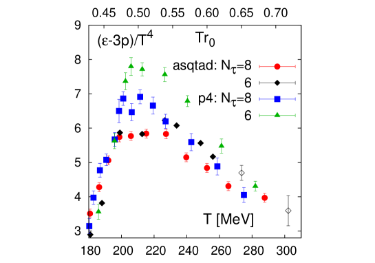
Figure 1: (color online) The trace anomaly $(\epsilon-3p)/T^{4}$ calculated on lattices with temporal extent $N_{\tau}=6,~{}8$. The upper x-axis shows the temperature scale in units of the scale parameter $r_{0}$ which has been determined in studies of the static quark potential. The lower x-axis gives the temperature in units of MeV, which has been obtained using for $r_{0}$ the value determined from the level splitting of bottomonium states, $r_{0}=0.469$ fm gray . The right hand figure shows the region around the maximum of $(\epsilon-3p)/T^{4}$, which also is the temperature region where results obtained with the two different discretization schemes show the largest differences. Open symbols for the $N_{\tau}=6$, asqtad data set denote data obtained with the R algorithm. All other data have been obtained with an RHMC algorithm.

In Fig. 1, we show results for $\Theta^{\mu\mu}/T^{4}$ obtained with both the asqtad and p4 actions. The new $N_{\tau}=8$ results have been obtained on lattices of size $32^{3}\times 8$ and the additional zero temperature calculations, needed to carry out the necessary vacuum subtractions, have been performed on $32^{4}$ lattices. The $N_{\tau}=6$ results for the p4 action shown for comparison are taken from rbcBIeos . For the asqtad action, new $N_{\tau}=6$ RHMC results obtained on $32^{3}\times 6$ lattices are shown using full symbols while earlier results obtained on $12^{3}\times 6$ lattices with the R algorithm milc_eos are shown using open symbols.

We find that the results with asqtad and p4 formulations are in good agreement. In particular, both actions yield consistent results in the low temperature range, in which $\Theta^{\mu\mu}/T^{4}$ rises rapidly, and at high temperature, $T\raise 1.29167pt\hbox{$>$\kern-7.5pt\raise-4.73611pt\hbox{$\sim$}}300$ MeV. This is also the case for the cutoff dependence in these two regimes. At intermediate temperatures, $200\;{\rm MeV}\raise 1.29167pt\hbox{$<$\kern-7.5pt\raise-4.73611pt\hbox{$\sim$}}T\raise 1.29167pt\hbox{$<$\kern-7.5pt\raise-4.73611pt\hbox{$\sim$}}300\;{\rm MeV}$, the two actions show differences (Fig. 1(right)). The maximum in $\Theta^{\mu\mu}/T^{4}$ is shallower for the asqtad action and shows a smaller cutoff dependence than results obtained with the p4 action.

As $(\epsilon-3p)/T^{4}$ is the basic input for the calculation of all other bulk thermodynamic observables, we discuss its structure in more detail in the following subsections.

II.2.1 The crossover region

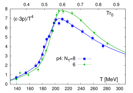
Figure 2: (color online) The trace anomaly calculated with the p4 (left) and asqtad (right) actions. Shown is a comparison of results obtained on lattices with temporal extent $N_{\tau}=6$ and $8$. The curves show interpolations discussed in the text. Open symbols for the $N_{\tau}=6$, asqtad data set denote data obtained with the R algorithm. All other data have been obtained with an RHMC algorithm.

In Fig. 2, we show results for the trace anomaly for both actions at $T<300$ MeV (about $1.5$ times the transition temperature) and for $N_{\tau}=6$ and 8 lattices. In the region $T\leq 170$ MeV, the curves shown are exponential fits. Above $T=170$ MeV, we divide the data into several intervals and perform quadratic interpolations. In each interval, these quadratic fits have been adjusted to match the value and slope at the boundary with the previous interval. These interpolating curves are then used to calculate the pressure and other thermodynamic quantities using Eqs. (2) and (3).

The differences between the $N_{\tau}=6$ and $8$ data in the transition region can well be accounted for by a shift of the $N_{\tau}=6$ data by about $5$ MeV towards smaller temperatures. This reflects the cutoff dependence of the transition temperature and may also subsume residual cutoff dependencies of the zero temperature observables used to determine the temperature scale in the transition region. As will become clearer later, we find a cutoff dependence of similar magnitude in other observables.

Such a global shift of scale for the $N_{\tau}=6$ data set also compensates for part of the cutoff dependence seen at higher temperatures. It thus is natural to expect that cutoff effects in $(\epsilon-3p)/T^{4}$ change sign at a temperature close to the peak in this quantity, which occurs at a temperature $T\raise 1.29167pt\hbox{$>$\kern-7.5pt\raise-4.73611pt\hbox{$\sim$}}200$ MeV. In the vicinity of this peak, we find the largest difference between results obtained with the two actions. The cutoff dependence in $(\epsilon-3p)/T^{4}$ with the p4 action is about twice as large as with the asqtad action, and the peak height is about 15% smaller with the asqtad action than with the p4 action.

It is of interest to compare how well the thermodynamics of the low temperature phase can be characterized by a resonance gas model. In the low temperature region, the hadron resonance gas has been observed pbm to give a good description of bulk thermodynamics. It also is quite successful in characterizing the thermal conditions met in heavy ion collisions at the chemical freeze-out temperature, i.e., at the temperature at which hadrons again form in the dense medium created in such collisions. In Fig. 3, we compare the results for $(\epsilon-3p)/T^{4}$ to predictions of the hadron resonance gas model pbm ,

$$\left(\frac{\epsilon-3p}{T^{4}}\right)_{low-T}=\sum_{m_{i}\leq m_{max}}\frac{d_{i}}{2\pi^{2}}\sum_{k=1}^{\infty}(-\eta_{i})^{k+1}\frac{1}{k}\left(\frac{m_{i}}{T}\right)^{3}K_{1}(km_{i}/T)\;,$$ (4)

where different particle species of mass $m_{i}$ have degeneracy factors $d_{i}$ and $\eta_{i}=-1(+1)$ for bosons (fermions). The particle masses have been taken from the particle data book databook . Data in Fig. 3 show the HRG model results including resonances up to $m_{max}=1.5$ GeV (lower curve) and $2.5$ GeV (upper curve). We find that the $N_{\tau}=8$ results are closer to the resonance gas model result and there is a tendency for the difference between the HRG model and lattice results to increase with decreasing temperature. This is not too surprising since the light meson sector is not well reproduced in current simulations. To quantify to what extent this reflects deviations from a simple resonance gas model or can be attributed to the violation of taste symmetry and/or the still too heavy Goldstone pion in our current analysis needs to be analyzed in more detail in the future. Qualitatively, the effects of staggered taste symmetry breaking and heavier quarks are to underestimate the energy density and pressure.

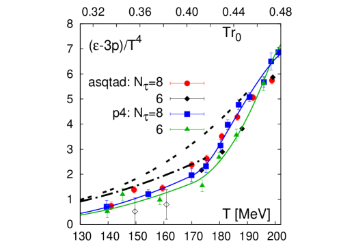
Figure 3: (color online) The trace anomaly at low temperatures calculated with the asqtad and p4 actions on lattices with temporal extent $N_{\tau}=6$ and $8$. Open symbols for the $N_{\tau}=6$, asqtad data set denote data obtained with the R algorithm. All other data have been obtained with an RHMC algorithm. Solid lines show interpolation curves for the p4 action discussed in the text. The dashed and dashed-dotted curves give the trace anomaly calculated in a hadron resonance gas model with two different cuts for the maximal mass, $m_{max}=1.5$ GeV (dashed-dotted) and $2.5$ GeV (dashed).

II.2.2 High temperature region

At high temperatures $(\epsilon-3p)/T^{4}$ will eventually approach zero in proportion to $g^{4}(T)\sim 1/\ln^{2}(T/\Lambda)$ Boyd . In the data shown in Fig. 4 for the temperature range accessible in our present analysis, i.e., $T\;\raise 1.29167pt\hbox{$<$\kern-7.5pt\raise-4.73611pt\hbox{$\sim$}}\;3.5T_{c}$, the variation of $(\epsilon-3p)/T^{4}$ with temperature is, however, significantly stronger. Following the analysis performed in rbcBIeos , we have fit the p4 data at $T>250$ MeV to the ansatz

$$\left(\frac{\epsilon-3p}{T^{4}}\right)_{high-T}=\frac{3}{4}b_{0}g^{4}+\frac{d_{2}}{T^{2}}+\frac{d_{4}}{T^{4}}\;,$$ (5)

where the first term gives the leading order perturbative result and the other terms parametrize nonperturbative corrections as inverse powers of $T^{2}$. We find that the $N_{\tau}=8$ data do not extend to high enough temperatures to control the first term in the ansatz given in Eq. (5). We thus performed fits to the p4 data sets with $g^{2}\equiv 0$ and the resulting fit parameters are summarized in Table 2. We find that these parameters are stable under variation of the fit range and show no significant cutoff dependence between $N_{\tau}=6$ and $8$ data. The fits for $T\geq 300$ MeV (Table 2) are shown in Fig. 4 together with the data obtained in the high temperature region. In our calculations with the asqtad action, we did not cover this high temperature regime with a sufficient number of data points to perform independent fits. However, in Appendix C we use a modified version of Eq. 5 to parametrize the equation of state for both p4 and asqtad for use in hydrodynamic codes. It is evident from Fig. 4 that results obtained with the asqtad action are in good agreement with the p4 results.

$N_{\tau}$	$d_{2}$ [GeV2]	$d_{4}$ [GeV4]	$\chi^{2}$/dof	$d_{2}$ [GeV2]	$d_{4}$ [GeV4]	$\chi^{2}$/dof
	$T\geq 300$ MeV			$T\geq 250$ MeV
4	0.101(6)	0.024(1)	1.23	0.137(15)	0.018(2)	7.38
6	0.26(5)	0.005(3)	1.16	0.23(2)	0.0086(16)	1.32
8	0.22(3)	0.008(4)	0.81	0.24(2)	0.0054(17)	0.66

Table 2: Parameters of fits to $(\epsilon-3p)/T^{4}$ in the region $T\geq 300$ MeV and $T\geq 250$ MeV using the ansatz given in Eq. (5) with $g^{2}\equiv 0$. In addition to fit results for $N_{\tau}=8$, we also reanalyzed the $N_{\tau}=6$ data of rbcBIeos setting the constant term in the ansatz to zero ($g^{2}\equiv 0$) and display again the fit result for the $N_{\tau}=4$ data given also in rbcBIeos . The 4th and 7th columns give $\chi^{2}$ per degree of freedom in the respective fit intervals.

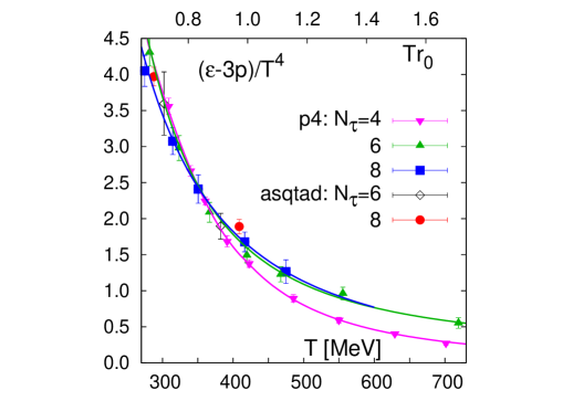
Figure 4: (color online) The trace anomaly at high temperatures calculated with the asqtad and p4 actions on lattices with temporal extent $N_{\tau}=6$ and $8$. For the p4 action we also show results obtained on lattices with temporal extent $N_{\tau}=4$ rbcBIeos . Open symbols for the $N_{\tau}=6$, asqtad data set denote data obtained with the R algorithm. All other data have been obtained with an RHMC algorithm. Solid curves show fits to the data based on Eq. (5). Fit parameters are given in Table 2.

II.3 Cutoff dependence of Gluon and Quark Condensates and continuum extrapolation of $\Theta^{\mu\mu}$

In this section, we want to discuss in more detail the various gluonic and fermionic contributions to the trace anomaly and use them to analyze the difference found in calculations performed with the asqtad and p4 actions. For nonvanishing quark masses, the trace anomaly receives contributions $\Theta_{F}^{\mu\mu}$ that are proportional to the quark mass and contain the quark condensates, and contributions $\Theta_{G}^{\mu\mu}$ that do not vanish in the chiral limit, i.e., from the gluon condensate,

$$\Theta^{\mu\mu}/T^{4}=\Theta^{\mu\mu}_{G}/T^{4}+\Theta^{\mu\mu}_{F}/T^{4}\;,$$ (6)

with $\Theta^{\mu\mu}_{G,F}$ defined in Eqs. (33) and (34) in Appendix A (for more details see rbcBIeos ).

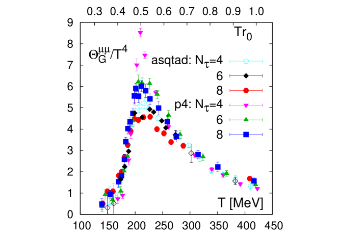
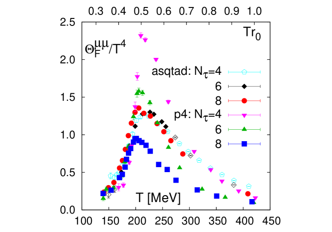
Figure 5: (color online) Gluon condensate and quark condensate contributions to the trace anomaly. Shown are results for the asqtad and p4 actions obtained on lattices of size $N_{\tau}=4,~{}6$ and $8$. Some results shown for the asqtad and p4 actions on lattices of size $N_{\tau}=4,~{}6$ have been taken from earlier calculations rbcBIeos ; milc_eos . Open symbols for the $N_{\tau}=4$ and $6$ asqtad data sets denote data obtained with the R algorithm. All other data have been obtained with an RHMC algorithm.

In Fig. 5, we show separately the two contributions $\Theta^{\mu\mu}_{G}/T^{4}$ and $\Theta^{\mu\mu}_{F}/T^{4}$. As seen already for $\Theta^{\mu\mu}/T^{4}$ cutoff effects are generally smaller for the asqtad action than for the p4 action. By comparing our results obtained on lattices with temporal extent $N_{\tau}=6$ and $8$, we estimate the overall cutoff dependence of $\Theta^{\mu\mu}/T^{4}$ in the vicinity of its maximum to be about 15% in calculations with the p4 action and only half that size in calculations with the asqtad action.

While for the latter action only the gluonic term $\Theta^{\mu\mu}_{G}/T^{4}$ shows some differences between the $N_{\tau}=6$ and 8 calculations, in the p4 case the cutoff effects mainly arise from the fermionic contribution $\Theta^{\mu\mu}_{F}/T^{4}$. Although they are large in this quantity, the quark condensates contribute less than 15% to the total trace anomaly. This contribution reduces to about 5% at $T\simeq 400$ MeV. We therefore conclude that at all values of the temperature, the trace anomaly is strongly dominated by the gluon condensate contribution which, in turn, receives contributions from the quark sector through interactions.

As pointed out in rbcBIeos , the cutoff dependence in $\Theta^{\mu\mu}_{F}/T^{4}$, seen for the p4 action, mainly arises from the structure of the nonperturbative $\beta$-functions that characterize the variation of bare quark masses along the LCP, i.e., $R_{m}$. This function appears as a multiplicative factor in the fermion contribution defined in Eq. (33) and approaches unity in the continuum limit. The influence of nonperturbative contributions to this prefactor thus is shifted to smaller temperatures as the lattice spacing is reduced, i.e., $N_{\tau}$ is increased, thereby reducing the cutoff dependence of $\Theta^{\mu\mu}_{F}/T^{4}$ at high temperatures. Comparing results for $N_{\tau}=6$ and $8$ one finds, indeed, that results for $\Theta^{\mu\mu}_{F}/T^{4}$ are more consistent for $T\raise 1.29167pt\hbox{$>$\kern-7.5pt\raise-4.73611pt\hbox{$\sim$}}300$ MeV. This suggest that the cutoff dependence should be drastically reduced in calculations on lattices with temporal extent $N_{\tau}=12$. To check this, we have performed calculations on $32^{3}\times 12$ lattices at 3 $\beta$-values. Our preliminary results indicate that results are indeed in good agreement with calculations on $N_{\tau}=8$ lattices performed at the same value of the temperature.

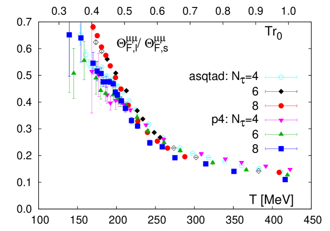
Figure 6: (color online) The ratio of light and strange quark contributions to the fermionic part of the trace anomaly on lattices with temporal extent $N_{\tau}=4$, 6, and $8$. Some results shown for the asqtad and p4 actions on lattices of size $N_{\tau}=4$, 6 have been taken from earlier calculations rbcBIeos ; milc_eos . Open symbols for the $N_{\tau}=4$ and $6$ asqtad data sets denote data obtained with the R algorithm. All other data have been obtained with an RHMC algorithm.

As can be seen in the right hand part of Fig. 5, results for $\Theta_{F}^{\mu\mu}/T^{4}$ obtained with the asqtad action are systematically larger than the $N_{\tau}=8$ results obtained with the p4 action. This is particularly evident in the high temperature region, $T\raise 1.29167pt\hbox{$>$\kern-7.5pt\raise-4.73611pt\hbox{$\sim$}}200$ MeV. At these values of the temperature $\Theta^{\mu\mu}_{F}/T^{4}$ is dominated by the contribution of the zero temperature strange quark condensate and the strange quark mass. The light quark contribution is suppressed by a factor $m_{l}/m_{s}$ and the thermal contributions are small, relative to the vacuum contributions, due to the disappearance of spontaneous symmetry at these temperatures. The difference in the p4 and asqtad results for $\Theta^{\mu\mu}_{F}/T^{4}$ thus can be traced back to the differences in the parametrization of the LCPs used in calculations with these two different actions. As pointed out in Sec. II.A, the strange pseudo-scalar $m_{\bar{s}s}$ is about 15% heavier on the asqtad LCP than on the p4 LCP. Through the GMOR relation, this is related to a larger value of the product $m_{s}\left\langle\bar{\psi}\psi\right\rangle_{s,0}$. The difference seen in Fig. 5, however, drops out in the relative contribution of light and strange quark condensates to $\Theta^{\mu\mu}_{F}/T^{4}$. In Fig. 6 we show the ratio

$$\frac{\Theta_{F,l}}{\Theta_{F,s}}=\frac{2m_{l}\left(\left\langle\bar{\psi}\psi\right\rangle_{l,0}-\left\langle\bar{\psi}\psi\right\rangle_{l,\tau}\right)}{m_{s}\left(\left\langle\bar{\psi}\psi\right\rangle_{s,0}-\left\langle\bar{\psi}\psi\right\rangle_{s,\tau}\right)}\;.$$ (7)

It is evident from this figure that results for $\displaystyle{\Theta_{F,l}/\Theta_{F,s}}$ agree quite well in calculations performed with the asqtad and p4 actions, respectively. This ratio shows much less cutoff dependence than the light and strange quark contributions separately. This is particularly evident in the case of the p4 action and supports the observation made before, that the cutoff dependence seen in that case mainly arise from the function $R_{m}$. This prefactor drops out in the ratio $\displaystyle{\Theta_{F,l}/\Theta_{F,s}}$.

As expected, the contribution of the light quark condensates is suppressed relative to the strange quark contribution because both terms are explicitly proportional to the light and strange quark masses, respectively. However, the naive expectation, $\displaystyle{\Theta_{F,l}/\Theta_{F,s}\leq 2m_{l}/m_{s}}$ only holds true for $T\raise 1.29167pt\hbox{$>$\kern-7.5pt\raise-4.73611pt\hbox{$\sim$}}300$ MeV, i.e., for temperatures larger than 1.5 times the transition temperature. In the transition region, the contribution arising from the light quark sector reaches about 50% of the strange quark contribution.

To summarize, we find that a straightforward ${\cal O}(a^{2})$ extrapolation of the trace anomaly to the continuum limit is not yet appropriate because the cutoff dependence arises from different sources which need to be controlled. Nonetheless, current $N_{\tau}=8$ data show that estimates for $\Theta^{\mu\mu}/T^{4}$ in the temperature regime [$200$ MeV, $300$ MeV] overestimate the continuum value by not more than 15% and less than 5% for $T>300$ MeV. Furthermore, our analysis of the quark contribution to the trace anomaly suggests that this contribution is most sensitive to a proper determination of the LCP that corresponds to physical quark mass values in the continuum limit. Our results suggest that it will be possible to control the cutoff effects in the entire high temperature regime $T\raise 1.29167pt\hbox{$>$\kern-7.5pt\raise-4.73611pt\hbox{$\sim$}}200$ MeV through calculations on lattices with temporal extent $N_{\tau}=12$.

III Thermodynamics: Pressure, energy and entropy density, velocity of sound

We calculate the pressure and energy density from the trace anomaly using Eqs. (2) and (3). To obtain the pressure from Eq. (3), we need to fix the starting point for the integration. In the past, this has been done by choosing a low temperature value ($T_{0}\simeq 100$ MeV) where the pressure is assumed to be sufficiently small to be set equal to zero due to the exponential Boltzmann suppression of the states. One could also use the hadron resonance gas value for the pressure at $T_{0}=100$ MeV as the starting point for the integration. The two HRG model fits in Fig. 3 show that at this temperature the pressure is insensitive to the exact value of the cutoff $m_{max}$. We have used both approaches as well as linear interpolations between the temperatures at which we calculated $\Theta^{\mu\mu}/T^{4}$ to estimate systematic errors arising in the calculation of the pressure. The actual results for $p/T^{4}$ and other thermodynamic observables shown in the following have been obtained by starting at $T_{0}=0$, where we set $p=0$, and integrating the fits to $\Theta^{\mu\mu}/T^{4}$ shown in Figs. 2 and 3. Differences arising from choosing $T_{0}\simeq 100$ MeV or using linear interpolations are small and are included in our estimate of systematic errors. In Fig. 7, we show our final results for $\epsilon/T^{4}$ and $3p/T^{4}$ obtained in this way. We reemphasize that $\Theta^{\mu\mu}/T^{4}$ is what we calculate at a number of temperature values along the LCP on the lattice, and all other quantities are obtained by using fits to this data and then exploiting thermodynamic relations.

Choosing $T_{0}=100$ MeV for the starting point of the integration, and adding the resonance gas pressure at this temperature to the lattice results gives a global shift of the pressure ($3p/T^{4}$) and energy density ($\epsilon/T^{4}$) curves by 0.8. This is indicated by the filled box in the upper right hand part of Fig. 7. Differences in the results that arise from the different integration schemes used to calculate the pressure are of similar magnitude. Typical error bars indicating the magnitude of this systematic error on $3p/T^{4}$ are shown in the right hand Fig. 7 at $T=275$ MeV and $T=540$ MeV. In this figure, we also compare results obtained on the $N_{\tau}=8$ lattices with the p4 and asqtad actions. The agreement between the two data sets is good in the entire temperature range that is common. This is a consequence of the good agreement for the trace anomaly, from which $\epsilon/T^{4}$ and $p/T^{4}$ are derived.

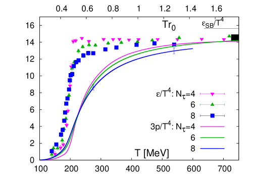
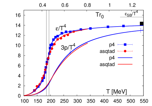
Figure 7: (color online) Energy density and three times the pressure calculated on lattices with temporal extent $N_{\tau}=4,~{}6$ rbcBIeos , and 8 using the p4 action (left). The right hand figure compares results obtained with the asqtad and p4 actions on the $N_{\tau}=8$ lattices. Crosses with error bars indicate the systematic error on the pressure that arises from different integration schemes as discussed in the text. The black bars at high temperatures indicate the systematic shift of data that would arise from matching to a hadron resonance gas at $T=100$ MeV. The band indicates the transition region $185\;{\rm MeV}<T<195\;{\rm MeV}$. It should be emphasized that these data have not been extrapolated to physical pion masses.

The same discussion applies to the entropy density, $s/T^{3}=(\epsilon+p)/T^{4}$, shown in Fig. 8 which is obtained by combining the results for energy density and pressure. The comparison of bulk thermodynamic observables ($p,\;\epsilon,\;s$) calculated on $N_{\tau}=8$ lattices yields a consistent picture for the p4 and asqtad actions. To quantify systematic differences, we consider the combination

$$\Delta O\equiv 2\frac{O_{1}-O_{2}}{O_{1}+O_{2}}\;,$$ (8)

where $O_{1}$ ($O_{2}$) are estimates with the p4 (asqtad) action. We find that the relative difference in the pressure $\Delta p$ for temperatures above the crossover region, $T\raise 1.29167pt\hbox{$>$\kern-7.5pt\raise-4.73611pt\hbox{$\sim$}}200$ MeV, is less than 5%. This is also the case for energy and entropy density for $T\raise 1.29167pt\hbox{$>$\kern-7.5pt\raise-4.73611pt\hbox{$\sim$}}230$ MeV with the maximal relative difference increasing to 10% at $T\simeq 200$ MeV. This is a consequence of the difference in the height of the peak in $(\epsilon-3p)/T^{4}$ as shown in Fig. 1. Estimates of systematic differences in the low temperature regime are less reliable as all observables become small rapidly. Nonetheless, the relative differences obtained using the interpolating curves shown in Figs. 7 and 8 are less than 15% for $T\raise 1.29167pt\hbox{$>$\kern-7.5pt\raise-4.73611pt\hbox{$\sim$}}150$ MeV. We also find that the cutoff errors between $aT=1/6$ and $1/8$ lattices are similar for the p4 action, i.e., about 15% at low temperatures and 5% for $T\raise 1.29167pt\hbox{$>$\kern-7.5pt\raise-4.73611pt\hbox{$\sim$}}200$ MeV. For calculations with the asqtad action, statistically significant cutoff dependence is seen only in the difference $(\epsilon-3p)/T^{4}$.

We conclude that cutoff effects in $p/T^{4},\;\epsilon/T^{4}$ and $s/T^{3}$ are under control in the high temperature regime $T\raise 1.29167pt\hbox{$>$\kern-7.5pt\raise-4.73611pt\hbox{$\sim$}}200$ MeV. Estimates of the continuum limit obtained by extrapolating data from $N_{\tau}=6$ and $8$ lattices differ from the values on $N_{\tau}=8$ lattices by at most 5%. These results imply that residual ${\cal O}(a^{2}g^{2})$ errors are small with both p4 and asqtad actions.

We note that at high temperatures the results for the pressure presented here are by 20% to 25% larger than those reported in aoki . These latter results have been obtained on lattices with temporal extent $N_{\tau}=4$ and $6$ using the stout-link action. As this action is not ${\cal O}(a^{2})$ improved, large cutoff effects show up at high temperatures. This is well known to happen in the infinite temperature ideal gas limit, where the cutoff corrections can be calculated analytically. For the stout-link action on the coarse $N_{\tau}=4$ and 6 lattices the lattice Stefan-Boltzmann limits are a factor $1.75$ and $1.51$ higher than the continuum value. In Ref. aoki it has been attempted to correct for these large cutoff effects by dividing the numerical simulation results at finite temperatures by these factors obtained in the infinite temperature limit. As is known from studies in pure $SU(N)$ gauge theories Boyd , this tends to over-estimate the actual cutoff dependence.

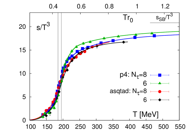
Figure 8: (color online) The entropy density obtained on lattices with temporal extent $N_{\tau}=6$ milc_eos ; rbcBIeos and $8$. The band indicates the transition region $185\;{\rm MeV}<T<195\;{\rm MeV}$.

Finally, we discuss the calculation of the velocity of sound from the basic bulk thermodynamic observables discussed above. The basic quantity is the ratio of pressure and energy density $p/\epsilon$ shown in Fig. 9, which is obtained from the ratio of the interpolating curves for $(\epsilon-3p)/T^{4}$ and $p/T^{4}$. On comparing results from $N_{\tau}=6$ and $8$ lattices with the p4 action, we note that a decrease in the maximal value of $(\epsilon-3p)/T^{4}$ with $N_{\tau}$ results in a weaker temperature dependence of $p/\epsilon$ at the dip (corresponding to the peak in the trace anomaly), somewhat larger values in the transition region and a slower rise with temperature after the dip.

From the interpolating curves, it is also straightforward to derive the velocity of sound,

$$c_{s}^{2}=\frac{{\rm d}p}{{\rm d}\epsilon}=\epsilon\frac{{\rm d}(p/\epsilon)}{{\rm d}\epsilon}+\frac{p}{\epsilon}\;.$$ (9)

Again, note that the velocity of sound is not an independent quantity but is fixed by the results for $\Theta^{\mu\mu}/T^{4}$. The determination of $c_{s}^{2}$ is sensitive to the details of the interpolation used to fit the data for $\Theta^{\mu\mu}/T^{4}$ obtained at a discrete set of temperature values. In fact, it was this sensitivity that motivated us to use a smooth curve with a continuous first derivative for the interpolation of $\Theta^{\mu\mu}/T^{4}$ in the entire temperature range. We consider the spread in the curves obtained from the p4 and asqtad calculations as indicative of the uncertainty in the current determination of the velocity of sound from the QCD equation of state (see also Appendix C).

Figure 9: (color online) Pressure divided by energy density ($p/\epsilon$) and the square of the velocity of sound ($c_{s}^{2}$) calculated on lattices with temporal extent $N_{\tau}=6$ (p4, rbcBIeos ) and $N_{\tau}=8$ using the p4 as well as the asqtad action. Lines without data points give the square of the velocity of sound calculated analytically from Eq. (9) using the interpolating curves for $\epsilon/T^{4}$ and $p/T^{4}$. The dashed-dotted line at low temperatures gives the result for $p/\epsilon$ from a hadron resonance gas (HRG) calculation using $m_{max}=2.5$ GeV.

IV Deconfinement and chiral symmetry restoration

In the previous sections, we discussed the thermodynamics of QCD with almost physical values of the quark masses. Data in Figs. 7 and 8 show that the transition from low to high temperatures occurs in a narrow temperature range: $T\in[180\;{\rm MeV},200\;{\rm MeV}]$. This represents a crossover and not a true phase transition caused by a singularity (nonanalyticity) in the QCD partition function. We expect such a singularity to exist in the chiral limit. For QCD with a physical value of the strange quark mass, it is not yet settled whether a true phase transition occurs only at strictly zero light quark masses ($m_{l}\equiv m_{crit}=0$) or at small but nonzero value ($m_{l}\equiv m_{crit}>0$). In the latter case, the second order phase transition will belong to the universality class of a three dimensional Ising model, while in the former case, it is expected to belong to the universality class of three dimensional, $O(4)$ symmetric spin models. For light quark masses $m_{l}\leq m_{crit}$ different observables that are defined through derivatives of the QCD partition function with respect to either the light quark mass or a temperature-like variable will give unambiguous signals for the occurrence and location of the phase transition. For $m_{l}>m_{crit}$, in the absence of a singularity, the determination of a pseudo-critical temperature that characterizes the crossover may depend on the observable used for its determination. It then becomes a quantitative question as to what extent different observables remain sensitive to the singular part of the free energy density $f_{sing}$ that controls thermodynamics in the vicinity of the phase transition temperature at $m_{crit}$. We write the free energy as

$$f=-\frac{T}{V}\log Z\equiv f_{sing}(t,\bar{m})+f_{reg}(T,m_{q})\;,$$ (10)

with the reduced mass and temperature variables,

$$\bar{m}\equiv|m_{l}-m_{crit}|\;\;{\rm and}\;\;t=\left|\frac{T-T_{c}}{T_{c}}\right|+c\left(\frac{\mu_{l}}{T_{c}}\right)^{2}\;.$$ (11)

Note that in the definition of the reduced temperature $t$, its dependence on the light quark chemical potential $\mu_{l}$ in the vicinity of the critical point $(t,\bar{m})\equiv(0,0)$ was taken into account. To leading order, the reduced temperature depends quadratically on $\mu_{l}$, while it is linear in the temperature itself.

Derivatives of the free energy with respect to quark masses define the light and strange quark chiral condensates,

$$\langle\bar{\psi}\psi\rangle_{q}=\frac{T}{V}\frac{\partial\ln Z}{\partial m_{q}}\;,\;\;q=l,\;s,$$ (12)

while derivatives with respect to temperature give the bulk thermodynamic quantities discussed in the previous sections. Here $m_{l}$ refers to one of the degenerate light up or down quark masses and the condensates defined in Eq. (12) are one-flavor condensates. The derivative of the chiral condensate with respect to the quark mass defines the chiral susceptibilities $\chi_{m,q}\sim\partial^{2}\ln Z/\partial m_{q}^{2}$. The divergence of $\chi_{m,q}$ at $T_{c}$ in the chiral limit is an unambiguous signal of the chiral phase transition. In addition, the fluctuations of Goldstone modes also induce divergences in the chiral limit for $T\leq T_{c}$ goldstone . Thus $\chi_{m,q}$ in the chiral limit is finite only for $T>T_{c}$.

In the vicinity of $T_{c}$, where thermodynamics is dominated by the singular part of the partition function, $n$ derivatives with respect to temperature $T$ are equivalent to $2n$ derivatives with respect to the light quark chemical potential. Second derivatives with respect to light and strange quark chemical potentials define quark number susceptibilities,

$$\frac{\chi_{q}}{T^{2}}=\frac{1}{VT^{3}}\frac{\partial^{2}\ln Z}{\partial(\mu_{q}/T)^{2}}\;,\;\;q=l,\;s\ .$$ (13)

Also, here $q=l$ refers to either the light up or down quark chemical potential, i.e., $\chi_{l}$ defines the fluctuations of a single light quark flavor. One therefore expects the quark number susceptibilities to exhibit a temperature dependence similar to that found for the energy density and the fourth order cumulant $c_{4}\sim\partial^{4}\ln Z/\partial(\mu_{q}/T)^{4}$ to behave like a specific heat $c_{V}$ rbcBIfluct . Also, the position of the peak in the fourth order cumulant is sensitive to the crossover region seen, for example, in the temperature dependence of $\epsilon/T^{4}$.

At $\bar{m}=0$, the temperature dependence of all the observables discussed above is sensitive to the location of $T_{c}$. Near $T_{c}$, their temperature dependence reflects the singular structure of the partition function,

$$\langle\bar{\psi}\psi\rangle_{l}\sim t^{\beta}\;({\rm for}\;T\leq T_{c}) \;\;,\;\; \frac{\chi_{l}}{T^{2}}\sim\frac{\epsilon}{T^{4}}\sim A_{\pm}t^{1-\alpha}+regular$$ (14)

$$\chi_{m,l}\sim t^{-\gamma}\;({\rm for}\;T\geq T_{c}) \;\;,\;\; c_{4}\sim c_{V}\sim A_{\pm}t^{-\alpha}+regular$$ (15)

where $\alpha,\;\beta,\;\gamma$ are critical exponents of the relevant universality class and $A_{\pm}$ are proportionality constants that may differ below and above $T_{c}$. The specific heat, and thus $c_{4}$, diverge at a generic second order phase transition, for example those in the Ising universality class, whereas these quantities only develop a pronounced peak in $O(N)$ symmetric models for which the critical exponent $\alpha$ exhibits unconventional behavior and is negative.

In the following subsections, we will focus on the temperature dependence of the chiral condensate and the quark number susceptibilities (Eq. (14)), which in the chiral limit probe the chiral symmetry restoring and deconfining features of the QCD phase transition. In particular, we will discuss the extent to which the temperature dependence of these quantities remains correlated away from $\bar{m}=0$.

IV.1 Deconfinement

The bulk thermodynamic observables $p/T^{4}$, $\epsilon/T^{4}$, and $s/T^{3}$ discussed in the previous sections are sensitive to the change from hadronic to quark-gluon degrees of freedom that occur during the QCD transition; they thus reflect the deconfining features of this transition. The rapid increase of the energy density, for instance, reflects the liberation of light quark degrees of freedom; the energy density increases from values close to that of a pion gas to almost the value of an ideal gas of massless quarks and gluons. In a similar vein, the temperature dependence of quark number susceptibilities gives information on thermal fluctuations of the degrees of freedom that carry a net number of light or strange quarks, i.e., $\chi_{q}\sim\langle N_{q}^{2}\rangle$, with $N_{q}$ denoting the net number of quarks carrying the charge $q$. Quark number susceptibilities change rapidly in the transition region as the carriers of charge, strangeness or baryon number are heavy hadrons at low temperatures but much lighter quarks at high temperatures. In the continuum and infinite temperature limit, these susceptibilities approach the value for an ideal massless one flavor quark gas, i.e., $\lim_{T\rightarrow\infty}\chi_{q}/T^{2}=1$. At low temperatures, however, they reflect the fluctuations of hadrons carrying net light quark (up or down) or strangeness quantum numbers. In the zero temperature limit, $\chi_{s}/T^{2}$ receives contributions only from the lightest hadronic state that carries strangeness, $\chi_{s}/T^{2}\sim\exp(-m_{K}/T)$, while $\chi_{l}/T^{2}$ is sensitive to pions, $\chi_{l}/T^{2}\sim\exp(-m_{\pi}/T)$. Note that $\chi_{l}/T^{2}$ is directly sensitive to the singular structure of the QCD partition function in the chiral limit.

In Fig. 10, we show results for the temperature dependence of the light and strange quark number susceptibilities. For the ${\cal O}(a^{2})$ improved p4 and asqtad actions, deviations from the continuum result are already small in calculations on lattices with temporal extent $N_{\tau}=8$. The continuum ideal gas value, $\chi_{q}/T^{2}=1$, is thus a good guide for the expected behavior of $\chi_{l}/T^{2}$ in the high temperature limit. As can be seen from the figure, cutoff effects are indeed small at high temperature. In fact, we observe that above the transition, in particular for temperatures up to about 1.5 times the transition temperature, differences between results obtained with the asqtad and p4 actions are larger than the cutoff effects seen for each of these actions separately. This is similar to what has been found in calculations of the energy density discussed in the previous section.

The rise of $\chi_{l}/T^{2}$ in the transition region is compatible with the rapid rise of the energy density. The strange quark number susceptibility, on the other hand, rises more slowly in the transition region. The astonishingly strong correlation between energy density and light quark number susceptibility is evident from the ratio $\epsilon/(T^{2}\chi_{l})$ shown in Fig. 11(left). The ratio $\epsilon/(T^{2}\chi_{l})$ varies in the transition region by about 15%. This is in contrast to the ratio $\epsilon/(T^{2}\chi_{s})$ which starts to increase with decreasing temperature already at $T\simeq 250$ MeV and rises by about 50% in the transition region. In fact, unlike $\epsilon/(T^{2}\chi_{l})$, the ratio $\epsilon/(T^{2}\chi_{s})$ will diverge in the zero temperature limit as $\chi_{s}$ goes to zero faster than $\epsilon$ since it is not sensitive to the light quark degrees of freedom that contribute to the energy density. This lack of sensitivity of $\chi_{s}/T^{2}$ to the singular structure of the QCD partition function suggests that $\chi_{s}/T^{2}$ is not a good quantity to use to define the pseudo-critical temperature.

The difference in light and strange quark masses plays an important role in the overall magnitude of quark number fluctuations up to almost twice the transition temperature. This is seen in Fig. 11(right), where we show the ratio $\chi_{s}/\chi_{l}$. At $T\raise 1.29167pt\hbox{$>$\kern-7.5pt\raise-4.73611pt\hbox{$\sim$}}300$ MeV the ratio $\chi_{s}/\chi_{l}$ comes close to the infinite temperature ideal gas value $\chi_{s}/\chi_{l}=1$. Deviations from this may be understood as a thermal effect that arises even in a noninteracting gas from just the differences in quark masses. However, as has been discussed in rbcBIfluct , this clearly is not possible in the transition region, $200~{}{\rm MeV}\raise 1.29167pt\hbox{$<$\kern-7.5pt\raise-4.73611pt\hbox{$\sim$}}T\raise 1.29167pt\hbox{$<$\kern-7.5pt\raise-4.73611pt\hbox{$\sim$}}300~{}{\rm MeV}$ where, upon cooling, strangeness fluctuations decrease strongly relative to light quark fluctuations as $T$ decreases. At the transition temperature, $\chi_{s}/\chi_{l}$ is only about $1/2$ and has the tendency to go over smoothly into values extracted from the HRG model. In the low temperature hadronic region, the ratio $\chi_{s}/\chi_{l}$ drops exponentially as strangeness fluctuations are predominantly carried by heavy kaons whereas the light quark fluctuations are carried by light pions.

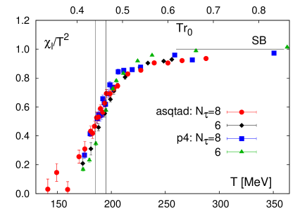
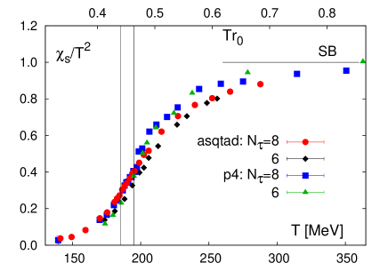
Figure 10: (color online) The light (left) and strange (right) quark number susceptibilities calculated on lattices with temporal extent $N_{\tau}=6$ and $8$. The $N_{\tau}=6$ results for the p4 action are taken from rbcBIeos . The band corresponds to a temperature interval $185\;{\rm MeV}\leq T\leq 195\;{\rm MeV}$.

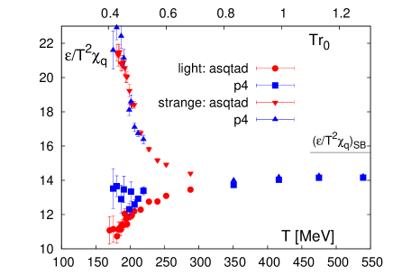
Figure 11: (color online) The ratio of energy density and quark number susceptibilities (left) and the ratio of strange and light quark number susceptibilities (right) calculated on lattices with temporal extent $N_{\tau}=8$. For the energy densities the interpolating curves shown in Fig. 7 have been used. Curves in the right hand figure show results for a hadron resonance gas including resonance up to $m_{max}=1.5$ GeV (upper branch) and $2.5$ GeV (lower branch), respectively.

IV.2 Chiral symmetry restoration

In the limit of vanishing quark masses, the chiral condensate $\langle\bar{\psi}\psi\rangle_{l}$ introduced in Eq. (12) is an order parameter for spontaneous symmetry breaking; it stays nonzero at low temperature and vanishes above a critical temperature $T_{c}$. Chiral symmetry is broken spontaneously for $T<T_{c}$.

At zero quark mass, the chiral condensate needs to be renormalized only multiplicatively. At nonzero values of the quark mass, an additional renormalization is necessary to eliminate singularities that are proportional to $m_{q}/a^{2}$. An appropriate observable that takes care of the additive renormalizations is obtained by subtracting a fraction, proportional to $m_{l}/m_{s}$, of the strange quark condensate from the light quark condensate. To remove the multiplicative renormalization factor we divide this difference at finite temperature by the corresponding zero temperature difference, calculated at the same value of the lattice cutoff, $i.e.$,

$$\Delta_{l,s}(T)=\frac{\langle\bar{\psi}\psi\rangle_{l,T}-\frac{m_{l}}{m_{s}}\langle\bar{\psi}\psi\rangle_{s,T}}{\langle\bar{\psi}\psi\rangle_{l,0}-\frac{m_{l}}{m_{s}}\langle\bar{\psi}\psi\rangle_{s,0}}\;.$$ (16)

This observable has a sensible chiral limit and is an order parameter for chiral symmetry breaking. It is unity at low temperatures and vanishes at $T_{c}$ for $m_{l}=0$. For the quark mass values used in our study of bulk thermodynamics, i.e., $m_{l}=0.1m_{s}$, its temperature dependence is shown in Fig. 12. It is evident that $\Delta_{l,s}(T)$ varies rapidly in the same temperature range as the bulk thermodynamic observables and the light quark number susceptibility. Based on this agreement we conclude that the onset of liberation of light quark and gluon degrees of freedom (deconfinement) and chiral symmetry restoration occur in the same temperature range in QCD with almost physical values of the quark masses, i.e., in a region of the QCD phase diagram where the transition is not a true phase transition but rather a rapid crossover.

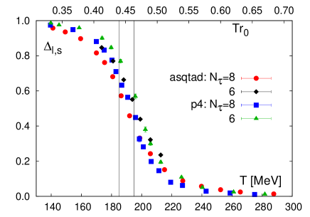
Figure 12: (color online) The subtracted chiral condensate normalized to the corresponding zero temperature value (right). In the right hand figure data for $N_{\tau}=6$ calculations have been shifted by $-7$ MeV (asqtad) and $-5$ MeV (p4),

Cutoff effects in the chiral condensate as well as in bulk thermodynamic observables are visible when comparing calculations performed with a given action at two different values of the lattice cutoff, e.g., $N_{\tau}=6$ and $8$. These cutoff effects can to a large extent be absorbed in a common shift of the temperature scale. This is easily seen by comparing the left and right panels in Fig. 12. A global shift of the temperature scale used for the $N_{\tau}=6$ data sets by $5$ MeV for the p4 and by $7$ MeV for the asqtad action makes the $N_{\tau}=6$ and $8$ data sets coincide almost perfectly. This is similar in magnitude to the cutoff dependence observed in $(\epsilon-3p)/T^{4}$ and again seems to reflect the cutoff dependence of the transition temperature as well as residual cutoff dependencies of the zero temperature observables used to determine the temperature scale.

As can be seen from Fig. 12(right), even after the shift of temperature scales the chiral condensates calculated with asqtad and p4 actions show significant differences. This reflects cutoff effects arising from the use of different discretization schemes and to some extent is also due to the somewhat different physical quark mass values on the LCPs for the asqtad and p4 actions. The differences are most significant at low temperatures where the lattice spacing is quite large. Here, cutoff effects that arise from the explicit breaking of flavor symmetry in the staggered fermion formulations may become important. At temperatures larger than the crossover temperature, the chiral condensate obtained from calculations with the asqtad action is systematically larger than that obtained with the p4 action. This is consistent with the fact that the quark masses used on the asqtad LCP are somewhat larger than those on the p4 LCP.

We note that at finite temperatures the chiral condensate as well as $\Delta_{l,s}(T)$ are quite sensitive to the quark mass. In the chiral symmetry broken phase, in both cases the leading order quark mass correction is proportional to the square root of the light quark mass goldstone . Small differences in the actual quark mass values used in p4 and asqtad calculations on lattices with temporal extent $N_{\tau}=6$ and $8$ will thus be enhanced in the transition region. This makes it important to have good control of the line of constant physics. We will discuss the quark mass dependence of the chiral condensate and quark number susceptibilities as well as the cutoff dependence of pseudo-critical temperatures extracted from them in more detail in a forthcoming publication hotTc .

IV.3 The Polyakov loop

The logarithm of the Polyakov loop is related to the change in free energy induced by a static quark source. It is a genuine order parameter for deconfinement only for the pure gauge theory, $i.e.$, all quark masses taken to infinity. At finite quark masses it is nonzero at all values of the temperature but changes rapidly at the transition. The Polyakov loop operator is not present in the QCD action but can be added to it as an external source. Its expectation value is then given by the derivative of the logarithm of the modified partition function with respect to the corresponding coupling, evaluated at zero coupling. As far as we know, the Polyakov loop is not directly sensitive to the singular structure of the partition function in the chiral limit. Therefore, its susceptibility will not diverge at $\bar{m}=0$ nor is its slope in the transition region related to any of the critical exponents of the chiral transition. Nonetheless, the Polyakov loop is observed to vary rapidly in the transition region indicating that the screening of static quarks suddenly becomes more effective. This in turn leads to a reduction of the free energy of static quarks in the high temperature phase of QCD.

The Polyakov loop needs to be renormalized in order to eliminate self-energy contributions to the static quark free energy. For the p4 action, this renormalization factor is obtained from the renormalization of the heavy quark potential as outlined in Ref. rbcBIeos . In calculations with the asqtad action, we apply the same renormalization procedure and details of this calculation are given in Appendix B. The results for the renormalized operator for both actions are shown in Fig. 13. Similar to other observables discussed in this paper, we also observe for the Polyakov loop expectation value that results obtained on lattices with temporal extent $N_{\tau}=6$ are shifted relative to data obtained on the $N_{\tau}=8$ lattices by about $5$ MeV. The renormalized Polyakov loop rises significantly in the transition region. The change in slope, however, occurs in a rather broad temperature interval. Similar to the strange quark number susceptibility the Polyakov loop does not seem to be well suited for a quantitative characterization of the QCD transition, as it is not directly related to any derivatives of the singular part of the QCD partition function. In fact, even in the chiral limit we do not expect that $L_{\rm ren}$ or its susceptibility will show pronounced critical behavior.

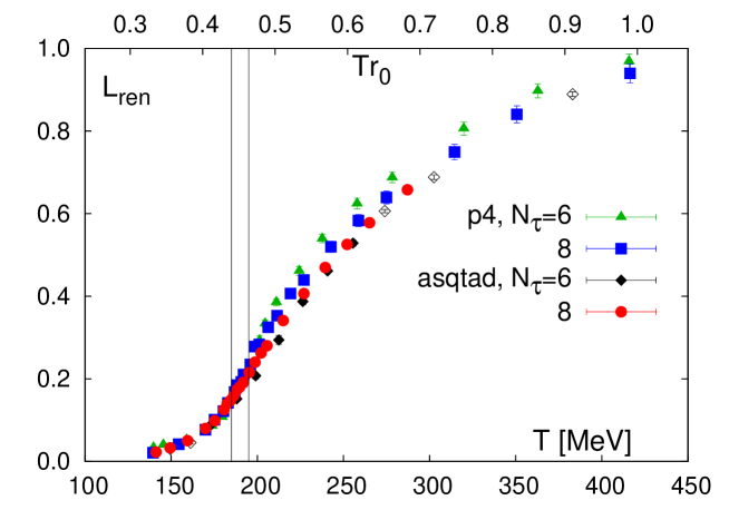
Figure 13: (color online) The renormalized Polyakov loop obtained with the asqtad and p4 actions from simulations on lattices with temporal extent $N_{\tau}=6$ and $8$. Open symbols for the $N_{\tau}=6$, asqtad data set denote data obtained with the R algorithm. All other data have been obtained with an RHMC algorithm.

V Conclusions

We have presented new results on the equation of state of QCD with a strange quark mass chosen close to its physical value and two degenerate light quarks with one tenth of the strange quark mass. A comparison of calculations performed with the p4 and asqtad staggered fermion discretization schemes shows that both actions lead to a consistent picture for the temperature dependence of bulk thermodynamic observables as well as other observables that characterize deconfining and chiral symmetry restoring aspects of QCD thermodynamics. The calculations performed on lattices with temporal extent $N_{\tau}=8$ suggest that the deconfinement of light partonic degrees of freedom, which is reflected in the rapid change of the energy density as well as the light quark number susceptibility, goes along with a sudden drop in the chiral condensates, indicating the melting of the chiral condensate. These findings confirm earlier results obtained within these two discretization schemes.

A comparison of results obtained with the asqtad and p4 actions for two different values of the cutoff, $aT=1/6$ and $1/8$, suggests that cutoff effects in both discretization schemes are at most a few percent for temperatures larger than $300$ MeV. In the vicinity of the peak in the trace anomaly, cutoff effects are still about 15% in calculations with the p4 action and at most half that size for the asqtad action. Also, at low temperatures both actions give consistent results. Here, however, further studies with lighter quarks on finer lattices are needed to get better control over cutoff effects that distorted the hadron spectrum and might influence the thermodynamics in the chiral symmetry broken phase.

We find that different observables give a consistent characterization of the transition region, $180$ MeV $\raise 1.29167pt\hbox{$<$\kern-7.5pt\raise-4.73611pt\hbox{$\sim$}}T\raise 1.29167pt\hbox{$<$\kern-7.5pt\raise-4.73611pt\hbox{$\sim$}}$ $200$ MeV. A comparison of results obtained on lattices with temporal extent $N_{\tau}=6$ and $8$ shows that with decreasing lattice spacing the transition region shifts by about 5–7 MeV towards smaller values of the temperature. Assuming that cutoff effect are indeed ${\cal O}(a^{2})$ for our current simulation parameters, one may expect a shift of similar magnitude when extrapolating to the continuum limit. Preliminary studies of the quark mass dependence of the transition region Soeldner suggest that a shift of similar magnitude is to be expected when the ratio of light to strange quark masses is further reduced to its physical value, $m_{s}/m_{q}\simeq 25$. A more detailed analysis of the transition region, its quark mass and cutoff dependence, will be discussed in a forthcoming publication hotTc .

Appendix A EoS with improved staggered fermion actions

In this appendix we review and collect details of the p4 Heller and asqtad Orginos staggered improved actions to present a unified framework for the description of thermodynamic calculations presented in this paper.

A.1 The asqtad and p4 actions

The QCD partition function on a lattice of size $N_{\sigma}^{3}N_{\tau}$ is written as

$$Z_{LCP}(\beta,N_{\sigma},N_{\tau})=\int\prod_{x,\mu}{\rm d}U_{x,\mu}{\rm e}^{-S(U)}\;\;,$$ (17)

where $U_{x,\mu}\in SU(3)$ denotes the gauge link variables, and

$$S(U)=\beta S_{G}(U,u_{0}(\beta))-S_{F}(U,u_{0}(\beta))$$ (18)

is the Euclidean action. We define the tadpole coefficient $u_{0}$ as $u_{0}=\langle P\rangle_{0}^{1/4}$ where $P$ is the $1\times 1$ Wilson loop called the plaquette and defined below in Eq. (22). After integration over the fermion fields the QCD action is written as the sum of a purely gluonic contribution, $S_{G}$, and the fermionic contribution, $S_{F}$, involving only the gauge fields

$$S_{F}(U,u_{0}(\beta)) = \frac{1}{2}{\rm Tr}\ln D(u_{0}(\beta),\hat{m}_{l}(\beta))+\frac{1}{4}{\rm Tr}\ln D(u_{0}(\beta),\hat{m}_{s}(\beta))\;\;.$$ (19)

Here the factors $1/2$ and $1/4$ arise from taking the square root and the fourth root of the staggered fermion determinant to represent the contribution of 2 degenerate light flavors and the single strange flavor to the QCD partition function root . We show the explicit lattice-coordinate components of the Dirac operator (fermion matrix) and write it in terms of its diagonal and off-diagonal contributions,

$$D_{xy}(u_{0}(\beta),\hat{m}_{i}(\beta))=\hat{m}_{i}(\beta)\delta_{xy}+M_{xy}(u_{0}(\beta))\;.$$ (20)

We also introduce the shorthand notation $D_{i}=\hat{m}_{i}+M=D(u_{0}(\beta),\hat{m}_{i}(\beta))$.

In Eqs. (18) to (20) we made explicit the dependence on $\beta$, $i.e.$ in addition to the explicit multiplicative $\beta$-dependence in front of $S_{G}$ the actions also depend on $\beta$ through the tadpole factor $u_{0}$.

The general form of the gluonic part of the action as it is used in the asqtad and p4 actions is given in terms of a 4-link plaquette term (pl), a planar 6-link rectangle (rt) and a twisted 6-link loop (pg),

$$S_{G}=\sum_{x,\mu<\nu}\left(\beta_{\rm pl}(1-P_{\mu\nu})+\beta_{\rm rt}(1-R_{\mu\nu})\right)+\beta_{\rm pg}\sum_{x,\mu<\nu<\sigma}(1-C_{\mu\nu\sigma})\;,$$ (21)

with $\mu,\;\nu,\;\sigma\in 1,\;2,\;3,\;4$ and $P_{\mu\nu}$, $R_{\mu\nu}$ and $C_{\mu\nu\sigma}$ denote the normalized trace of products of gauge field variables $U_{x,\mu}$:

$$P_{\mu\nu} = \frac{1}{3}{\rm Re\;Tr}\;U_{x,\mu}U_{x+\hat{\mu},\nu}U^{\dagger}_{x+\hat{\nu},\mu}U^{\dagger}_{x,\nu}$$

$$R_{\mu\nu} = \frac{1}{6}{\rm Re\;Tr}\left(U_{x,\mu}U_{x+\hat{\mu},\mu}U_{x+2\hat{\mu},\nu}U^{\dagger}_{x+\hat{\mu}+\hat{\nu},\mu}U^{\dagger}_{x+\hat{\nu},\mu}U^{\dagger}_{x,\nu}+(\mu\leftrightarrow\nu)\right)$$

$$C_{\mu\nu\sigma} = \frac{1}{12}{\rm Re\;Tr}\left(U_{x,\mu}U_{x+\hat{\mu},\nu}U_{x+\hat{\mu}+\hat{\nu},\sigma}U^{\dagger}_{x+\hat{\nu}+\hat{\sigma},\mu}U^{\dagger}_{x+\hat{\sigma},\nu}U^{\dagger}_{x,\sigma}\right.$$ (22)

$$\hskip 44.10185pt\left.+(\mu\leftrightarrow\nu)+(\nu\leftrightarrow\sigma)+(\mu\leftrightarrow\nu,\;\mu\leftrightarrow-\mu)\right)\;,$$

where $\hat{\mu}$ is the unit vector in $\mu$-direction. The p4 action only contains the first two terms, while the asqtad action contains all three terms with $\beta$-dependent couplings. The set of couplings for both actions is given in Table 3.

	$\beta_{pl}$	$\beta_{\rm rt}$	$\beta_{\rm pg}$	$\beta^{\prime}_{\rm rt}$	$\beta^{\prime}_{\rm pg}$	$c_{1}$	$c_{3}$	$c_{12}$
p4	$\displaystyle{\frac{5}{3}}$	$\displaystyle{-\frac{1}{6}}$	0	0	0	$\displaystyle{\frac{3}{8}}$	0	$\displaystyle{\frac{1}{96}}$
asqtad	1	$\displaystyle{-\frac{1}{10u_{0}^{2}}(1+0.4805\alpha_{s})}$	$\displaystyle{-0.1330\frac{1}{u_{0}^{2}}\alpha_{s}}$	$\displaystyle{\frac{1}{5u_{0}^{3}}\left(1.3132+0.4805\alpha_{s}\right)}$	$\displaystyle{\frac{1}{u_{0}^{3}}\left(0.1734+0.2660\alpha_{s}\right)}$	$\displaystyle\frac{1}{2}$	$\displaystyle-\frac{1}{48u_{0}^{2}}$	$\displaystyle 0$

Table 3: Couplings $\beta_{x}$, $x=$ pl, rt, pg defining the pure gauge part of the p4 and asqtad actions, respectively. Here $u_{0}$ is the tadpole coefficient and $\alpha_{s}=-4\ln(u_{0})/3.0684$. Also given are the derivatives $\beta^{\prime}_{x}(u_{0})={\rm d}\beta_{x}/{\rm d}u_{0}$ and the values of the coefficients $c_{i}$ which appear in the fermion part of the action.

We note here a difference in convention that exists between the asqtad and p4 actions. In the asqtad action, the full constant factor in front of the plaquette term is defined to be $\beta$. In the continuum limit, its relation to the gauge coupling $g^{2}$ is $\beta=10/g^{2}$. In the p4 action, the convention of the standard Wilson plaquette action has been kept, $\beta=6/g^{2}$. For this reason the plaquette term contains an extra factor $\beta_{\rm pl}=5/3$. Also note that the pure gauge part of the asqtad action reduces to that of the p4 action for $u_{0}=1$.

The fermionic part of the action has been improved by introducing higher order difference schemes (one-link and three-link terms) to discretize the derivative in the kinetic part of the action Nai89 ,

$$D[U]_{ij} = m~{}\delta_{ij}+\Big{(}c_{1}~{}{A[U]_{ij}}+c_{3}~{}{B_{1}[U]_{ij}}+c_{12}~{}{B_{2}[U]_{ij}}\Big{)}$$ (23)

$${A[U]_{ij}} = \sum_{\mu}\eta_{\mu}(i)\Big{(}U_{i,\mu}^{\rm fat}\delta_{i\;j-\hat{\mu}}-U_{i-\hat{\mu},\mu}^{{\rm fat}\dagger}\delta_{i\;j+\hat{\mu}}\Big{)}$$

$${B_{1}[U]_{ij}} = \sum_{\mu}\eta_{\mu}(i)\Big{(}U_{i,\mu}U_{i+\hat{\mu},\mu}U_{i+2\hat{\mu},\mu}\delta_{i\;j-3\hat{\mu}}-U_{i-\hat{\mu},\mu}^{\dagger}U_{i-2\hat{\mu},\mu}^{\dagger}U_{i-3\hat{\mu},\mu}^{\dagger}\delta_{i\;j+3\hat{\mu}}\Big{)}$$

$$B_{2}[U]_{ij} = \sum_{\mu}\eta_{\mu}(i)\sum_{\nu\neq\mu}\bigg{[}\Big{(}U_{i,\mu}U_{i+\hat{\mu},\nu}U_{i+\hat{\mu}+\hat{\nu},\nu}\delta_{i\;j-\hat{\mu}-2\hat{\nu}}-U_{i-\hat{\nu},\nu}^{\dagger}U_{i-2\hat{\nu},\nu}^{\dagger}U_{i-\hat{\mu}-2\hat{\nu},\mu}^{\dagger}\delta_{i\;j+\hat{\mu}+2\hat{\nu}}\Big{)}$$

$$~{}~{}~{}+\Big{(}U_{i,\nu}U_{i+\hat{\nu},\nu}U_{i+2\hat{\nu},\mu}\delta_{i\;j-\hat{\mu}-2\hat{\nu}}-U_{i-\hat{\mu},\mu}^{\dagger}U_{i-\hat{\mu}-\hat{\nu},\nu}^{\dagger}U_{i-\hat{\mu}-2\hat{\nu},\nu}^{\dagger}\delta_{i\;j+\hat{\mu}+2\hat{\nu}}\Big{)}$$

$$~{}~{}~{}+\Big{(}U_{i-\hat{\nu},\nu}^{\dagger}U_{i-2\hat{\nu},\nu}^{\dagger}U_{i-2\hat{\nu},\mu}\delta_{i\;j-\hat{\mu}+2\hat{\nu}}-U_{i-\hat{\mu},\mu}^{\dagger}U_{i-\hat{\mu},\nu}U_{i-\hat{\mu}+\hat{\nu},\nu}\delta_{i\;j+\hat{\mu}-2\hat{\nu}}\Big{)}$$

$$~{}~{}~{}+\Big{(}U_{i,\mu}U_{i+\hat{\mu}-\hat{\nu},\nu}^{\dagger}U_{i+\hat{\mu}-2\hat{\nu},\mu}^{\dagger}\delta_{i\;j-\hat{\mu}+2\hat{\nu}}-U_{i,\nu}U_{i+\hat{\nu},\nu}U_{i-\hat{\mu}+2\hat{\nu},\mu}^{\dagger}\delta_{i\;j+\hat{\mu}-2\hat{\nu}}\Big{)}\bigg{]}\;.$$

Here $\eta_{\mu}(i)$ denotes the staggered phase factor. The coefficients $c_{1}$, $c_{3}$ and $c_{12}$ for p4 and asqtad actions are also given in Table 3. The overall normalization is such that in the limit $\beta\rightarrow\infty$ we recover the naive continuum action for Dirac fermions. In both actions, so-called fat links ($U^{\rm fat}$) have been introduced in the 1-link terms; i.e., in addition to the straight 1-link parallel transporter $U_{x,\mu}$ that connects adjacent sites $(x,x+\hat{\mu})$, additional longer paths have been added. In the case of the p4 action, this is a simple three-link path, called the staple, going around an elementary plaquette. The coefficients of the 1-link term and the staple are $\beta$-independent and equal to $1/(1+6\omega)$ and $\omega/(1+6\omega)$, respectively. We used $\omega=0.2$ Peikert . The asqtad fat-link contains additional non-planar 5-link and 7-link paths to remove completely the effect of flavor symmetry breaking to order $(g^{2}a^{2})$ Orginos as well as a planar 5-link path, the so-called Lepage term. The coefficient of the one link term in this case is equal to $5/8$. The coefficients of the 3-, 5- and 7-link paths are equal to $1/(2u_{0}^{2})(1/8),~{}1/(8u_{0}^{4})(1/8)$ and $1/(48u_{0}^{6})(1/8)$, respectively. Furthermore, the coefficient of the Lepage term is $-1/(16u_{0}^{4})$.

Finally, we point out that the conventions for the asqtad fermion matrix given in Orginos1 differ from those introduced in Eqs. (20) and (23) by an overall factor two. Thus, all couplings given in Orginos need to be divided by a factor two to match the expressions given here.

A.2 $\beta$-functions

In this work, we consider the thermodynamics of ($2+1$)-flavor QCD along a line of constant physics (LCP). The LCP is fixed by choosing two degenerate light ($\hat{m}_{l}$) and a heavier (strange) quark mass ($\hat{m}_{s}$) as functions of the gauge coupling $\beta$, i.e. $\hat{m}_{l,s}\equiv\hat{m}_{l,s}(\beta)$, such that physical observables, e.g. a set of hadron masses, calculated at $T=0$ at the same value of the cutoff as used at finite temperature, stay constant. In calculations with the asqtad as well with the p4 action, it turns out that a LCP is well characterized by specifying $\hat{m}_{l}(\beta)$ and keeping the ratio $\hat{m}_{l}/\hat{m}_{s}$ fixed. Explicit parametrizations for $\hat{m}_{l}(\beta)$ have been given for the asqtad milc_eos and p4 rbcBIeos actions for $\hat{m}_{l}/\hat{m}_{s}=0.1$ in the parameter range relevant for the thermodynamic calculations discussed here.

The basic observable we need to calculate is the trace anomaly, $\epsilon-3p$, introduced in Eq. (2). To do so, we need to relate temperature changes to changes of the gauge coupling. These are controlled by the $\beta$-function,

$$R_{\beta}=T\frac{{\rm d}\beta}{{\rm d}T}=-a\frac{{\rm d}\beta}{{\rm d}a}\;.$$ (24)

The $\beta$-function can be determined by analyzing the $\beta$-dependence of a physical observable expressed in lattice units. We use here distance scales $r_{n}$ extracted from the heavy quark potential as introduced in Eq. (1). Explicit parametrizations for $\hat{r}_{0}(\beta)$ (p4-action) and $\hat{r}_{1}(\beta)$ (asqtad action) have been given in rbcBIeos and milc_eos , respectively. Using the explicit parametrizations for $\hat{r}_{n}$ and $\hat{m}_{l}$ we can determine the $\beta$-function $R_{\beta}$ and the mass renormalization function $R_{m}$,

$$R_{\beta}(\beta)=\hat{r}_{n}\left(\frac{{\rm d}\hat{r}_{n}}{{\rm d}\beta}\right)^{-1}\;,\;R_{m}(\beta)=\frac{1}{\hat{m}_{l}(\beta)}\frac{{\rm d}\hat{m}_{l}(\beta)}{{\rm d}\beta}\;.$$ (25)

In the case of the asqtad action one more function plays a central role in the derivation of general expressions for thermodynamic quantities. This is the tadpole coefficient $u_{0}(\beta)$ which enters the definition of the asqtad action. It is given in terms of the plaquette expectation value at zero temperature, $u_{0}=\langle P\rangle_{0}^{1/4}$, where $P$ denotes the product of gauge field variables defined on an elementary plaquette of the 4-dimensional lattice. It is introduced in Eq. (22). As discussed previously, the p4 action contains only tree-level improved terms without tadpole improvement. In order to keep the following formulas valid for both actions, we insert $u_{0}\equiv 1$ as a trivial constant in the p4 action.

Since $u_{0}$ depends on $\beta$ for the asqtad action, we also need it’s derivative with respect to $\beta$,

$$R_{u}(\beta)=\beta\frac{{\rm d}u_{0}(\beta)}{{\rm d}\beta}\;.$$ (26)

This is obtained from the polynomial parametrization used for interpolating the value of the tadpole factor in the asqtad action,

$$u_{0}(\beta)=a_{0}+a_{1}b+a_{2}b^{2}+a_{3}b^{3}+a_{4}b^{4}+a_{5}b^{5}+a_{6}b^{6}\;,$$ (27)

with $b=\beta-6.60$, $a_{0}=0.86158$, $a_{1}=0.0426043$, $a_{2}=-0.0254633$, $a_{3}=0.0261288$, $a_{4}=-0.0116944$, $a_{5}=-0.0417343$, and $a_{6}=0.0436528$. This parametrization is suitable for the $\beta$-range covered by the calculations presented in this work. In the weak coupling limit $R_{u}\sim\beta^{-1}$.

A.3 Thermodynamics

Having established the notation, we now present expressions for basic thermodynamic quantities calculated with the asqtad and p4 actions.

The light and strange quark condensates calculated at finite ($x=\tau$) and zero ($x=0$) temperature are

$$\langle\bar{\psi}\psi\rangle_{q,x}\equiv\frac{1}{4}\frac{1}{N_{\sigma}^{3}N_{x}}\left\langle{\rm Tr}D_{q}^{-1}\right\rangle_{x}\;\;,\;\;q=l,~{}s\;\;,\;\;x=0,~{}\tau\;\;.$$ (28)

Here $N_{x}$, with $x=0,\;\tau$ denotes the temporal extent of zero and finite temperature lattices, and $N_{\sigma}$ is the size in the spatial directions. The action densities are then given by

$$s\equiv\frac{1}{N_{\sigma}^{3}N_{x}}S\;\;{\rm for}\;\;x=0,~{}\tau$$ (29)

and similarly for $S_{G}$ and $S_{F}$. We introduce a short-hand notation for differences of expectation values of intensive observables calculated at finite and zero temperature as

$$\Delta\left\langle X\right\rangle=\left\langle X\right\rangle_{0}-\left\langle X\right\rangle_{\tau}\;.$$ (30)

The trace anomaly is then given by

$$\frac{\epsilon-3p}{T^{4}}=\frac{\Theta^{\mu\mu}(T)}{T^{4}} = R_{\beta}(\beta)N_{\tau}^{4}\Delta\left\langle s\right\rangle\;,$$ (31)

and Eq. (31) can be rewritten as

$$\frac{\Theta^{\mu\mu}(T)}{T^{4}} = \frac{\Theta^{\mu\mu}_{G}(T)}{T^{4}}+\frac{\Theta^{\mu\mu}_{F}(T)}{T^{4}}\;\;,$$ (32)

with $\Theta^{\mu\mu}_{F}(T)/T^{4}$ denoting the contribution from the renormalization group invariant contribution of light and strange quark condensates,

$$\frac{\Theta^{\mu\mu}_{F}(T)}{T^{4}} = -R_{\beta}R_{m}N_{\tau}^{4}\left(2\hat{m}_{l}\Delta\left\langle\bar{\psi}\psi\right\rangle_{l}+\hat{m}_{s}\Delta\left\langle\bar{\psi}\psi\right\rangle_{s}\right)\;,$$ (33)

and ${\Theta^{\mu\mu}_{G}(T)/T^{4}}$ including all the remaining terms that would survive the chiral limit ($m_{l,s}\rightarrow 0$),

$$\frac{\Theta^{\mu\mu}_{G}(T)}{T^{4}} = R_{\beta}N_{\tau}^{4}\left(\Delta\left\langle s_{G}\right\rangle-R_{u}\left(6\beta^{\prime}_{\rm rt}\Delta\left\langle R\right\rangle+4\beta^{\prime}_{\rm pg}\Delta\left\langle C\right\rangle+\frac{1}{4\beta}\Delta\left\langle{\rm Tr}\left(\left(2D_{l}^{-1}+D_{s}^{-1}\right)\frac{dM}{du_{0}}\right)\right\rangle\right)\right)\;.$$ (34)

Here $\left\langle s_{G}\right\rangle$ denotes the contribution of the gluonic action density and $\left\langle R\right\rangle$ and $\left\langle C\right\rangle$ denote the expectation values of 6-link Wilson loops introduced in Eq. (22). The functions $\beta^{\prime}_{\rm rt}$ and $\beta^{\prime}_{\rm pg}$ are given in Table 3. We have explicitly separated contributions proportional to the derivative of the tadpole coefficient, $R_{u}$. As $R_{u}\equiv 0$ for the tree level improved p4 action, these terms contribute only in calculations with the asqtad action, where they help to reduce the cutoff dependence of thermodynamic observables at nonzero lattice spacing.

In Appendix D we also use the obvious short hand notation for light and strange fermion contributions, $\displaystyle{\Theta^{\mu\mu}_{F}(T)/T^{4}=\Theta^{\mu\mu}_{F,l}(T)/T^{4}+\Theta^{\mu\mu}_{F,s}(T)/T^{4}}$.

Appendix B Polyakov loop renormalization for the asqtad action

To renormalize the Polyakov loop we use an approach similar to the one of Ref. rbcBIeos : we renormalize the static quark potential and extract the self-energy of a static quark. At a given lattice spacing the latter is simply a constant shift of the potential which we denote $C(\beta)$. As a matching condition we have chosen the same one as for the p4 action: the renormalized potential is set equal to the string potential $V_{string}(r)=-\pi/12r+\sigma r$ at distance $r=1.5r_{0}$. We first fit the static potential measured from the ratios of the correlators of Wilson lines in the Coulomb gauge to the ansatz:

$$V(r,\beta)=V_{0}-\frac{1.65-\sigma r_{0}^{2}}{r}+\sigma r$$ (35)

with $V_{0}$, $\sigma$, $r_{0}$ being the fit parameters, and then apply the conditions:

$$V(r,\beta) = V_{ren}(r,\beta)+C(\beta),$$ (36)

$$V_{ren}(r=1.5r_{0},\beta) = V_{string}(r=1.5r_{0}).$$ (37)

This gives

$$C(\beta)=V_{0}+\frac{1}{1.5r_{0}}\left(\frac{\pi}{12}-1.65+\sigma r_{0}^{2}\right).$$ (38)

The results for $C(\beta)$ are collected in Table 4. The renormalization of the Polyakov loop amounts to removing the self-energy contribution

$$L_{ren}(\beta)=L(\beta)e^{(C(\beta)/a)/(2T)}=L(\beta)\left(Z(\beta)\right)^{N_{\tau}},$$ (39)

where we defined

$$Z(\beta)=e^{C(\beta)/2}$$ (40)

for convenience. In Fig. 14, $Z(\beta)$ data is shown together with the fit to a quadratic polynomial. The error band is estimated with a bootstrap analysis.

$\beta$	$C(\beta)$
6.100	0.746(69)
6.300	0.777(23)
6.458	0.8534(89)
6.550	0.8425(47)
6.650	0.8584(78)
6.760	0.8545(35)
6.850	0.863(15)
7.080	0.8335(22)

Table 4: Twice the self energy of a static quark $C(\beta)$ in lattice units along the line of constant physics $m_{l}=0.1m_{s}$.

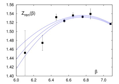
Figure 14: (color online) The renormalization constant $Z(\beta)$. The error band is determined with bootstrap analysis.

Appendix C Parametrizing the Equation of State for Hydrodynamics

Here we present a simple functional form for generating the equation of state that can be readily applied to most hydrodynamic models of heavy ion collisions. The equation of state is an essential input for solving the hydrodynamic equations of motion, but as explained in Section II.2, some form of interpolation of the interaction measure is required to generate the equation of state from the lattice data. However, small fluctuations in the equation of state can be magnified through the time evolution in the hydrodynamic models and can lead to anomalous effects in the final state. Furthermore, it is preferable for the equation of state to transition smoothly to the EoS of the hadronic resonance gas that is imposed when the models freeze-out to produce final state hadrons. Most hydrodynamic models use a simplified version of the equation of state that incorporates a hadronic resonance gas EoS below the transition. Near and above the transition some models approximates the crossover EoS calculated on the lattice Huovinen:2005gy ; Luzum:2008cw ; Pratt:2008qv , but it is more common for hydro models to rely on a bag model equation of state with a first order phase transition Kolb:2002ve ; Hirano:2005wx ; Nonaka:2007bj .

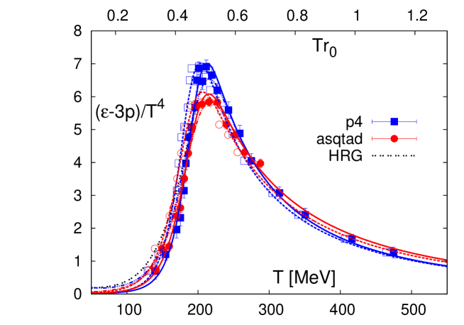
Figure 15: (color online) Fits to the trace anomaly using Eq. (41) for p4 and asqtad $N_{\tau}=8$ lattice data (solid lines), to lattice data merged with the hadron resonance gas calculation ($m_{res}<2.5$ GeV) over the region $100<T<130$ MeV (double-dot dashed), and to the lattice data shifted to lower temperature by 10 MeV (dashed).

To remedy this gap between theory and phenomenology we fit the lattice calculation of the trace anomaly for both p4 and asqtad actions to the simple functional form given by Eq. (41).

$$\frac{\epsilon-3p}{T^{4}}=\left(1-\frac{1}{[1+e^{(T-c_{1})/c_{2})}]^{2}}\right)\left(\frac{d_{2}}{T^{2}}+\frac{d_{4}}{T^{4}}\right)$$ (41)

This form uses a modified hyperbolic tangent to describe the transition region and retains the high temperature region ansatz of Eq. (5). For the p4 action, the high temperature parameters are set to the values obtained in Section II.2.2 for the range $T>0.25$ GeV. We repeat this procedure for the asqtad action, but with the fourth order term $d_{4}$ set to zero due to the lack of high temperature measurements to constrain it. The high temperature parameters are then fixed as the full function of Eq. (41) is fit to the lattice data or to some combination of lattice data and hadronic resonance gas. In this way we prevent any deficiencies in the description of the transition and peak region from biasing the high temperature behavior, although variations at low temperature will produce offsets in the pressure and energy density at high temperature. To match to the HRG EoS we adopt a procedure that is similar to systematic error analysis of Section III in which the HRG was used establish the starting value for the integration of the pressure at 100 MeV. However, to achieve a gradual transition we incorporate the HRG calculation for $m_{res}<2.5$ GeV over a range of temperatures $100<T<130$ MeV. HRG values for the trace anomaly are sampled every 5 MeV and assigned an error of 0.1 to produce weights that are comparable to the low temperature lattice data.

Fig. 15 shows the result of fitting Eq. (41) to the p4 and asqtad $N_{\tau}$ trace anomaly (solid lines). The trace anomaly for the resonance gas is also plotted (double dotted), along with fits to the both p4 and asqtad data that are combined with the HRG for $100<T<130$ MeV. As an additional test of this parametrization, we also fit to the lattice data shifted to lower temperature by 10 MeV (open symbols). Based on the comparison to $N_{\tau}=6$ shown in Fig. 3, we expect that the continuum extrapolation will lead to shifts that are no greater than this amount. These fits follow the same prescription: the high temperature component is fit first and these parameters are fixed for the full minimization (dashed lines).

Data	$d_{2}$ [GeV]2	$d_{4}$ [GeV]4	$c_{1}$ [GeV]	$c_{2}$ [GeV]	$\chi^{2}$/dof
p4	0.24(2)	0.0054(17)	0.2038(6)	0.0136(4)	26.7/19
p4-10 MeV	0.241(6)	0.0035(9)	0.1938(6)	0.01361(4)	26.7/19
HRG+p4	0.24(2)	0.0054(17)	0.2073(6)	0.0172(3)	–
asq	0.312(5)	0.00	0.2024(6)	0.0162(4)	34.4/14
asq-10 MeV	0.293(6)	0.00	0.1943(6)	0.01670(4)	42.8/14
HRG+asqtad	0.312(5)	0.00	0.2048(6)	0.0188(4)	–

Table 5: Parameter values for fits of Eq. (41) to trace anomaly data for p4 and asqtad, data combined with HRG calculations, and data shifted by 10 MeV.

The parameters for all fits are listed in Tab. 5. As is readily seen in Fig. 15 and the $\chi^{2}/ndf$ reported for the lattice fits in Tab. 5, this functional form provides only an approximation to the full lattice calculation, but one that will be shown to be within the systematic errors for the equation of state. As statistical and systematic errors are reduced in future calculations, the parametrization of Eq. (41) is easily modified to include additional terms, including the high temperature perturbative terms. The shift by 10 MeV has the predictable effect of lowering the $c_{1}$ parameter by a similar amount. Including the HRG points affects mainly the exponential slope term $c_{2}$ leading to a slight reduction of the peak.

The energy density and pressure are calculated by numerically integrating the trace anomaly fits according to Eq. (3). For these parametrizations the integration is started at 50 MeV. Because these parametrizations of the trace anomaly have their minima in this region, the pressure and energy density are not sensitive to the exact location of the starting temperature. We note, however, that Eq. (15) rises rapidly as the temperature is further reduced, and is not suitable for extrapolating to temperatures less than 50 MeV, well below the freeze-out temperature for all hydrodynamic calculations for relativistic heavy ion collisions.

Figure 16 shows the energy density and pressure curves for all fits compared to the systematic error calculations that were described in Section III. These parametrized curves do not differ appreciably from the p4 and asqtad results shown in Fig. 7, except that the asqtad equation of state has been extrapolated beyond the highest temperature data point at $\sim$400 MeV. Fits to the HRG merged to asqtad data lead to small increases in the pressure but they are within the systematic errors associated with the interpolation, shown as shaded boxes. They shaded boxes were drawn as narrow error bars in Fig. 7 that were centered on the p4 interpolation pressure curves. The HRG+p4 merged and 10 MeV shifted data fits lie slightly above this systematic, but fall below the systematic error associated with using the HRG value for the pressure to begin the integration at $T=100$ MeV, as plotted here as shaded band in the energy density. This error bar was shown as a shaded box at high temperature in Fig. 7. The agreement between the p4 and asqtad results at the highest temperature provides some confidence in using the high temperature parametrization to extrapolate the asqtad result up to 550 MeV. At this temperature, all parametrizations are below the Stefan-Boltzmann limit.

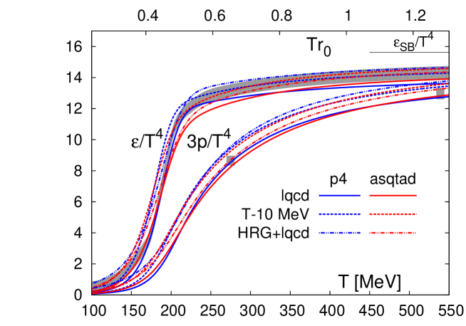
Figure 16: (color online) Energy density and 3 times the pressure calculated from new fitting Eq. (41) to the trace anomaly. Fits to p4 and asqtad lattice data are solid lines, fits to lattice data shifted by negative 10 MeV are dashed lines, and combined fits to HRG and lattice data are double-dot dashed. The systematic error band associated with beginning the pressure integration at $T=100$ MeV and plotted as a black shaded box in Fig. 7 is plotted as a grey band, with lower bound defined by the pressure integration derived from the p4 interpolation. The systematic errors associated the interpolation are plotted here as grey boxes. These were shown as narrow error bars in Fig. 7.

Figure 17: (color online) Square of the velocity of sound, $c_{s}^{2}$, for the Eq. (41) parametrization of the trace anomaly for fits to the lattice data (solid) lattice data shifted by 10 MeV (dashed), and combined HRG and lattice calculations (double-dot dashed). The lattice curves are compared to two typically EoS inputs currently used in hydrodynamic codes: the qcdEOS used in vh2 (dotted), and a HRG calculation with a first order transition at 180 MeV (double-dotted).

The square of the velocity of sound is shown in Fig. 17, as given by Eq. (9). Differences between the fits are mainly evident at lower temperatures. The parametrizations for p4 and asqtad uniformly approach but do not attain the ideal gas limit shown for the HRG calculations with first order phase transition. The latter is typical for many of the hydrodynamic calculations that are represented in the literature. The EoS employed by the publicly available Viscous Hydro 2D+1 code (VH2) Luzum:2008cw comes close to the set of lattice curves but falls somewhat below these new lattice results at higher temperatures.

Appendix D Summary of expectation values needed to calculate the trace anomaly

The various expectation values needed to evaluate the trace anomaly are summarized in Tables 6 and 7 for the p4 action and in Tables 8 to 13 for the asqtad action.

$\beta$	$m_{l}$	$N_{\sigma}^{3}\times N_{\tau}$	$\tau_{MD}$	traj	$\langle s_{G}\rangle_{0}$	$\langle\bar{\psi}\psi\rangle_{l,0}$	$\langle\bar{\psi}\psi\rangle_{s,0}$
3.4300	0.00370	$32^{3}\times 32$	0.5	3570	4.111679(148)	0.075873(102)	0.143475(74)
3.4600	0.00313	$32^{3}\times 32$	1.0	2060	4.044602(82)	0.057641(85)	0.117406(61)
3.4900	0.00290	$32^{3}\times 32$	0.5	2330	3.984160(149)	0.044554(87)	0.100634(57)
3.5000	0.00253	$32^{3}\times 32$	0.5	2150	3.964162(117)	0.039426(93)	0.089291(68)
3.5100	0.00259	$32^{3}\times 32$	0.5	1790	3.946336(118)	0.036767(61)	0.087441(51)
3.5150	0.00240	$32^{3}\times 32$	1.0	2100	3.936885(100)	0.034644(64)	0.081973(45)
3.5225	0.00240	$32^{3}\times 32$	1.0	2210	3.923687(111)	0.032628(87)	0.079799(56)
3.5300	0.00240	$32^{3}\times 32$	0.5	2870	3.910643(78)	0.030849(38)	0.077800(25)
3.5400	0.00240	$32^{3}\times 32$	0.5	3750	3.893451(86)	0.028546(63)	0.075221(48)
3.5450	0.00215	$32^{3}\times 32$	0.5	2270	3.884507(105)	0.026400(77)	0.068601(61)
3.5500	0.00211	$32^{3}\times 32$	0.5	2650	3.876406(101)	0.025483(45)	0.066852(31)
3.5600	0.00205	$32^{3}\times 32$	1.0	2090	3.859529(88)	0.023064(85)	0.063168(53)
3.5700	0.00200	$32^{3}\times 32$	0.5	1880	3.843775(75)	0.021405(57)	0.060291(36)
3.5850	0.00192	$32^{3}\times 32$	0.5	2310	3.820193(102)	0.019054(55)	0.056042(43)
3.6000	0.00192	$32^{3}\times 32$	0.5	3020	3.797184(65)	0.017178(38)	0.053636(28)
3.6300	0.00170	$24^{3}\times 32$	0.5	3232	3.752910(95)	0.013176(93)	0.045175(64)
3.6600	0.00170	$32^{3}\times 32$	0.5	2850	3.710875(72)	0.011655(39)	0.042370(27)
3.6900	0.00150	$24^{3}\times 32$	0.5	2284	3.669910(81)	0.008740(85)	0.035734(45)
3.7600	0.00139	$32^{3}\times 32$	0.5	3250	3.580229(48)	0.006227(29)	0.029547(12)
3.8200	0.00125	$32^{3}\times 32$	0.5	2430	3.508141(72)	0.004507(69)	0.024679(37)
3.9200	0.00110	$32^{3}\times 32$	0.5	4670	3.396463(44)	0.002970(41)	0.019633(9)
4.0000	0.00092	$32^{3}\times 32$	0.5	5430	3.313344(46)	0.001788(28)	0.015390(21)
4.0800	0.00081	$32^{3}\times 32$	0.5	5590	3.234959(32)	0.001552(54)	0.012778(19)

Table 6: Parameters for simulations performed with the p4 action at zero temperature and the expectation values of the gauge action and light and heavy chiral condensates. Here we used also the zero temperature results from the study of the equation of state by RBC-Bielefeld collaboration at $\beta=3.63$, 3.69, 3.82, and 3.92 rbcBIeos .

$T$[MeV]	$\beta$	$m_{l}$	$\tau_{MD}$	traj	$\langle s_{G}\rangle_{\tau}$	$\langle\bar{\psi}\psi\rangle_{l,\tau}$	$\langle\bar{\psi}\psi\rangle_{s,\tau}$	$\Theta_{G}^{\mu\mu}/T^{4}$	$\Theta_{F,l}^{\mu\mu}/T^{4}$	$\Theta_{F,s}^{\mu\mu}/T^{4}$
139	3.4300	0.00370	0.5	15140	4.111274(146)	0.074251(111)	0.142977(75)	0.48(25)	0.0433(42)	0.133(28)
154	3.4600	0.00313	0.5	11970	4.043850(110)	0.055231(83)	0.116653(58)	0.95(18)	0.0512(32)	0.160(20)
170	3.4900	0.00290	0.5	11800	3.983028(116)	0.040290(103)	0.099071(65)	1.53(27)	0.0758(30)	0.278(17)
175	3.5000	0.00253	1.0	10070	3.962857(99)	0.034018(145)	0.087194(75)	1.81(23)	0.0806(33)	0.312(18)
180	3.5100	0.00259	0.5	12660	3.944532(104)	0.030218(98)	0.084857(59)	2.58(24)	0.0958(21)	0.378(13)
183	3.5150	0.00240	1.0	10110	3.934529(79)	0.026463(138)	0.078531(66)	3.41(20)	0.1085(25)	0.456(12)
187	3.5225	0.00240	0.5	30620	3.920960(122)	0.023138(237)	0.075811(122)	4.02(25)	0.1218(34)	0.512(17)
191	3.5300	0.00240	0.5	43480	3.907753(92)	0.020257(149)	0.073347(81)	4.34(18)	0.1316(19)	0.553(10)
196	3.5400	0.00240	0.5	44880	3.890373(90)	0.016457(137)	0.070059(79)	4.74(21)	0.1439(23)	0.614(13)
199	3.5450	0.00215	0.5	13110	3.880942(187)	0.012615(300)	0.062299(198)	5.55(37)	0.1440(42)	0.658(26)
201	3.5500	0.00211	0.5	30140	3.872654(65)	0.011318(93)	0.060225(62)	5.91(24)	0.1423(22)	0.666(12)
206	3.5600	0.00205	1.0	9500	3.856090(118)	0.008940(96)	0.056184(87)	5.54(30)	0.1328(27)	0.656(17)
211	3.5700	0.00200	0.5	32580	3.840126(77)	0.007533(94)	0.052919(95)	6.01(26)	0.1228(27)	0.653(18)
219	3.5850	0.00192	1.0	4610	3.816785(77)	0.005885(44)	0.048085(83)	5.80(31)	0.1069(23)	0.646(18)
227	3.6000	0.00192	0.5	12750	3.794094(71)	0.005337(16)	0.046010(30)	5.42(27)	0.0925(20)	0.596(14)
243	3.6300	0.00170	0.5	12040	3.750217(76)	0.004032(12)	0.037784(35)	4.99(32)	0.0600(17)	0.485(14)
259	3.6600	0.00170	0.5	10610	3.708640(95)	0.003694(6)	0.035527(27)	4.35(30)	0.0507(10)	0.436(9)
275	3.6900	0.00150	0.5	14630	3.668111(64)	0.003033(3)	0.029784(17)	3.66(25)	0.0318(8)	0.331(6)
315	3.7600	0.00139	0.5	10740	3.578960(68)	0.002536(1)	0.025183(9)	2.81(19)	0.0192(2)	0.228(1)
351	3.8200	0.00125	0.5	15140	3.507192(39)	0.002138(0)	0.021318(6)	2.23(22)	0.0114(5)	0.162(4)
416	3.9200	0.00110	0.5	27180	3.395840(25)	0.001743(0)	0.017408(2)	1.57(17)	0.0054(3)	0.098(3)
475	4.0000	0.00092	0.5	23280	3.312885(38)	0.001390(0)	0.013887(1)	1.21(19)	0.0015(1)	0.057(2)
539	4.0800	0.00081	0.5	24140	3.234697(20)	0.001175(0)	0.011747(0)	1.21(19)	0.0015(1)	0.057(2)

Table 7: Parameters for simulations performed with the p4 action at finite temperatures, the expectation values of the gauge action, light and heavy chiral condensates, as well as the gluonic and fermionic contributions to the trace anomaly obtained from them.

$\beta$	$m_{l}$	traj	$u_{0}$	$\left\langle P\right\rangle$	$\left\langle R\right\rangle$	$\left\langle C\right\rangle$
6.400	0.00909	4830	0.8520	0.526573(7)	0.271218(9)	0.277200(10)
6.430	0.00862	4935	0.8535	0.530550(7)	0.276220(10)	0.282561(10)
6.458	0.00820	6015	0.8549	0.534163(6)	0.280792(8)	0.287447(9)
6.500	0.00765	5390	0.8569	0.539353(5)	0.287379(6)	0.294465(7)
6.550	0.00705	5680	0.8594	0.545370(5)	0.295095(7)	0.302650(7)
6.600	0.00650	5215	0.8616	0.550963(6)	0.302287(8)	0.310253(9)
6.625	0.00624	4890	0.8626	0.553620(7)	0.305709(10)	0.313862(10)
6.650	0.00599	5310	0.8636	0.556230(5)	0.309083(9)	0.317410(9)
6.675	0.00575	5225	0.8647	0.558830(6)	0.312461(9)	0.320960(9)
6.700	0.00552	5055	0.8657	0.561350(4)	0.315727(6)	0.324388(6)
6.730	0.00525	5195	0.8668	0.564267(5)	0.319526(7)	0.328364(8)
6.760	0.00500	4922	0.8678	0.567073(7)	0.323173(9)	0.332197(11)
6.800	0.00471	4755	0.8692	0.570777(4)	0.328002(5)	0.337237(6)
6.850	0.00437	4540	0.8709	0.575240(5)	0.333853(7)	0.343340(8)
6.900	0.00407	4310	0.8726	0.579580(4)	0.339553(7)	0.349283(7)
6.950	0.00380	4285	0.8741	0.583757(4)	0.345060(6)	0.355003(7)
7.000	0.00355	4130	0.8756	0.587820(6)	0.350440(9)	0.360573(10)
7.080	0.00310	3965	0.8779	0.594080(4)	0.358757(6)	0.369187(7)
7.460	0.00180	251	0.8876	0.620817(4)	0.394840(5)	0.406313(5)

Table 8: Simulation parameters at zero temperature for the asqtad action and the expectation values of terms in the gauge action. The column labeled $P$ is the plaquette, $R$, the rectangle, and $C$, the parallelogram. In all cases, the trajectory length is $\tau_{MD}=1$ and the lattice size is $N_{\sigma}\times N_{\tau}=32^{4}$, except for $\beta=7.46$, where it is $64^{3}144$ .

$\beta$	$\langle\bar{\psi}\psi\rangle_{l,0}$	$\langle\bar{\psi}\psi\rangle_{s,0}$	$\left\langle\bar{\psi}\frac{dM}{du_{0}}\psi\right\rangle_{l,0}$	$\left\langle\bar{\psi}\frac{dM}{du_{0}}\psi\right\rangle_{s,0}$
6.400	0.101993(42)	0.222407(30)	$-4.89560(7)$	$-4.82871(7)$
6.430	0.091265(62)	0.207453(43)	$-4.89481(7)$	$-4.83519(9)$
6.458	0.082138(36)	0.194171(26)	$-4.89283(6)$	$-4.83933(6)$
6.500	0.070319(33)	0.176287(24)	$-4.88921(5)$	$-4.84355(5)$
6.550	0.058049(39)	0.156758(28)	$-4.88009(5)$	$-4.84239(5)$
6.600	0.048335(44)	0.139653(30)	$-4.87296(5)$	$-4.84183(5)$
6.625	0.044200(39)	0.131874(31)	$-4.87004(6)$	$-4.84180(6)$
6.650	0.040376(40)	0.124493(32)	$-4.86661(4)$	$-4.84097(4)$
6.675	0.036985(45)	0.117575(29)	$-4.86087(4)$	$-4.83760(5)$
6.700	0.033917(39)	0.111080(25)	$-4.85648(4)$	$-4.83535(4)$
6.730	0.030557(40)	0.103681(30)	$-4.85230(4)$	$-4.83354(4)$
6.760	0.027679(30)	0.096988(21)	$-4.84924(7)$	$-4.83249(6)$
6.800	0.024320(34)	0.089120(23)	$-4.84319(4)$	$-4.82871(4)$
6.850	0.020852(67)	0.080307(42)	$-4.83519(4)$	$-4.82318(5)$
6.900	0.017971(39)	0.072717(28)	$-4.82687(3)$	$-4.81669(4)$
6.950	0.015605(43)	0.066099(27)	$-4.81963(3)$	$-4.81103(4)$
7.000	0.013560(43)	0.060154(26)	$-4.81222(4)$	$-4.80494(3)$
7.080	0.010803(49)	0.050807(28)	$-4.80044(3)$	$-4.79507(3)$
7.460	0.0043819(81)	0.0256237(100)	$-4.74518(2)$	$-4.74365(2)$

Table 9: Continuation of the previous table. Fermion expectation values for the asqtad action contributing to the equation of state. The last two columns give the contributions of asqtad gauge and fermion observables to the interaction measure.

$T$[MeV]	$\beta$	$m_{l}$	traj	$u_{0}$	$\left\langle P\right\rangle$	$\left\langle R\right\rangle$	$\left\langle C\right\rangle$
141	6.458	0.00820	14095	0.8549	0.534193(7)	0.280840(10)	0.287487(11)
149	6.500	0.00765	16943	0.8569	0.539410(7)	0.287467(9)	0.294557(11)
160	6.550	0.00705	14605	0.8594	0.545430(7)	0.295185(10)	0.302728(11)
170	6.600	0.00650	14735	0.8616	0.551060(6)	0.302443(9)	0.310395(10)
175	6.625	0.00624	16610	0.8626	0.553727(5)	0.305883(8)	0.314021(9)
181	6.650	0.00599	16235	0.8636	0.556370(6)	0.309315(9)	0.317627(10)
183	6.658	0.00590	15655	0.8640	0.557250(7)	0.310468(10)	0.318830(11)
184	6.666	0.00583	16525	0.8643	0.558053(6)	0.311505(9)	0.319920(9)
186	6.675	0.00575	14900	0.8647	0.559000(6)	0.312740(9)	0.321214(10)
188	6.683	0.00567	15010	0.8650	0.559823(8)	0.313814(13)	0.322341(15)
190	6.691	0.00560	14695	0.8653	0.560617(6)	0.314844(10)	0.323429(11)
192	6.700	0.00552	13735	0.8657	0.561547(6)	0.316064(8)	0.324702(9)
194	6.708	0.00544	10695	0.8659	0.562290(7)	0.317019(10)	0.325701(10)
195	6.715	0.00538	11690	0.8662	0.563000(7)	0.317951(10)	0.326673(12)
199	6.730	0.00525	12690	0.8668	0.564490(6)	0.319902(9)	0.328716(10)
202	6.745	0.00512	10900	0.8673	0.565900(7)	0.321732(11)	0.330624(11)
206	6.760	0.00500	14815	0.8678	0.567293(5)	0.323553(8)	0.332525(9)
215	6.800	0.00471	14185	0.8692	0.570997(8)	0.328391(11)	0.337577(10)
227	6.850	0.00437	14035	0.8709	0.575460(5)	0.334240(8)	0.343663(9)
240	6.900	0.00407	14295	0.8726	0.579770(5)	0.339900(7)	0.349547(8)
252	6.950	0.00380	14270	0.8741	0.583933(7)	0.345387(10)	0.355247(12)
266	7.000	0.00355	14460	0.8756	0.587977(5)	0.350733(6)	0.360787(8)
288	7.080	0.00310	14595	0.8779	0.594227(4)	0.359030(6)	0.369370(7)
409	7.460	0.00180	3415	0.8876	0.620880(3)	0.394973(4)	0.406340(5)

Table 10: Simulation parameters at nonzero temperature for the asqtad action and the expectation values of terms in the gauge action. The column labeled $P$ is the plaquette, $R$, the rectangle, and $C$, the parallelogram. In all cases the trajectory length is $\tau_{MD}=1$ and the lattice size is $N_{\sigma}^{3}\times N_{\tau}=32^{3}\times 8$, except at $\beta=7.46$, where it is $64^{3}\times 8$.

$\beta$	$\langle\bar{\psi}\psi\rangle_{l,\tau}$	$\langle\bar{\psi}\psi\rangle_{s,\tau}$	$\left\langle\bar{\psi}\frac{dM}{du_{0}}\psi\right\rangle_{l,\tau}$	$\left\langle\bar{\psi}\frac{dM}{du_{0}}\psi\right\rangle_{s,\tau}$	$\theta^{\mu\mu}_{G}/T^{4}$	$\theta^{\mu\mu}_{F,l}/T^{4}$	$\theta^{\mu\mu}_{F,s}/T^{4}$
6.458	0.079427(65)	0.193628(44)	$-4.89320(9)$	$-4.83982(7)$	0.50(14)	0.1192(20)	0.1192(65)
6.500	0.066841(58)	0.175448(37)	$-4.88992(7)$	$-4.84433(7)$	1.08(13)	0.1339(15)	0.1614(56)
6.550	0.053589(65)	0.155654(39)	$-4.88082(7)$	$-4.84324(6)$	1.08(13)	0.1630(15)	0.2015(52)
6.600	0.041831(95)	0.137746(48)	$-4.87408(7)$	$-4.84315(7)$	1.82(13)	0.2257(15)	0.3314(50)
6.625	0.036566(91)	0.129519(47)	$-4.87126(5)$	$-4.84332(6)$	2.00(13)	0.2585(15)	0.3985(47)
6.650	0.031162(150)	0.121454(68)	$-4.86818(6)$	$-4.84294(8)$	2.70(13)	0.3039(18)	0.5014(48)
6.658	0.028996(110)	0.118580(58)	$-4.86581(6)$	$-4.84147(7)$	$-$	$-$	$-$
6.666	0.027696(140)	0.116377(61)	$-4.86482(6)$	$-4.84121(6)$	$-$	$-$	$-$
6.675	0.025791(130)	0.113677(59)	$-4.86268(5)$	$-4.84001(6)$	3.26(13)	0.3604(18)	0.6271(48)
6.683	0.023944(170)	0.111080(90)	$-4.86189(7)$	$-4.83998(9)$	$-$	$-$	$-$
6.691	0.022785(150)	0.108953(72)	$-4.86079(6)$	$-4.83957(6)$	$-$	$-$	$-$
6.700	0.021084(120)	0.106292(59)	$-4.85859(5)$	$-4.83817(5)$	3.91(13)	0.4022(18)	0.7512(48)
6.708	0.019759(160)	0.103973(85)	$-4.85910(6)$	$-4.83941(7)$	$-$	$-$	$-$
6.715	0.018723(130)	0.102063(64)	$-4.85745(6)$	$-4.83838(7)$	$-$	$-$	$-$
6.730	0.016480(100)	0.097952(58)	$-4.85464(6)$	$-4.83669(6)$	4.48(14)	0.4280(24)	0.8704(42)
6.745	0.014737(95)	0.094147(69)	$-4.85306(6)$	$-4.83631(7)$	$-$	$-$	$-$
6.760	0.013427(74)	0.090633(61)	$-4.85140(5)$	$-4.83563(5)$	4.42(13)	0.4198(9)	0.9355(39)
6.800	0.010537(49)	0.082012(52)	$-4.84533(7)$	$-4.83186(6)$	4.55(13)	0.3592(6)	0.9257(33)
6.850	0.008404(26)	0.072736(40)	$-4.83720(4)$	$-4.82624(4)$	4.58(13)	0.3088(6)	0.9392(29)
6.900	0.007124(21)	0.065144(36)	$-4.82857(4)$	$-4.81946(4)$	4.00(13)	0.2560(4)	0.8929(20)
6.950	0.006207(10)	0.058684(28)	$-4.82111(5)$	$-4.81348(5)$	3.80(13)	0.2105(4)	0.8303(17)
7.000	0.005496(6)	0.053087(16)	$-4.81346(4)$	$-4.80704(3)$	3.39(13)	0.1708(4)	0.7500(15)
7.080	0.004517(4)	0.044388(10)	$-4.80151(3)$	$-4.79684(3)$	3.22(13)	0.1217(4)	0.6222(13)
7.460	0.0022535(3)	0.0224922(11)	$-4.745490(17)$	$-4.744170(19)$	1.68(10)	0.0258(1)	0.1884(4)

Table 11: Continuation of the previous table. Fermion expectation values for the asqtad action contributing to the $N_{\tau}=8$ equation of state. The last three columns give the contributions of asqtad gauge and fermion observables to the interaction measure. Where a matching $T=0$ point was not simulated, the entry is omitted.

$T$[MeV]	$\beta$	$m_{l}$	traj	$u_{0}$	$\left\langle P\right\rangle$	$\left\langle R\right\rangle$	$\left\langle C\right\rangle$
174	6.400	0.00909	18665	0.8520	0.526870(13)	0.271659(18)	0.277621(18)
181	6.430	0.00862	19090	0.8535	0.530953(11)	0.276821(15)	0.283137(15)
188	6.458	0.00820	19760	0.8549	0.534690(8)	0.281597(12)	0.288216(13)
194	6.480	0.00791	17960	0.8560	0.537580(10)	0.285303(15)	0.292145(17)
199	6.500	0.00765	18285	0.8570	0.540170(12)	0.288646(18)	0.295674(19)
202	6.512	0.00750	7730	0.8575	0.541610(17)	0.290493(24)	0.297617(29)
206	6.525	0.00735	17805	0.8581	0.543193(7)	0.292536(10)	0.299787(11)
213	6.550	0.00705	18250	0.8593	0.546153(8)	0.296357(12)	0.303793(14)
227	6.600	0.00650	10367	0.8616	0.551790(8)	0.303634(12)	0.311446(14)
234	6.625	0.00624	19305	0.8626	0.554420(6)	0.307026(9)	0.315005(9)
248	6.675	0.00575	20565	0.8647	0.559547(6)	0.313662(9)	0.321958(9)
256	6.700	0.00552	20420	0.8657	0.562003(7)	0.316846(10)	0.325289(11)

Table 12: Simulation parameters at nonzero temperature for the asqtad action and the expectation values of terms in the gauge action. The column labeled $P$ is the plaquette, $R$, the rectangle, and $C$, the parallelogram. In all cases the lattice size is $N_{\sigma}^{3}\times N_{\tau}=32^{3}\times 6$ and the trajectory length is $\tau_{MD}=1$.

$\beta$	$\langle\bar{\psi}\psi\rangle_{l,\tau}$	$\langle\bar{\psi}\psi\rangle_{s,\tau}$	$\left\langle\bar{\psi}\frac{dM}{du_{0}}\psi\right\rangle_{l,\tau}$	$\left\langle\bar{\psi}\frac{dM}{du_{0}}\psi\right\rangle_{s,\tau}$	$\theta^{\mu\mu}_{G}/T^{4}$	$\theta^{\mu\mu}_{F,l}T^{4}$	$\theta^{\mu\mu}_{F,s}/T^{4}$
6.400	0.089082(160)	0.218269(81)	$-4.89921(12)$	$-4.83308(15)$	1.65(5)	0.1931(9)	0.3095(27)
6.430	0.074353(130)	0.201725(62)	$-4.89961(12)$	$-4.84093(10)$	2.24(5)	0.2425(9)	0.4108(27)
6.458	0.060070(150)	0.186297(69)	$-4.89895(8)$	$-4.84686(10)$	2.96(4)	0.3056(10)	0.5451(25)
6.480	0.048998(140)	0.174662(79)	$-4.89769(11)$	$-4.85023(12)$	$-$	$-$	$-$
6.500	0.039520(210)	0.164169(110)	$-4.89608(11)$	$-4.85267(13)$	4.75(4)	0.3753(8)	0.7382(24)
6.512	0.035186(280)	0.158502(160)	$-4.89601(18)$	$-4.85479(21)$	$-$	$-$	$-$
6.525	0.030473(99)	0.152353(66)	$-4.89488(8)$	$-4.85601(9)$	$-$	$-$	$-$
6.550	0.024137(120)	0.141436(88)	$-4.89066(7)$	$-4.85595(9)$	4.55(4)	0.3920(5)	0.8856(21)
6.600	0.016492(50)	0.122340(61)	$-4.88119(8)$	$-4.85347(8)$	4.93(5)	0.3499(4)	0.9513(20)
6.625	0.014284(25)	0.114105(44)	$-4.87786(5)$	$-4.85304(6)$	4.80(4)	0.3205(3)	0.9520(15)
6.675	0.011338(12)	0.099656(29)	$-4.86748(4)$	$-4.84763(4)$	4.39(4)	0.2611(3)	0.9123(12)
6.700	0.010336(9)	0.093466(27)	$-4.86232(4)$	$-4.84447(5)$	4.06(4)	0.2341(3)	0.8742(11)

Table 13: Continuation of the previous table. Fermion expectation values for the asqtad action contributing to the $N_{\tau}=6$ equation of state. The last three columns give the contributions of asqtad gauge and fermion observables to the interaction measure. Where a matching $T=0$ point was not simulated, the entry is omitted.

References

-
(1)
I. Arsene et al. [BRAHMS Collaboration], Nucl. Phys. A 757
(2005) 1;
B.B. Back et al. [PHOBOS Collaboration], Nucl. Phys. A 757 (2005) 28;
J. Adams et al. [STAR Collaboration], Nucl. Phys. A 757 (2005) 102;
K. Adcox et al. [PHENIX Collaboration], Nucl. Phys. A 757 (2005) 184. - (2) Y. Aoki, Z. Fodor, S. D. Katz and K. K. Szabo, JHEP 0601, 089 (2006).
- (3) C. Bernard et al., Phys. Rev. D 75, 094505 (2007).
- (4) M. Cheng et al., Phys. Rev. D 77, 014511 (2008).
- (5) C. Bernard et al. [MILC Collaboration], Phys. Rev. D 71, 034504 (2005).
- (6) M. Cheng et al., Phys. Rev. D 74, 054507 (2006).
- (7) Y. Aoki, Z. Fodor, S. D. Katz and K. K. Szabo, Phys. Lett. B 643, 46 (2006).
- (8) U. M. Heller, F. Karsch and B. Sturm, Phys. Rev. D 60, 114502 (1999).
- (9) P. Hegde, F. Karsch, E. Laermann and S. Shcheredin, Eur. Phys. J. C 55, 423 (2008).
- (10) K. Orginos and D. Toussaint, Phys. Rev. D 59, 014501 (1999); G.P. Lepage, Phys. Rev. D 59, 074502 (1999).
- (11) K. Orginos, D. Toussaint and R. L. Sugar [MILC Collaboration], Phys. Rev. D 60, 054503 (1999).
- (12) A. Peikert, B. Beinlich, A. Bicker, F. Karsch and E. Laermann, Nucl. Phys. Proc. Suppl. 63, 895 (1998).
-
(13)
I. Horváth, A. D. Kennedy and S. Sint,
Nucl. Phys. B 73, 834 (1999);
M. A. Clark, A. D. Kennedy and Z. Sroczynski, Nucl. Phys. Proc. Suppl. 140, 835 (2005);
M. A. Clark and A. D. Kennedy, Phys. Rev. Lett. 98, 051601 (2007). - (14) C. Aubin et al., Phys. Rev. D 70, 094505 (2004).
- (15) M. Wingate, C. T. H. Davies, A. Gray, G. P. Lepage, and J. Shigemitsu, Phys. Rev. Lett. 92, 162001 (2004).
- (16) A. Gray et al., Phys. Rev. D72, 094507 (2005).
- (17) C.T.H. Davies et al., Phys. Rev. Lett. 92, 022001 (2004).
- (18) A. Andronic, P. Braun-Munzinger and J. Stachel, Nucl. Phys. A 772, 167 (2006).
- (19) C. Amsler et al., Phys. Lett. B 67, 1 (2008).
- (20) M. Cheng et al., arXiv:0811.1006 [hep-lat].
- (21) G. Boyd, J. Engels, F. Karsch, E. Laermann, C. Legeland, M. Lutgemeier and B. Petersson, Nucl. Phys. B 469, 419 (1996).
-
(22)
F. Karsch [RBC-Bielefeld collaboration],
Nucl. Phys. A 820, 99C (2009);
RBC-Bielefeld Collaboration, in preparation - (23) HotQCD Collaboration, in preparation.
- (24) W. Soldner [RBC-Bielefeld Collaboration and HotQCD Collaboration], arXiv:0810.2468 [hep-lat], to appear in the proceedings of the 26th International Symposium on Lattice Field Theory (Lattice 2008), Williamsburg, Virginia, 14-20 July, 2008.
-
(25)
M. Creutz, PoS (Lattice 2007) 007;
A. Kronfeld, PoS (Lattice 2007) 016. - (26) S. Naik, Nucl. Phys. B316, 238 (1989).
- (27) F. Karsch, E. Laermann and A. Peikert, Phys. Lett. B 478, 447 (2000).
- (28) K. Orginos and D. Toussaint [MILC Collaboration], Phys. Rev. D 59, 014501 (1999).
- (29) P. Huovinen, arXiv:nucl-th/0505036.
- (30) M. Luzum and P. Romatschke, Phys. Ref. C78, 034915 (2008).
- (31) S. Pratt, arXiv:0811.3363 [nucl-th].
- (32) P. F. Kolb, and R. Rapp, Phys. Rev. C67, 044903 (2003).
- (33) T. Hirano and M. Gyulassy, Nucl. Phys. A769, (2006).
- (34) C. Nonaka and S. A. Bass, Eur. Phys. J. C49, 97 (2007).