The equation of state in lattice QCD: with physical quark masses towards the continuum limit

Abstract:

The equation of state of QCD at vanishing chemical potential as a function of temperature is determined for two sets of lattice spacings. Coarser lattices with temporal extension of $N_{t}$=4 and finer lattices of $N_{t}$=6 are used. Symanzik improved gauge and stout-link improved staggered fermionic actions are applied. The results are given for physical quark masses both for the light quarks and for the strange quark. Pressure, energy density, entropy density, quark number susceptibilities and the speed of sound are presented.

1 Introduction

QCD at vanishing chemical potential and at increasing temperatures (T) undergoes a transition at $T$=$T_{c}$. In the cold, hadronic phase the dominant degrees of freedom are colourless hadrons, whereas in the high temperature, plasma phase the dominant degrees of freedom are coloured objects (though the type of the transition –first order, second order or crossover– is not unambiguously determined yet, we use the expression ‘phase’ to characterize the system with different dominant degrees of freedom). The equilibrium description as a function of the temperature is given by the equation of state (EoS). The complete determination of the EoS needs non-perturbative inputs, out of which lattice simulations is the most systematic approach. In lattice simulations there are two obvious difficulties, which are connected with 1.) the physical quark-mass limit and 2.) the continuum limit.

1. The masses of the up and down quarks ($m_{ud}$) are small compared to the QCD scale. Since the computational costs increase sharply for small masses, most of the simulations are done at a larger mass than the physical one.

2. The discretization of space-time through the lattice introduces the lattice spacing ‘$a$’. The continuum results are obtained in the $a\rightarrow$0 limit. Again, the computational costs increase sharply for small lattice spacings (for the EoS it scales approximately as 1/$a^{13}$, which is a stronger growth of CPU-costs, than for typical T=0 simulations e.g. spectroscopy). In order to approach the continuum limit fast, improved actions are used. They all give the same QCD action in the continuum limit. However, for non-vanishing lattice spacing they have much less discretization artefacts than the most straightforward unimproved actions. In this paper we will use a Symanzik improved gauge and stout link improved fermionic action.

The EoS has been determined in the continuum limit for the pure gauge theory (in this case –quenched simulations– the simulations are particularly easy as there is no fermionic degree of freedom. The simulated systems are equivalent to those where all the fermions are infinitely heavy, thus, is far from the physical situation) [1, 2, 3]. Far less is known about the unquenched case (QCD with dynamical quarks). There are published results for two-flavor QCD using unimproved staggered [4, 5], and improved Wilson fermions [6]. Few results are available for the 2+1 flavour case, among which the study done by Karsch, Laermann and Peikert in the year 2000 [7], using p4-improved staggered fermions, has often been used as the best result of EoS from lattice QCD.

In this letter we calculate the EoS of dynamical QCD and attempt to improve on the result of Karsch, Laermann and Peikert by several means.

1. We use for the lightest hadronic degree of freedom the physical pion with mass of $m_{\pi}\approx$140 MeV instead of having the unphysical $m_{\pi}\approx$600 MeV of Karsch,Laermann and Peikert in Ref. [7].

2. We use finer lattices than they [7], since our maximal temporal extension is $N_{t}$=6 instead of their temporal extension of $N_{t}$=4.

3. As suggested for staggered QCD thermodynamics [8, 9], we keep our system on the line of constant physics (LCP) instead of increasing the physical quark mass with the temperature (if Karsch,Laermann and Peikert had cooled down e.g. two of their systems one at $T$=3$T_{c}$ and one at $T$=0.7$T_{c}$ down to T=0, the first system would have had approximately 4 times larger quark masses -two times larger pion masses- than the second one; this unphysical choice is known to lead systematics, which are comparable to the difference between the interacting and non-interacting plasma).

4. For the staggered formulation of quarks the physically almost degenerate pion triplet has an unphysical non-degeneracy (so-called taste violation). This mass splitting $\Delta m_{\pi}^{2}$ vanishes in the continuum limit as $a\rightarrow$0. Due to our smaller lattice spacing and particularly due to our stout-link improved [10] action the splitting $\Delta m_{\pi}^{2}$ is much smaller than their splitting in Ref. [7].

5. In their Ref. [7] they used the approximate R-algorithm [11] in their simulations. This algorithm has an intrinsic parameter, the stepsize which, similarly to the lattice spacing, has to be extrapolated to zero. None of the previous staggered lattice thermodynamic studies carried out this extrapolation. Using the R-algorithm without stepsize extrapolation leads to uncontrolled systematic errors. Instead of using the approximate R-algorithm this work uses the exact RHMC-algorithm (rational hybrid Monte-Carlo) [12, 13].

6. They used [7] the string tension to set the physical scale. This quantity, strictly speaking, does not exist in dynamical QCD (the string breaks and two mesons are produced [14]). Instead of this somewhat problematic quantity we use the quark-antiquark potential at intermediate distances. (This part of the potentials is theoretically sound [15] and it has been studied in the continuum limit [16]).

For completeness –and for fairness– one should also mention that the analysis of [7] has also advantages (though as it will be shown, these advantages are also reached by the present letter in some way or another).

1. At infinitely large T both the action of [7] and that of the present work approaches the continuum result as 1/$N_{t}^{2}$, though the prefactor for the action used by [7] is smaller. Note, however, that an extrapolation based on our $N_{t}$=4 and 6 temporal extensions would give even in this limit roughly the same deviation from the continuum value as the action of Karsch, Laermann and Peikert at their $N_{t}$=4 temporal extension.

2. The thermodynamic limit is usually approached by large volumes V, which can be characterized by the aspect ratio $r$=$N_{s}$/$N_{t}$ ($N_{s}$ is the spatial extension of the lattice). The aspect ratio of Ref. [7] is 4. This is larger than $r$ of the present analysis, which was in most of the cases 3. Note; however, that at several points we used aspect ratios of 3 and 4 in order to check, that the uncertainties due to $r$=3 are smaller than our statistical errors.

In addition there is –at least– one uncertainty that neither [7] nor this work can really address. When determining the EoS at fixed temporal extension (in [7] with $N_{t}$=4 and in this letter with $N_{t}$=4,6) the lattice spacing changes when we change the temperature. Thus, the finite lattice spacing effects are different at low and at high temperatures. These uncertainties can be only resolved by continuum extrapolation. Though we have the EoS on two different sets of lattice spacings and one might attempt to do this extrapolation, it is fair to say that another set of lattice spacings is needed ($N_{t}$=8). One of the reasons is, that in the hadronic phase, where the integration for the pressure starts, the lattice spacing is larger than 0.3 fm. In this region the lattice artefacts can not be really controlled (and in this deeply hadronic case it does not really help that an action is very good at asymptotically high temperatures, in the free non-interacting gas limit [17], as the p4 action of [7] is).

There are other ongoing thermodynamics projects (c.f. [18, 19]) improving on previous results. Both the MILC and the RBC-Bielefeld collaborations presented new results at the lattice conference. The MILC collaboration studies the equation of state along LCP’s with two light quark masses (0.1 and 0.2 times $m_{s}$) at $N_{t}$=4 and 6 lattices using asqtad improved staggered fermionic action [18]. The RBC-Bielefeld Collaboration developed the p4fat7 action to reduce taste symmetry violation. They study the $N_{f}=3$ phase transition with several quark masses down to a pion mass of $\approx$ 320 MeV on $N_{t}$=4 and 6 lattices [19]. Both works use the R algorithm.

The paper is organized as follows. In Section 2 our definition for the Symanzik improved gauge and for the stout-link improved fermionic action is presented. We show our result on the line of constant physics and discuss how it was obtained. We demonstrate that our choice of action has small taste violation, when compared to other actions. The advantages of our exact RHMC simulation algorithm are discussed, too. Some details on the simulation points are summarized. Section 3 shortly discusses the methods (c.f. [20]) to determine the EoS and presents results at our two lattice spacings for the pressure, energy density, entropy density, quark number susceptibilities and the speed of sound. In Section 4 we summarize and conclude.

2 Lattice action, simulations and the line of constant physics

This section contains several technical details. Readers, who are not interested in these details, can simply skip to the next section. First we give our definition for the Symanzik improved gauge and for the stout-link improved fermionic action. We demonstrate that our choice of stout-link improved staggered fermionic action has small taste violation, when compared to other staggered actions used in the literature to determine the EoS of QCD. The advantages of our exact RHMC simulation algorithm are emphasized. We discuss the importance of the LCP and show how to determine it by simulating in the three-flavour theory and by using the pseudoscalar and vector meson masses. Some details on the simulation points are summarized.

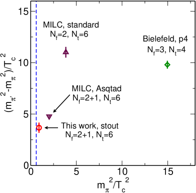
Figure 1: Pion mass splitting $\Delta_{\pi}=(m_{\pi}^{\prime 2}-m_{\pi}^{2})/T_{c}^{2}$ as a function of $(m_{\pi}/T_{c})^{2}$. The lattice spacings are the same as those at the finite temperature transition point. The mass of the Goldstone pion is denoted by $m_{\pi}$, that of the first non-Goldstone mode is by $m_{\pi}^{\prime}$. The horizontal blue line corresponds to the physical value of $(m_{\pi}/T_{c})^{2}$, where $T_{c}=173$MeV was assumed [21]. The taste violation of our stout-link improved action is much smaller than that of the unimproved action and even somewhat smaller than that of the asqtad action at the same $N_{t}$.

Isotropic lattice couplings are used, thus the lattice spacings are identical in all directions. The lattice action we used has the following form:

$$S = S_{g}+S_{f},$$ (1)

$$S_{g} = \sum_{x}\frac{\beta}{3}(c_{0}\sum_{\mu>\nu}W_{\mu,\nu}^{1\times 1}(x)+c_{1}\sum_{\mu\neq\nu}W_{\mu,\nu}^{1\times 2}(x)),$$ (2)

$$S_{f} = \sum_{x,y}\{\overline{\eta}_{ud}(x)[{D{/}}(U^{stout})_{xy}+m_{ud}\delta_{x,y}]^{-1/2}\eta_{ud}(y)$$ (3)

$$\mbox{\hskip 2.0pt}+\mbox{\hskip 2.0pt}\overline{\eta}_{s}(x)[{D{/}}(U^{stout})_{xy}+m_{s}\delta_{x,y}]^{-1/4}\eta_{s}(y)\},$$

where $W_{\mu,\nu}^{1\times 1}$, $W_{\mu,\nu}^{1\times 2}$ are real parts of the traces of the ordered products of link matrices along the $1\times 1$, $1\times 2$ rectangles in the $\mu$, $\nu$ plane. The coefficients satisfy $c_{0}+8c_{1}=1$ and $c_{1}=-1/12$ for the tree-level Symanzik improved action. $\eta_{ud}$ and $\eta_{s}$ are the pseudofermion fields for $u$, $d$ and $s$ quarks. ${D{/}}(U^{stout})$ is the four-flavor staggered Dirac matrix with stout-link improvement [10]. Let us also note here, that we use the 4th root trick in eq. (1), which might lead to problems of locality.

Our staggered action at a given $N_{t}$ yields the same limit for the pressure at infinite temperatures as the standard unimproved action. There are various techniques improving the high temperature scaling. However, usually an extrapolation based on $N_{t}$ and $N_{t}+2$ with standard staggered action gives a better high T behavior for the pressure than p4 [17] or asqtad [22, 23] action with $N_{t}$. Since our choice of action is about an order of magnitude faster than e.g. p4, we decided to use this less impoved action, with which our CPU resources made it possible to study two lattice spacings ($N_{t}$=4 and 6).

Staggered fermions have an unconvenient property: they violate taste symmetry at finite lattice spacing. Among other things this violation results in a splitting in the pion spectrum, which should vanish in the continuum limit. The stout-link improvement makes the staggered fermion taste symmetry violation small already at moderate lattice spacings. We found that a stout-smearing level of $N_{smr}$=2 and smearing parameter of $\rho$=0.15 are the optimal values of the smearing procedure. In order to illustrate the advantage of the stout-link action Figure 1 compares the taste violation in different approaches of the literature, which were used to determine the EoS of QCD. Results on the pion mass splitting for unimproved (used by Ref. [4, 5]) , p4 improved (used by Ref. [7, 24]), asqtad improved (used by [18, 25]) and stout-link improved (this work) staggered fermions are shown. The parameters were chosen to be the ones used by the different collaborations at the finite temperature transition point.

In previous staggered analyses the gauge configurations were produced by the R-algorithm [11] at a given stepsize. These studies were carried out usually at one stepsize, which is 1/2 or 2/3 of the light quark mass. The stepsize is an intrinsic parameter of the algorithm, which has to be extrapolated to zero. None of the previous staggered lattice thermodynamics studies performed this extrapolation. Using the R-algorithm without stepsize extrapolation leads to uncontrolled systematic errors. E.g. let us look at the difference (on $N_{t}$=6 lattices at intermediate $\beta$) between the extrapolated plaquette value and the value obtained at stepsize which is 2/3 of the light quark mass. This difference is larger than the total contribution of the plaquette to the pressure. Clearly, such a technique can not be used.

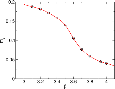
Figure 2: The line of constant physics. The result was obtained by using the $\phi$ and K masses (see text). The strange quark mass in lattice units is shown as a function of $\beta$. In the rest of our analysis we use light quark masses of $m_{ud}$=$m_{s}$/25.

Instead of using the approximate R-algorithm this work uses the exact RHMC-algorithm (rational hybrid Monte-Carlo) [12, 13]. This technique approximates the fractional powers of the Dirac operator by rational functions. Since the condition number of the Dirac operator changes as we change the mass, one should determine the optimal rational approximation for each quark mass. Note however, that this should be done only once, and the obtained parameters of these functions can be used in the entire configuration production. Our choices for the rational approximation were as good as few times the machine precision for the whole range of the eigenvalues of the Dirac operator.

Let us discuss the determination of the LCP. The LCP is defined as relationships between the bare lattice parameters ($\beta$ and lattice bare quark masses $m_{ud}$ and $m_{s}$). These relationships express that the physics (e.g. mass ratios) remains constant, while changing any of the parameters. It is important to emphasize that the LCP is unambiguous (independent of the physical quantities, which are used to define the above relationships) only in the continuum limit ($\beta\rightarrow\infty$). For our lattice spacings fixing some relationships to their physical values means that some other relationships will slightly deviate from the physical one. In thermodynamics the relevance of LCP comes into play when the temperature is changed by $\beta$ parameter. Then adjusting the mass parameters ($m_{ud}$ and $m_{s}$) is an important issue, neglecting this in simulations can lead to several % error in the EoS.

A particularly efficient (however only approximate, see later) way to obtain an LCP is by using simulations with three degenerate flavors with lattice quark mass $m_{q}$. The leading order chiral perturbation theory implies the mass relation for $s\bar{s}$ mesons. The strange quark mass is tuned accordingly, as

$$m_{PS}^{2}/m_{V}^{2}|_{m_{q}=m_{s}}=(2m_{K}^{2}-m_{\pi}^{2})/m_{\phi}^{2},$$ (4)

where $m_{PS}$ and $m_{V}$ are the pseudoscalar and vector meson masses in the simulations with three degenerate quarks. The light quark mass is calculated using the ratio $m_{ud}=m_{s}/25$ obtained by experimental mass input in the chiral perturbation theory [26]. We obtain $m_{s}(\beta)$ as shown in Figure 2.

Our approach using eq. (4) is appropriate if in the $n_{f}$=2+1 theory the vector meson mass depends only weakly on the light quark masses and the chiral perturbation theory for meson masses works upto the strange quark mass. After applying the LCP we cross-checked the obtained spectrum of the $n_{f}$=2+1 simulations. The resulting pseudoscalar (pion, kaon) and phi mass ratios agree with the experimental values on the 5–10% level. In dynamical simulations approximately 10% effect on $r_{0}$ is observed by changing the light quark masses from the strange mass to the physical limit. Thus, this slight mismatch of the spectrum results in a subdominant error on our overall scale, which is less or around 2%.

The determination of the EoS needs quite a few simulation points. Results are needed on finite temperature lattices ($N_{t}$=4 or 6) and on zero temperature lattices ($N_{t}\gg$ 4 or 6) at several $\beta$ values (we used 16 different $\beta$ values for $N_{t}$=4 and 14 values for $N_{t}$=6). Since our goal is to determine the EoS for physical quark masses we have to determine quantities in this small physical quark mass limit (we call these $\beta$ dependent bare light quark masses $m_{ud}(phys)$).

$\beta$	$m_{s}$	T=0	#	T$\neq$0	#	$\beta$	$m_{s}$	T=0	#	T$\neq$0	#
3.000	0.1938	163$\cdot$16	4	123$\cdot$4	9	3.450	0.1507	163$\cdot$32	29	183$\cdot$6	120
3.150	0.1848	163$\cdot$16	4	123$\cdot$4	9	3.500	0.1396	163$\cdot$32	33	183$\cdot$6	156
3.250	0.1768	163$\cdot$16	4	123$\cdot$4	9	3.550	0.1235	163$\cdot$32	30	183$\cdot$6	133
3.275	0.1742	163$\cdot$16	4	123$\cdot$4	9	3.575	0.1144	163$\cdot$32	28	183$\cdot$6	151
3.300	0.1713	163$\cdot$16	4	123$\cdot$4	9	3.600	0.1055	163$\cdot$32	31	183$\cdot$6	158
3.325	0.1683	163$\cdot$16	4	123$\cdot$4	9	3.625	0.0972	163$\cdot$32	33	183$\cdot$6	144
3.350	0.1651	163$\cdot$16	4	123$\cdot$4	9	3.650	0.0895	163$\cdot$32	30	183$\cdot$6	160
3.400	0.1583	163$\cdot$16	3	123$\cdot$4	9	3.675	0.0827	163$\cdot$32	32	183$\cdot$6	178
3.450	0.1507	163$\cdot$32	29	123$\cdot$4	9	3.700	0.0766	163$\cdot$32	33	183$\cdot$6	174
3.500	0.1396	163$\cdot$32	33	123$\cdot$4	9	3.750	0.0666	163$\cdot$32	35	183$\cdot$6	140
3.550	0.1235	163$\cdot$32	30	123$\cdot$4	9	3.800	0.0589	203$\cdot$40	26	183$\cdot$6	158
3.600	0.1055	163$\cdot$32	31	123$\cdot$4	9	3.850	0.0525	203$\cdot$40	23	183$\cdot$6	157
3.650	0.0895	163$\cdot$32	30	123$\cdot$4	9	3.930	0.0446	243$\cdot$48	6	183$\cdot$6	171
3.700	0.0766	163$\cdot$32	33	123$\cdot$4	9	4.000	0.0401	283$\cdot$56	4	183$\cdot$6	166
3.850	0.0525	203$\cdot$40	23	123$\cdot$4	9
4.000	0.0401	283$\cdot$56	4	123$\cdot$4	9

Table 1: Summary of our simulation points. For the physical light quark masses (we call them $m_{ud}(phys)$) 25 times smaller values were taken than for the strange mass. T$\neq$0 simulations were performed with the above $m_{s}$ and $\beta$ pairs, and at 5 different $m_{ud}$ values: {1,3,5,7,9}$\cdot m_{ud}(phys)$. T=0 simulations were performed with the above $m_{s}$ and $\beta$ pairs, but at 4 different $m_{ud}$ values: {3,5,7,9}$\cdot m_{ud}(phys)$. The total number of trajectories divided by 100 are collected in the # columns. The left column shows the $N_{t}$=4, whereas the right column shows the $N_{t}$=6 data. (For an explanation of our labeling see the text.)

For our finite temperature simulations ($N_{t}$=4,6) we used physical quark masses. The spatial sizes were always at least 3 times the temporal sizes. For the whole $\beta$ range on $N_{t}=4$ we checked that by increasing the $N_{s}/N_{t}$ ratio from 3 to 4 the results remained the same within our statistical uncertainties.

In the chirally broken phase (our zero temperature simulations, thus lattices for which $N_{t}\gg$ 4 or 6, belong always to this class) chiral perturbation theory can be used to extrapolate by a controlled manner to the physical light quark masses. Therefore for most of our simulation points we used four pion masses ($m_{\pi}\approx$235, 300, 355 and 405 MeV), which were somewhat larger than the physical one. (To simplify our notation in the rest of this paper we label these points as 3,5,7 and 9 times $m_{ud}(phys)$.) It turns out that the chiral condensates at all the four points can be fitted by linear function of pion mass squared with good $\chi^{2}$. (Later we will show, that only the chiral condensate is to be extrapolated to get the EoS at the physical quark mass.) The volumes were chosen in a way, that for three out of these four quark masses the spatial extentions of the lattices were approximately equal or larger than four times the correlation lengths of the pion channel. We checked for a few $\beta$ values that increasing the spatial and/or temporal extensions of the lattices results in the same expectation values within our statistical uncertainties. (For 3$\cdot m_{ud}(phys)$ values the spatial lengths of the lattices were only three times the correlation length of the pion channel. However, excluding this point from the extrapolations, the results do not change.)

A detailed list of our simulation points at zero and at non-zero temperature lattices are summarized in Table 1.

3 Equation of state

In this section results for two sets of lattice spacings ($N_{t}$=4,6) for the pressure, energy density, entropy density, quark number susceptibilities and for the speed of sound are presented.

We shortly review the integral technique to obtain the pressure [20]. For large homogeneous systems the pressure is proportional to the logarithm of the partition function:

$$pa^{4}=\frac{Ta}{V/a^{3}}\log Z(T,V)=\frac{1}{N_{t}N_{s}^{3}}\log Z(N_{s},N_{t};\beta,m_{q}).$$ (5)

(Index ‘q’ refers to the ${ud}$ and $s$ flavors.) The volume and temperature are connected to the spatial and temporal extensions of the lattice:

$$V=(N_{s}a)^{3}, T=\frac{1}{N_{t}a}.$$ (6)

The divergent zero-point energy has to be removed by subtracting the zero temperature ($N_{t}\to\infty$) part of eq. (5). In practice the zero temperature subtraction is performed by using lattices with finite, but large $N_{t}$ (called $N_{t0}$, see Table 1). So the normalized pressure becomes:

$$\frac{p}{T^{4}}=N_{t}^{4}\left[\frac{1}{N_{t}N_{s}^{3}}\log Z(N_{s},N_{t};\beta,m_{q})-\frac{1}{N_{t0}N_{s0}^{3}}\log Z(N_{s0},N_{t0};\beta,m_{q})\right].$$ (7)

With usual Monte-Carlo techniques one cannot measure $\log Z$ directly, but only its derivatives with respect to the bare parameters of the lattice action. Having determined the partial derivatives one integrates in the multi-dimensional parameter space:

$$\frac{p}{T^{4}}=N_{t}^{4}\int^{(\beta,m_{q})}_{(\beta_{0},m_{q0})}d(\beta,m_{q})\left[\frac{1}{N_{t}N_{s}^{3}}\left(\begin{array}[]{c}{\partial\log Z}/{\partial\beta}\\ {\partial\log Z}/{\partial m_{q}}\end{array}\right)-\frac{1}{N_{t0}N_{s0}^{3}}\left(\begin{array}[]{c}{\partial\log Z_{0}}/{\partial\beta}\\ {\partial\log Z_{0}}/{\partial m_{q}}\end{array}\right)\right],$$ (8)

where $Z/Z_{0}$ are shorthand notations for $Z(N_{s},N_{t})/Z(N_{s0},N_{t0})$. Since the integrand is a gradient, the result is by definition independent of the integration path. We need the pressure along the LCP, thus it is convenient to measure the derivatives of $\log Z$ along the LCP and perform the integration over this line in the $\beta$, $m_{ud}$ and $m_{s}$ parameter space. The lower limits of the integrations (indicated by $\beta_{0}$ and $m_{q0}$) were set sufficiently below the transition point. By this choice the pressure gets independent of the starting point (in other words it vanishes at small temperatures). In the case of $2+1$ flavor staggered QCD the derivatives of $\log Z$ with respect to $\beta$ and $m_{q}$ are proportional to the expectation value of the gauge action ($\langle S_{g}\rangle$ c.f. eq. (1)) and to the chiral condensates ($\langle\bar{\psi}\psi_{q}\rangle$), respectively. Eq. (8) can be rewritten appropriately and the pressure is given by (in this formula we write out explicitely the flavours):

$$\frac{p}{T^{4}}=N_{t}^{4}\int^{(\beta,m_{ud},m_{s})}_{(\beta_{0},m_{ud0},m_{s0})}d(\beta,m_{ud},m_{s})\left[\frac{1}{N_{t}N_{s}^{3}}\left(\begin{array}[]{c}\langle{\rm-S_{g}/\beta}\rangle\\ \langle\bar{\psi}\psi_{ud}\rangle\\ \langle\bar{\psi}\psi_{s}\rangle\end{array}\right)-\frac{1}{N_{t0}N_{s0}^{3}}\left(\begin{array}[]{c}\langle{\rm-S_{g}/\beta}\rangle_{0}\\ \langle\bar{\psi}\psi_{ud}\rangle_{0}\\ \langle\bar{\psi}\psi_{s}\rangle_{0}\end{array}\right)\right],$$ (9)

where $\langle\dots\rangle_{0}$ means averaging on a $N_{s0}^{3}\cdot N_{t0}$ lattice.

The integral method was originally introduced for the pure gauge case, for which the integral is one dimensional, it is performed along the $\beta$ axis. Previous studies for staggered dynamical QCD (e.g. [5, 27, 7]) used a one-dimensional parameter space instead of performing it along the LCP. Note, that for full QCD the integration should be performed along a LCP path in a multi-dimensional parameter space.

$N_{t}$	p/$T^{4}$	$c_{s}^{2}$	$\chi/T^{2}$
4	9.12	1/3	2.24
6	7.86	1/3	1.86
$\infty$	5.21	1/3	1

Table 2: Summary of the results for the 2+1 flavor pressure, speed of sound and 1 flavor quark number susceptibility in the non-interacting Stefan-Boltzmann limit. $\epsilon/T^{4}$ is 3 times, whereas $s/T^{3}$ is 4 times the normalized value of the pressure ($p/T^{4}$) in the Stefan-Boltzmann limit. The first two lines gives the results for $N_{t}$=4,6 and the third line contains the results in the continuum (in the thermodynamic limit).

Using appropriate thermodynamical relations one can obtain any thermal properties of the system. For example the energy density ($\epsilon$), entropy density ($s$) and speed of sound ($c_{s}^{2}$) can be derived as

$$\epsilon=T(\partial p/\partial T)-p, s=(\epsilon+p)T, c_{s}^{2}=\frac{dp}{d\epsilon}.$$ (10)

To be able to do theses derivatives one has to know the temperature along the LCP. Since the temperature is connected to the lattice spacing as $T=(N_{t}a)^{-1},$ we need a reliable estimate on $a$. The lattice spacings at different points of the LCP are determined by first matching the static potentials for different $\beta$ values at an intermediate distance for $m_{ud}=\{3,5\}m_{ud}(phys)$ quark masses, then extrapolating the results to the physical quark mass. Relating these distances to physical observables (determining the overall scale in physical units) will be the topic of a subsequent publication. We show the results as a function of $T/T_{c}$. The transition temperature ($T_{c}$) is defined by the inflection point of the isospin number susceptibility ($\chi_{I}$, see later).

To get the energy density the literature usually uses another quantity, namely $\epsilon$-3$p$, which can be also directly measured on the lattice. In our analysis it turned out to be more appropriate to calculate first the pressure directly from the raw lattice data (eq. (9)) and then determine the energy density and other quantities from the pressure (eq. (10)). The reasons for that can be summarized as follows. As we discussed we perform T$\neq$0 simulations with physical quark masses, whereas the subtraction terms from T=0 simulations are extrapolated from larger quark masses. This sort of extrapolation is adequate for the chiral condensates, for which chiral perturbation techniques work well. Thus, one can choose an integration path for the T=0 part of the pressure, which moves along a LCP at some larger $m_{ud}$ (e.g. 9 times $m_{ud}(phys)$) and then at fixed $\beta$ goes down to the physical quark mass. No comparable analogous technique is available for the combination $\epsilon$-3$p$.

We have also calculated the pressure for the larger quark masses. Plotting it as a function of the temperature the differences between them are significant. As a function of $T/T_{c}$ these differences are smaller, but still remain statistically significant in the $1.2...2.0T_{c}$ region. Note that statements on the mass dependence are only qualitative since such an analysis requires the careful matching of the scales at different quark masses. It is non-trivial and will be the topic of a forthcoming paper.

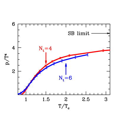
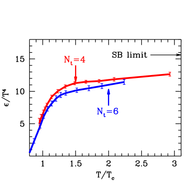
Figure 3: a.) The left panel shows the pressure $p$, as a function of the temperature. Both $N_{t}$=4 (red, upper curve) and $N_{t}$=6 (blue, lower curve) data are obtained along the LCP. They are normalized by $T^{4}$ and scaled by $c_{cont}/c_{N_{t}}$ (see text and Table 2). In order to lead the eye lines connect the data points. b.) The right panel is the energy density ($\epsilon$), red (upper) and blue (lower) for $N_{t}$=4 and 6 respectively. This result was obtained directly from the pressure.

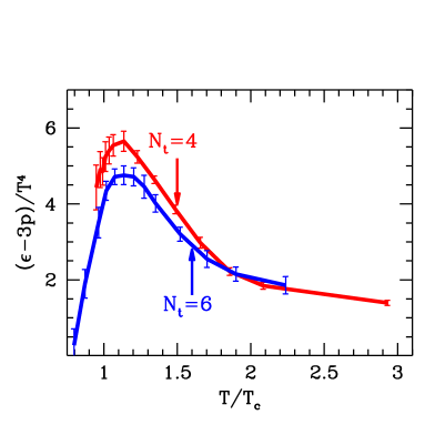
Figure 4: The interaction measure, the values are normalized by $c_{cont}/c_{N_{t}}$ of the energy density. The labeling is the same as for Figure 3.

Let us present the results. In order to show how the different quantities scale with the lattice spacing we show always $N_{t}$=4,6 results on the same plot. In addition, in order to make the relationship with the continuum limit more transparent we multiply the raw lattice results at finite temporal extensions ($N_{t}$=4,6) with $c_{cont}/c_{N_{t}}$, where the c values are the results in the free non-interacting plasma (Stefan-Boltzmann limit). These c values are summarized in Table 2 for the pressure, speed of sound, and for the quark number susceptibility at $N_{t}$=4,6 and in the continuum limit. By this multiplication the lattice thermodynamic quantities should approach the continuum Stefan-Boltzmann values for extreme large temperatures.

Table 3 contains our most important numerical results. We tabulated the raw and normalized pressure values for both lattice spacings and for all of our simulation points. This data set and eq. (10) were used to obtain the following figures. Figure 3 shows the equation of state on $N_{t}$=4,6 lattices. The pressure (left panel) and $\epsilon$ (right panel) are presented as a function of the temperature. The Stefan-Boltzmann limit is also shown. On Figure 4 the interaction measure (i.e. $(\epsilon-3p)/T^{4}$) is plotted, it is normalized by the corresponding $c_{cont}/c_{N_{t}}$ value of the energy density. Figure 5 shows the entropy density (left panel) and the speed of sound (right panel), which can be obtained by using the pressure and energy density data (c.f. $sT$=$\epsilon$+$p$ and $c_{s}^{2}$=$dp$/$d\epsilon$) of the previous Figure 3. Clearly, the uncertainties of the pressure and those of the energy density cumulate in the speed of sound, therefore it is less precisely determined.

$\beta$	$T/T_{c}$	$p/T^{4}$ (raw)	$p/T^{4}$ (scaled)	$\beta$	$T/T_{c}$	$p/T^{4}$ (raw)	$p/T^{4}$ (scaled)
3.000	$0.90$	$0.12(0.02)$	$0.07(0.01)$	3.450	$0.80$	$0.07(0.11)$	$0.05(0.08)$
3.150	$0.95$	$0.32(0.07)$	$0.19(0.04)$	3.500	$0.87$	$0.23(0.11)$	$0.15(0.08)$
3.250	$0.98$	$0.59(0.10)$	$0.34(0.06)$	3.550	$0.96$	$0.59(0.12)$	$0.39(0.08)$
3.275	$0.99$	$0.73(0.10)$	$0.42(0.06)$	3.575	$1.02$	$0.91(0.12)$	$0.60(0.08)$
3.300	$1.01$	$0.91(0.10)$	$0.52(0.06)$	3.600	$1.07$	$1.29(0.13)$	$0.86(0.08)$
3.325	$1.04$	$1.13(0.10)$	$0.65(0.06)$	3.625	$1.14$	$1.69(0.13)$	$1.12(0.09)$
3.350	$1.06$	$1.39(0.09)$	$0.79(0.05)$	3.650	$1.20$	$2.10(0.14)$	$1.40(0.09)$
3.400	$1.14$	$2.04(0.10)$	$1.16(0.06)$	3.675	$1.28$	$2.51(0.14)$	$1.66(0.10)$
3.450	$1.23$	$2.79(0.10)$	$1.59(0.06)$	3.700	$1.35$	$2.88(0.15)$	$1.91(0.10)$
3.500	$1.34$	$3.56(0.11)$	$2.04(0.07)$	3.750	$1.52$	$3.50(0.15)$	$2.32(0.10)$
3.550	$1.49$	$4.32(0.12)$	$2.47(0.07)$	3.800	$1.70$	$3.99(0.16)$	$2.65(0.11)$
3.600	$1.66$	$4.96(0.12)$	$2.83(0.07)$	3.850	$1.90$	$4.36(0.16)$	$2.89(0.11)$
3.650	$1.86$	$5.46(0.12)$	$3.12(0.07)$	3.930	$2.24$	$4.82(0.17)$	$3.19(0.11)$
3.700	$2.09$	$5.84(0.12)$	$3.34(0.07)$	4.000	$2.55$	$5.14(0.17)$	$3.41(0.11)$
3.850	$2.93$	$6.57(0.15)$	$3.75(0.09)$
4.000	$3.93$	$6.97(0.16)$	$3.98(0.09)$

Table 3: Numerical values of the pressure for all of our simulation points. The left column shows the $N_{t}$=4, whereas the right column shows the $N_{t}$=6 data. Both the raw values and the ones scaled by $c_{cont}/c_{N_{t}}$ are given.

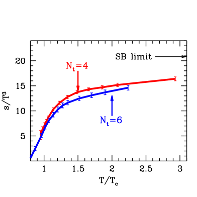
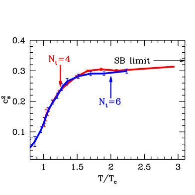
Figure 5: The entropy density (left panel, normalized by $T^{3}$) and the speed of sound (right panel). The labeling is the same as for Figure 3.

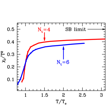
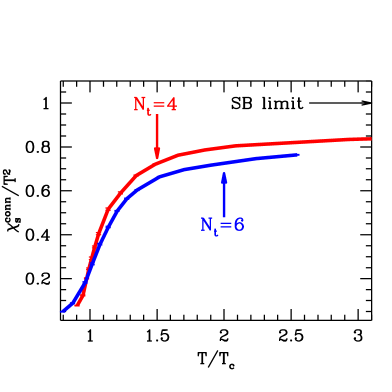
Figure 6: The isospin susceptibility (left panel, normalized by $T^{2}$) and the connected part of the strangeness susceptibility (right panel, normalized by $T^{2}$). The labeling is the same as for Figure 3.

Light and strange quark number susceptibilities ($\chi_{ud}$ and $\chi_{s}$) are defined via [28]

$$\frac{\chi_{q}}{T^{2}}=\frac{N_{t}}{N_{s}^{3}}\left.\frac{\partial^{2}\log Z}{\partial\mu_{q}^{2}}\right|_{\mu_{q}=0},$$ (11)

where $\mu_{ud}$ and $\mu_{s}$ are the light and strange quark chemical potentials (in lattice units). With the help of the quark number operators

$$Q_{q}=\frac{1}{4}\frac{\partial}{\partial\mu_{q}}\log\det({D{/}}+m_{q}),$$

the susceptibilities can be written as

$$\frac{\chi_{q}}{T^{2}}=\frac{N_{t}}{N_{s}^{3}}\left(\langle Q_{q}^{2}\rangle_{\mu_{q}=0}+\left\langle\frac{\partial Q_{q}}{\partial\mu_{q}}\right\rangle_{\mu_{q}=0}\right).$$

The first term is usually referred as disconnected, the second as connected part. The connected part of the light quark number susceptibility is 2 times the susceptibility of the isospin number ($\chi_{I}$). It is presented on the left panel of Figure 6. For our statistics and evaluation method the disconnected parts are all consistent with zero and their value is far smaller than those of the connected parts. The right panel of Figure 6 contains the connected part of the strange number susceptibility.

4 Summary, conclusion

In this letter we presented results of a large scale numerical lattice study on the thermodynamics of QCD.

We determined the equation of state. Our analysis attempted to improve on existing analyses by several means. We used for the lightest hadronic degree of freedom the physical pion mass. We used finer lattices with two different sets of lattice spacings ($N_{t}$=4,6). We kept our system on the line of constant physics (LCP) instead of changing the physics with the temperature. Due to our smaller lattice spacing and particularly due to our stout-link improved fermionic action the unphysical pion mass splitting was much smaller than in any previous analysis. We used an exact calculation algorithm instead of an approximate one. Our scale was determined by a theoretically sound quantity and not based on the string tension.

We presented results for the pressure, energy density, entropy density, speed of sound and on the isospin and strangeness susceptibilities.

Since the finite lattice spacing effects are quite different for different temperatures a reliable continuum estimate can only be given if results on an even finer lattice ($N_{t}$=8) were obtained. This sort of analysis would be a major step towards the final results for the equation of state.

Acknowledgments We thank Claude Bernard and Carleton DeTar for providing the pion splitting value from the MILC Asqtad result. This research was partially supported by OTKA Hungarian Science Grants No. T34980, T37615, M37071, T032501, AT049652, and by DFG German Research Grant No. FO 502/1-1. This research is part of the EU Integrated Infrastructure Initiative Hadronphysics project under contract number RII3-CT-20040506078. The computations were carried out at Eötvös University on the 330 processor PC cluster of the Institute for Theoretical Physics and the 1024 processor PC cluster of Wuppertal University, using a modified version of the publicly available MILC code [29] and a next-neighbour communication architecture [30].

References

- [1] G. Boyd et al., Thermodynamics of su(3) lattice gauge theory, Nucl. Phys. B469 (1996) 419–444, [hep-lat/9602007].
- [2] CP-PACS Collaboration, M. Okamoto et al., Equation of state for pure su(3) gauge theory with renormalization group improved action, Phys. Rev. D60 (1999) 094510, [hep-lat/9905005].
- [3] CP-PACS Collaboration, Y. Namekawa et al., Thermodynamics of su(3) gauge theory on anisotropic lattices, Phys. Rev. D64 (2001) 074507, [hep-lat/0105012].
- [4] T. Blum, L. Karkkainen, D. Toussaint, and S. A. Gottlieb, The beta function and equation of state for qcd with two flavors of quarks, Phys. Rev. D51 (1995) 5153–5164, [hep-lat/9410014].
- [5] MILC Collaboration, C. W. Bernard et al., The equation of state for two flavor qcd at n(t) = 6, Phys. Rev. D55 (1997) 6861–6869, [hep-lat/9612025].
- [6] CP-PACS Collaboration, A. Ali Khan et al., Equation of state in finite-temperature qcd with two flavors of improved wilson quarks, Phys. Rev. D64 (2001) 074510, [hep-lat/0103028].
- [7] F. Karsch, E. Laermann, and A. Peikert, The pressure in 2, 2+1 and 3 flavour qcd, Phys. Lett. B478 (2000) 447–455, [hep-lat/0002003].
- [8] Z. Fodor, S. D. Katz, and K. K. Szabo, The qcd equation of state at nonzero densities: Lattice result, Phys. Lett. B568 (2003) 73–77, [hep-lat/0208078].
- [9] F. Csikor et al., Equation of state at finite temperature and chemical potential, lattice qcd results, JHEP 05 (2004) 046, [hep-lat/0401016].
- [10] C. Morningstar and M. J. Peardon, Analytic smearing of su(3) link variables in lattice qcd, Phys. Rev. D69 (2004) 054501, [hep-lat/0311018].
- [11] S. A. Gottlieb, W. Liu, D. Toussaint, R. L. Renken, and R. L. Sugar, Hybrid molecular dynamics algorithms for the numerical simulation of quantum chromodynamics, Phys. Rev. D35 (1987) 2531–2542.
- [12] M. A. Clark, B. Joo, and A. D. Kennedy, Comparing the r algorithm and rhmc for staggered fermions, Nucl. Phys. Proc. Suppl. 119 (2003) 1015–1017, [hep-lat/0209035].
- [13] M. A. Clark and A. D. Kennedy, The rhmc algorithm for 2 flavors of dynamical staggered fermions, Nucl. Phys. Proc. Suppl. 129 (2004) 850–852, [hep-lat/0309084].
- [14] SESAM Collaboration, G. S. Bali, H. Neff, T. Duessel, T. Lippert, and K. Schilling, Observation of string breaking in qcd, Phys. Rev. D71 (2005) 114513, [hep-lat/0505012].
- [15] R. Sommer, A new way to set the energy scale in lattice gauge theories and its applications to the static force and alpha-s in su(2) yang-mills theory, Nucl. Phys. B411 (1994) 839–854, [hep-lat/9310022].
- [16] C. Aubin et al., Light hadrons with improved staggered quarks: Approaching the continuum limit, Phys. Rev. D70 (2004) 094505, [hep-lat/0402030].
- [17] U. M. Heller, F. Karsch, and B. Sturm, Improved staggered fermion actions for qcd thermodynamics, Phys. Rev. D60 (1999) 114502, [hep-lat/9901010].
- [18] C. Bernard et al., The equation of state for qcd with 2+1 flavors of quarks, hep-lat/0509053.
- [19] C. Jung, Thermodynamics using p4-improved staggered fermion action on qcdoc, hep-lat/0510035.
- [20] J. Engels, J. Fingberg, F. Karsch, D. Miller, and M. Weber, Nonperturbative thermodynamics of su(n) gauge theories, Phys. Lett. B252 (1990) 625–630.
- [21] F. Karsch, E. Laermann, and A. Peikert, Quark mass and flavor dependence of the qcd phase transition, Nucl. Phys. B605 (2001) 579–599, [hep-lat/0012023].
- [22] G. P. Lepage, Flavor-symmetry restoration and symanzik improvement for staggered quarks, Phys. Rev. D59 (1999) 074502, [hep-lat/9809157].
- [23] MILC Collaboration, K. Orginos, D. Toussaint, and R. L. Sugar, Variants of fattening and flavor symmetry restoration, Phys. Rev. D60 (1999) 054503, [hep-lat/9903032].
- [24] A. Peikert, Qcd thermodynamics with 2+1 quark flavours in lattice simulations, Thesis, Univ. Bielefeld (2000).
- [25] C. Bernard and C. DeTar, private communication.
- [26] J. Gasser and H. Leutwyler, Chiral perturbation theory: Expansions in the mass of the strange quark, Nucl. Phys. B250 (1985) 465.
- [27] J. Engels et al., Thermodynamics of four-flavour qcd with improved staggered fermions, Phys. Lett. B396 (1997) 210–216, [hep-lat/9612018].
- [28] MILC Collaboration, C. Bernard et al., Qcd thermodynamics with three flavors of improved staggered quarks, Phys. Rev. D71 (2005) 034504, [hep-lat/0405029].
- [29] MILC Collaboration, public lattice gauge theory code, see http://physics.indiana.edu/~sg/milc.html.
- [30] Z. Fodor, S. D. Katz, and G. Papp, Better than $1/mflops sustained: A scalable pc-based parallel computer for lattice qcd, Comput. Phys. Commun. 152 (2003) 121–134, [hep-lat/0202030].