The finite temperature QCD using 2+1 flavors of domain wall fermions at $\boldmath{N_{t}=8}$

Abstract

We study the region of the QCD phase transition using 2+1 flavors of domain wall fermions (DWF) and a $16^{3}\times 8$ lattice volume with a fifth dimension of $L_{s}=32$. The disconnected light quark chiral susceptibility, quark number susceptibility and the Polyakov loop suggest a chiral and deconfining crossover transition lying between 155 and 185 MeV for our choice of quark mass and lattice spacing. In this region the lattice scale deduced from the Sommer parameter $r_{0}$ is $a^{-1}\approx 1.3$ GeV, the pion mass is $\approx 300$ MeV and the kaon mass is approximately physical. The peak in the chiral susceptibility implies a pseudo critical temperature $T_{c}=171(10)(17)$ MeV where the first error is associated with determining the peak location and the second with our unphysical light quark mass and non-zero lattice spacing. The effects of residual chiral symmetry breaking on the chiral condensate and disconnected chiral susceptibility are studied using several values of the valence $L_{s}$.

I Introduction

The properties of strongly-interacting matter change dramatically as the temperature is increased. At a sufficiently high temperature, the basic constituents of matter (quarks and gluons) are no longer confined inside hadronic bound states, but exist as a strongly interacting quark-gluon plasma (QGP). The properties of the QGP have been subject to significant theoretical and experimental study. The physics of the transition region controls the initial formation of the QGP in a heavy-ion collision, as well as the details of hadronic freeze-out as the QGP expands and cools. Thus, the transition temperature and the order of the transition are of fundamental importance in their own right and of particular interest to both the theoretical and experimental heavy-ion community.

The location and nature of the QCD phase transition has been extensively studied using lattice techniques with several different fermion actions Bazavov:2009zn ; Cheng:2006qk ; Bernard:2004je ; Aoki:2006br ; Chen:2000zu ; Bornyakov:2009qh . Recently, the most detailed studies of the transition temperature have been performed with different variants of the staggered fermion action Bazavov:2009zn ; Cheng:2006qk ; Bernard:2004je ; Aoki:2006br . Although staggered fermions are computationally inexpensive, they suffer the disadvantage that they do not preserve the full SU(2)$\times$SU(2) chiral symmetry of continuum QCD, but only a $U(1)$ subgroup. This lack of chiral symmetry is immediately apparent in the pion spectrum for staggered quarks, where there is only a single pseudo-Goldstone pion, while the other pions acquire additional mass from $O(a^{2})$ flavor mixing terms in the action.

Thus, it is important to study the QCD phase transition using a different fermion discretization scheme. The Wilson fermion formulation is fundamentally different from the staggered approach and would be an obvious basis for an alternative approach. However, Wilson fermions may be a poor alternative because in that formulation chiral symmetry is completely broken at the lattice scale and only restored in the continuum limit, the same limit in which the breaking of SU(2)$\times$SU(2) chiral symmetry in the staggered fermion formulation disappears.

A particularly attractive fermion formulation to employ is that of domain wall fermions Kaplan:1992bt ; Shamir:1993zy ; Furman:1994ky . This is a variant of Wilson fermions in which a fifth dimension is introduced (the $s$ direction). In this scheme, left and right-handed chiral states are bound to the four dimensional boundaries of the five-dimensional volume. The finite separation, $L_{s}$ between the left- and right-hand boundaries or walls allows some mixing between these left- and right-handed modes giving rise to a residual chiral symmetry breaking. However, in contrast to Wilson fermions, this residual chiral symmetry breaking can be strongly suppressed by taking the fifth-dimensional extent ($L_{s}$) to be large.

To leading order in an expansion in lattice spacing, the residual chiral symmetry breaking can be characterized by a single parameter, the residual mass $m_{\mathrm{res}}$, which acts as an additive shift to the bare input quark mass. Thus, the full continuum SU(2)$\times$SU(2) chiral symmetry can be reproduced to arbitrary accuracy by choosing $L_{s}$ sufficiently large, even at finite lattice spacing. However, this good control of chiral symmetry breaking comes with an approximate factor of $L_{s}$ increase in computational cost.

For these reasons, one of the first applications of the domain wall fermion approach was to the study of QCD thermodynamics using lattices with a time extent of $N_{t}=4$ and 6 Chen:2000zu . These early results were quite encouraging, showing a clear signal for a physical, finite temperature transition. However, these were two-flavor calculations limited to quarks with relatively heavy masses on the order of that of the strange quark and with such large lattice spacings that higher order residual chiral symmetry breaking effects, beyond $m_{\mathrm{res}}\neq 0$, may have been important.

Given the substantial increase in computer capability and the deeper understanding of domain wall fermions that has been achieved over the past decade, it is natural to return to this approach. Now significantly smaller quark masses and much finer lattices with $N_{t}=8$ can be studied and important aspects of residual chiral symmetry breaking can be recognized and explored.

This paper presents such a first study of the QCD finite temperature transition region using domain wall fermions at $N_{t}=8$ and is organized as follows. Section II gives the details of our simulation, with regard to the choice of actions, simulation parameters, and algorithms. Section III presents our results for finite-temperature observables such as the chiral condensate, chiral susceptibility, quark number susceptibility, Polyakov loop, and Polyakov loop susceptibility. Section IV gives results for the zero-temperature observables: the static quark potential and the hadron spectrum, that were calculated to determine the lattice spacing and quark masses in physical units. Section V discusses the effects of residual chiral symmetry breaking on our calculation and consistency checks of this finite temperature application of the domain wall method. Section VI makes an estimate of the pseudo critical temperature $T_{c}$ which characterizes the critical region and its associated systematic errors. Finally, Section VII presents our conclusions and outlook for the future.

II Simulation Details

For our study we utilize the standard domain wall fermion action and the Iwasaki gauge action. The properties of this combination of actions has been extensively studied at zero temperature by the RBC-UKQCD collaboration Antonio:2006px ; Allton:2007hx ; Bernard:2000gd ; Allton:2008pn .

Using the data from Ref. Antonio:2006px ; Allton:2007hx ; Antonio:2008zz ; Allton:2008pn , we extrapolated to stronger coupling in order to estimate the bare input parameters: the gauge coupling, input light quark mass, and input strange quark mass ($\beta$, $m_{l}$, $m_{s}$), appropriate for the region of the finite-temperature transition at $N_{t}=8$. The value of the critical gauge coupling was estimated to be $\beta_{c}\sim 2.00$ and the corresponding residual mass $m_{\mathrm{res}}\sim 0.008$ for $L_{s}=32$. As a result, we have used $m_{l}=0.003$ and $m_{s}=0.037$ for the input light and strange quark masses in all of our runs. This corresponds to $(m_{l}+m_{\mathrm{res}})/(m_{s}+m_{\mathrm{res}})\approx 0.25$.

For the finite temperature ensembles, we have used a lattice volume of $16^{3}\times 8$, with $L_{s}=32$. Table 1 shows the different values of $\beta$ that we chose, as well as the total number of molecular dynamics trajectories generated for each $\beta$. In the immediate vicinity of the transition, we have approximately $2000-3000$ trajectories, with fewer trajectories as we move further away from the critical gauge coupling, $\beta_{c}$.

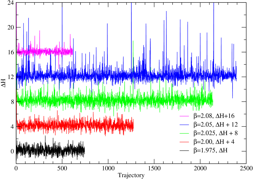
Figure 1: The time history of $\Delta H$ for selected values of $\beta$. There is a vertical offset of 4 units between successive data sets with the lowest data set unshifted.

We use the rational hybrid Monte Carlo (RHMC) algorithm Clark:2004cp ; Clark:2006fx to generate the dynamical field configurations. An Omelyan integrator deForcrand:2006pv ; Takaishi:2005tz with $\lambda=0.22$ was used to numerically integrate the molecular dynamics trajectory. A three-level integration scheme was used, where the force from the gauge fields was integrated with the finest time-step. The ratio of the determinant of three flavors of strange quark to the determinant of three flavors of Pauli-Villars bosons was included at the intermediate time-step, while the ratio of the determinant of the two light quarks and the determinant of two strange pseudoquarks was integrated with the largest step-size. The molecular dynamics trajectories were of unit length ($\tau=1$), with a largest step size of $\delta\tau=0.2$ or $\delta\tau=0.167$. This allowed us to achieve an acceptance rate of approximately $75\%$. Table 1 summarizes the parameters that we have used for the finite temperature ensembles, as well as important characteristics of the RHMC evolution. Figure 1 shows the time history for $\Delta\mathcal{H}$ at a few selected gauge couplings.

We also generated 1200 trajectories at $\beta=2.025$ with a volume of $16^{3}\times 32$ and $L_{s}=32$, also with $m_{l}=0.003$ and $m_{s}=0.037$. We used these zero temperature configurations to determine the meson spectrum, as well as the static quark potential.

$\beta$	1.95	1.975	2.00	2.0125	2.025	2.0375	2.05	2.0625	2.08	2.11	2.14
Trajectories	745	1100	1275	2150	2210	2690	3015	2105	1655	440	490
Acceptance Rate	0.778	0.769	0.760	0.776	0.745	0.746	0.754	0.753	0.852	0.875	0.859
$\sqrt{\langle\Delta\mathcal{H}^{2}\rangle}$	0.603	0.583	0.647	0.687	0.824	1.072	1.248	1.599	0.478	0.472	0.345
$\langle\exp(-\Delta\mathcal{H})\rangle$	1.026	1.022	0.969	1.017	0.987	0.995	0.987	1.051	1.002	1.010	0.9979

Table 1: Values for $\beta$, numbers of trajectories accumulated, results for the rms shift in the RHMC Hamiltonian and the average exponentiated Hamiltonian shift (which should be unity). All runs were carried out with a trajectory length of 1 and an outer step size of 0.2 except for the case of $\beta=2.08$ where $\delta\tau=0.167$ was used.

III Finite temperature observables

For QCD with massless quarks, there is a true phase transition from a low-temperature phase with spontaneous chiral symmetry breaking to a high temperature phase where chiral symmetry is restored. If the quarks have a finite mass ($m_{f}$), that explicitly breaks chiral symmetry, the existence of a chiral phase transition persists for masses up to a critical quark mass, $m_{f}<m_{f}^{\mathrm{crit}}$, above which the theory undergoes a smooth crossover rather than a singular phase transition as the temperature is varied. The value of $m_{f}^{\mathrm{crit}}$ is poorly known and depends sensitively on the number of light quark flavors. For a transition region dominated by two light quark flavors $m_{f}^{\mathrm{crit}}$ is expected to vanish and the transition to be second order only for massless quarks. For three or more light flavors a first order region $0\leq m_{f}<m_{f}^{\mathrm{crit}}$ should be present.

III.1 Chiral condensate

The order parameter that best describes the chiral phase transition is the chiral condensate, $\langle\overline{\psi}_{q}\psi_{q}\rangle$, which vanishes in the symmetric phase, but attains a non-zero expectation value in the chirally broken phase. For quark masses above $m_{f}^{\mathrm{crit}}$, the chiral condensate will show only analytic behavior, but both the light and strange quark chiral condensates, $\langle\overline{\psi}_{l}\psi_{l}\rangle,\langle\overline{\psi}_{s}\psi_{s}\rangle$, and the disconnected part of their chiral susceptibilities, $\chi_{l},\chi_{s}$, still contain information about the chiral properties of the theory in the vicinity of the crossover transition. The chiral condensate and the disconnected chiral susceptibility for a single quark flavor are defined as:

$$\frac{\langle\overline{\psi}_{q}\psi_{q}\rangle}{T^{3}} = \frac{1}{VT^{2}}\frac{\partial\ln Z}{\partial m_{q}}=\frac{N_{t}^{2}}{N_{s}^{3}}\langle\mathrm{Tr}M_{q}^{-1}\rangle$$ (1)

$$\frac{\chi_{q}}{T^{2}} = \frac{1}{VT}\langle\left(\mathrm{Tr}M_{q}^{-1}\right)^{2}-\langle\mathrm{Tr}M_{q}^{-1}\rangle^{2}\rangle=VT^{3}\langle\left(\overline{\psi}_{q}\psi_{q}\right)^{2}-\langle\overline{\psi}_{q}\psi_{q}\rangle^{2}\rangle$$ (2)

where $m_{q}$ is the mass of the single quark $q$ being examined, $T$ the temperature, $V$ the spatial volume and $N_{t}$ and $N_{s}$ are the number of lattice sites in the temporal and spatial directions, respectively.

On our finite temperature ensembles, we calculate both the light ($m_{l}=0.003$) and strange ($m_{s}=0.037$) chiral condensates using 5 stochastic sources to estimate $\langle\overline{\psi}_{q}\psi_{q}\rangle$ on every fifth trajectory. Using multiple stochastic sources on a given configuration allows us to extract an unbiased estimate of the fluctuations in $\overline{\psi}_{q}\psi_{q}$ and to calculate the disconnected chiral susceptibility. The Polyakov loop is calculated after every trajectory.

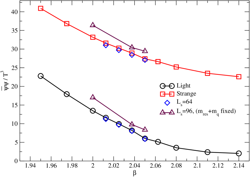
Figure 2: Unitary values for $\langle\overline{\psi}_{l}\psi_{l}\rangle$ and $\langle\overline{\psi}_{s}\psi_{s}\rangle$ (the circles and squares respectively) for $L_{s}=32$, as well as additional measurements with $L_{s}=64$ and $L_{s}=96$ for the valence quarks. For the $L_{s}=96$ measurements, $m_{l}$ and $m_{s}$ are adjusted so that values for the sum $m_{q}+m_{res}$ are approximately the same as those for $L_{s}=32$.

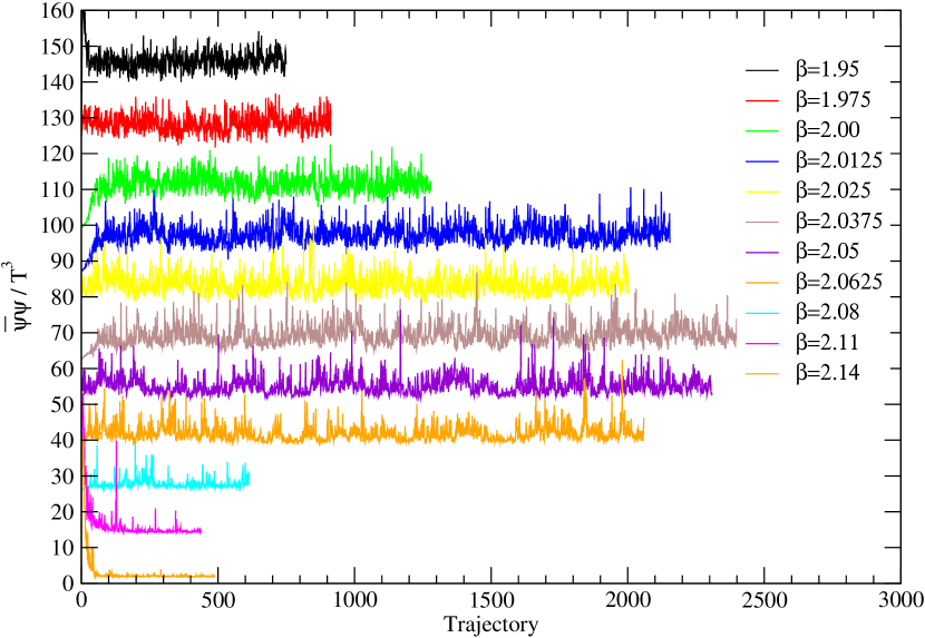
Figure 4: The time history of $\overline{\psi}_{l}\psi_{l}$ for the light quarks. There is a vertical offset of approximately 12 units between successive data sets with the lowest set unshifted.

Figures 2 and 3 show the chiral condensate and the disconnected part of the chiral susceptibility, respectively. Examining the light and strange quark chiral condensates, it is difficult to precisely determine an inflection point. Such an inflection point could be used to locate the mid-point of a thermal crossover. We can also study the disconnected chiral susceptibility. This is computed from the fluctuations in the chiral condensate and will show a peak near the location of the inflection point of the chiral condensate. Examining the time history of $\overline{\psi}_{l}\psi_{l}$ shown in Fig. 4, one can see that the fluctuations have a strong $\beta$ dependence. We will identify the peak in these fluctuations with the location of the chiral crossover. The chiral susceptibility shown in Fig. 3, has a clear peak near $\beta=2.0375$.

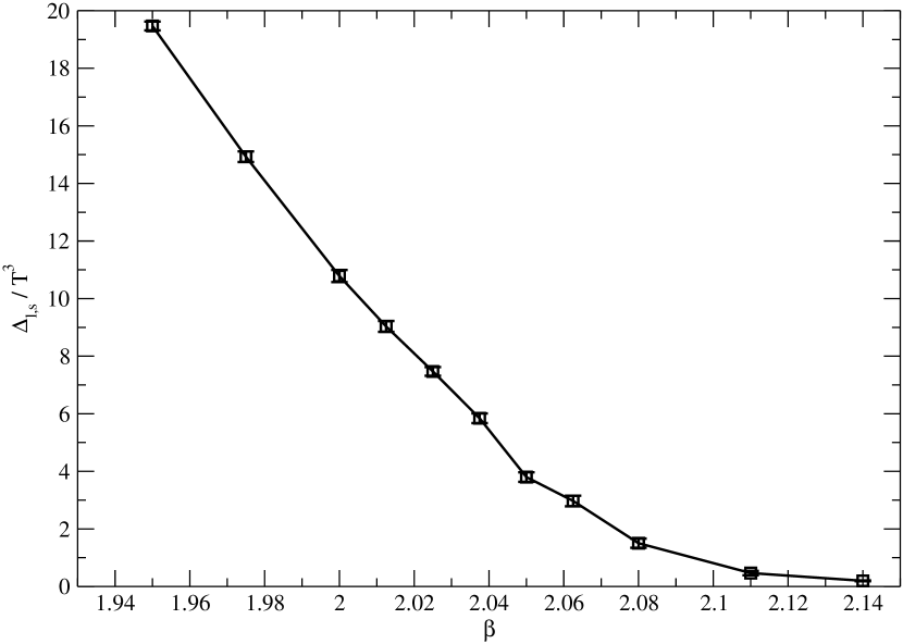
Figure 5: The subtracted light-quark chiral condensate, $\Delta_{l,s}=\langle\overline{\psi}_{l}\psi_{l}\rangle-m_{l}/m_{s}\langle\overline{\psi}_{s}\psi_{s}\rangle$ as a function of $\beta$. This subtraction removes the uninteresting $m_{l}/a^{2}$ contribution from $\langle\overline{\psi}_{l}\psi_{l}\rangle$, leaving a quantity which more accurately describes vacuum chiral symmetry breaking. This improvement is easily seen for the larger values of $\beta$, above the transition region, where this subtracted quantity vanishes, in contrast to the non-zero behavior seen for $\langle\overline{\psi}_{l}\psi_{l}\rangle$ in Fig. 2.

At finite quark mass the chiral condensate contains an unphysical, quadratically divergent, additive contribution coming from eigenvectors of the Dirac operator with eigenvalue $\lambda\sim 1/a$. These perturbative $\propto m_{f}/a^{2}$ terms will show no finite temperature effects and obscure the physically important contribution from vacuum chiral symmetry breaking. Since these terms enter both the light and strange condensates $\langle\overline{\psi}_{l}\psi_{l}\rangle$ and $\langle\overline{\psi}_{s}\psi_{s}\rangle$ in the same way it is appealing to remove this unphysical portion of $\langle\overline{\psi}_{l}\psi_{l}\rangle$ by subtracting $(m_{l}/m_{s})\langle\overline{\psi}_{s}\psi_{s}\rangle$ from it Cheng:2007jq . This should effectively remove the $m_{l}/a^{2}$ term from $\langle\overline{\psi}_{l}\psi_{l}\rangle$ while having little effect on the contribution from vacuum chiral symmetry breaking. The result for such a subtracted light chiral condensate is shown in Fig. 5.

The exact form for this subtraction is complicated for domain wall fermions by the presence of residual chiral symmetry breaking. In particular, the factor $m_{l}/m_{s}$ might be constructed from the bare input quark masses or from the more physical combination $(m_{l}+m_{\mathrm{res}})/(m_{s}+m_{\mathrm{res}})$. As is discussed in Section V.2, theoretical expectations and our numerical results suggest that the short-distance, $1/a^{2}$ portion of the chiral condensate will not show the $1/L_{s}$ behavior seen in the residual mass so this latter subtraction would not be appropriate. Instead, $\langle\overline{\psi}_{q}\psi_{q}\rangle$ approaches a constant rapidly with increasing $L_{s}$ and in the limit of infinite $L_{s}$ the ratio of the explicit chiral symmetry breaking parameters $m_{l}/m_{s}$ is the correct factor to use. Thus, it is this approach which is shown in Fig. 5.

III.2 Polyakov loop

For a pure $SU(3)$ gauge theory, there exists a first-order deconfining phase transition. The relevant order parameter in this case is the Polyakov loop, $L$, which is related to the free energy of an isolated, static quark, $V_{hq}$: $L\sim\exp(-V_{hq}/T)$. In the confined phase, producing an isolated quark requires infinite energy and the Polyakov loop vanishes. However, at sufficiently high temperatures, the system becomes deconfined and the Polyakov loop acquires a non-vanishing expectation value in a sufficiently large volume. The Polyakov loop and its susceptibility are defined in terms of lattice variables as:

$$L = \frac{1}{3N_{s}^{3}}\sum_{\vec{r}}\mathrm{Tr}\left(\prod_{t=0}^{N_{t}-1}U_{0}(\vec{r},t)\right)$$ (3)

$$\chi_{L} = N_{s}^{3}\left\{\langle L^{2}\rangle-\langle L\rangle^{2}\right\}.$$ (4)

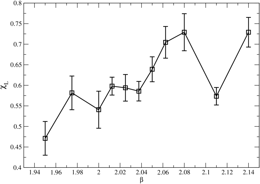
Figure 7: The Polyakov loop susceptibility plotted as a function of $\beta$.

Figures 6 and 7 show the Polyakov loop and the Polyakov loop susceptibility. As in the case of the chiral condensate, it is difficult to precisely locate an inflection point in the $\beta$ dependence of the Polyakov loop although the region where the Polyakov loop begins to increase more rapidly is roughly coincident with the peak in chiral susceptibility. There is no well-resolved peak in the data for the Polyakov loop susceptibility, so we are unable to use this observable to locate the crossover region. We list our results for these finite temperature quantities in Table 2.

$\beta$		$\langle\overline{\psi}_{l}\psi_{l}\rangle/T^{3}$	$\chi_{l}/T^{2}$	$\langle\overline{\psi}_{s}\psi_{s}\rangle/T^{3}$	$\chi_{s}/T^{2}$	$\langle L\rangle~{}(10^{-3})$	$\chi_{L}$
1.	95	22.8(2)	6.4(17)	40.9(1)	3.5(8)	4.40(62)	0.47(4)
1.	975	17.9(2)	8.2(14)	36.8(1)	4.1(7)	5.44(42)	0.58(4)
2.	00	13.5(2)	9.4(27)	33.2(1)	2.7(7)	6.52(47)	0.54(5)
2.	0125	11.6(2)	16.4(20)	31.6	5.7(7)	9.02(53)	0.60(2)
2.	025	9.9(2)	17.8(26)	30.2(1)	4.7(6)	10.18(61)	0.59(3)
2.	0375	8.2(2)	28.2(25)	28.9(1)	5.3(5)	13.61(55)	0.59(2)
2.	05	6.0(2)	20.5(18)	27.4(1)	4.5(8)	16.77(71)	0.64(3)
2.	0625	5.1(2)	20.7(27)	26.6(1)	4.2(5)	18.22(86)	0.70(4)
2.	08	3.5(2)	11.4(20)	25.2(1)	3.0(6)	25.91(129)	0.73(5)
2.	11	2.37(7)	3.7(30)	23.51(5)	0.9(2)	34.74(99)	0.57(2)
2.	14	2.03(2)	0.15(2)	22.59(7)	0.6(3)	45.6(20)	0.73(4)

Table 2: Results obtained for the light and strange quark chiral condensates and disconnected chiral susceptibilities as well as the Polyakov loop and its susceptibility.

III.3 Quark Number Susceptibilities

Calculations performed with staggered and Wilson fermions at finite temperature have shown that the analysis of thermal fluctuations of conserved charges, e.g. baryon number, strangeness or electric charge, gives sensitive information about the deconfining features of the QCD transition at high temperature. Charge fluctuations are small at low temperature, rapidly rise in the transition region and approach the ideal gas Stefan-Boltzmann limit at high temperature. These generic features are easy to understand. Charge fluctuations are small at low temperatures as charges are carried by rather heavy hadrons, while they are large at high temperature where the conserved charges are carried by almost massless quarks. Charge fluctuations therefore reflect deconfining aspects of the QCD transition.

Thermal fluctuations of conserved charges can be calculated from diagonal and off-diagonal quark number susceptibilities which are defined as second derivatives of the QCD partition function with respect to quark chemical potentials Gottlieb:1987ac , ($\mu_{u},\ \mu_{d},\ \mu_{s}$),

$$\frac{\chi_{2}^{f}}{T^{2}}=\frac{2c_{2}^{f}}{T^{2}} = \left.\frac{1}{VT^{3}}\frac{\partial^{2}\ln Z(V,T,\mu_{u},\mu_{d},\mu_{s})}{\partial(\mu_{f}/T)^{2}}\right|_{\mu_{f}=0}$$ (5)

$$= \frac{1}{VT^{3}}\left\{\Bigg{\langle}\text{tr}\left(M^{-1}_{f}\frac{\mathrm{d}^{2}M_{f}}{\mathrm{d}\mu^{2}_{f}}\right)\Bigg{\rangle}-\Bigg{\langle}\text{tr}\left(M^{-1}_{f}\frac{\mathrm{d}M_{f}}{\mathrm{d}\mu_{f}}M^{-1}_{f}\frac{\mathrm{d}M_{f}}{\mathrm{d}\mu_{f}}\right)\Bigg{\rangle}\right.$$

$$\;\;\;\;\;\;\;\;\;\left.+\Bigg{\langle}\text{tr}^{2}\left(M^{-1}_{f}\frac{\mathrm{d}M_{f}}{\mathrm{d}\mu_{f}}\right)\Bigg{\rangle}\right\}\;\;,\;\;f=u,\ d,\ s\ ,$$

$$\frac{\chi_{11}^{fg}}{T^{2}}=\frac{c_{11}^{fg}}{T^{2}} = \left.\frac{1}{VT^{3}}\frac{\partial^{2}\ln Z(V,T,\mu_{u},\mu_{d},\mu_{s})}{\partial\mu_{f}/T\ \partial\mu_{g}/T}\right|_{\mu_{g}=\mu_{f}=0}$$ (6)

$$= \frac{1}{VT^{3}}\Bigg{\langle}\text{tr}\left(M^{-1}_{f}\frac{\mathrm{d}M_{f}}{\mathrm{d}\mu_{f}}\right)\text{tr}\left(M^{-1}_{g}\frac{\mathrm{d}M_{g}}{\mathrm{d}\mu_{g}}\right)\Bigg{\rangle}\;\;,\;\;f,g=u,\ d,\ s\ ,\ f\neq g\ ,$$

where $c_{2}^{f}$ and $c_{11}^{fg}$ are the second-order coefficients in a Taylor expansion of $p/T^{4}$.

In the DWF formalism the introduction of quark chemical potentials is straightforward Bloch:2007xi ; Hegde:2008nx ; Gavai:2008ea . It follows the same approach used in other fermion discretization schemes Hasenfratz:1983ba , i.e. in the fermion determinant for quarks of flavor $f$ the parallel transporters in forward [backward] time direction are multiplied with exponential factors $\exp(\mu_{f}a)$ [$\exp(-\mu_{f}a)$], respectively . Since these time direction parallel transporters couple to the fermion fields for all locations $0\leq s<L_{s}$ in the fifth dimension, fermionic charge is assigned in a consistent way throughout the fifth dimension. Just as in the case of the fermionic action Furman:1994ky ; Vranas:1997da , a precaution must be taken to ensure that unphysical, 5-dimensional modes do not begin to contribute as $L_{s}$ becomes large. The contribution of individual 5-dimension modes, not bound to the $s=0$ or $s=L_{s}-1$ walls, will vanish in the continuum limit. However, for finite lattice spacing and large $L_{s}$ the number of these modes may be sufficient to distort physical quantities. In our calculation this is avoided by adding an additional compensating Pauli-Villars pseudo-fermion field for each quark flavor. Thus, the chemical potential $\mu_{f}$ for each quark flavor enters the time parallel transporters for both the light quark and the corresponding Pauli-Villars pseudo-fermion carrying that flavor. These Pauli-Villars fields have $m_{f}=1$ and therefore satisfy anti-periodic boundary conditions in the 5-dimension. Thus, they contribute no “physical” 4-dimensional surface states but act to cancel any possible bulk contributions $\propto L_{s}$ introduced by the domain wall quarks.

Introducing chemical potentials for conserved charges, e.g. baryon number ($\mu_{B}$), strangeness ($\mu_{S}$) and electric charge ($\mu_{Q}$), allows us to define susceptibilities (charge fluctuations) by taking derivatives with respect to these chemical potentials ,

$$\frac{\chi_{2}^{X}}{T^{2}}=\frac{2c_{2}^{X}}{T^{2}} = \frac{1}{VT^{3}}\frac{\partial^{2}\ln Z(V,T,\mu_{B},\mu_{S},\mu_{Q})}{\partial(\mu_{X}/T)^{2}}|_{\mu_{X}=0}\;\;,\;\;X=B,\ S,\ Q$$ (7)

Expressed in terms of quark number susceptibilities, one finds,

$$c_{2}^{S} = c_{2}^{s}$$ (8)

$$c_{2}^{B} = \frac{1}{9}\left(2c^{u}_{2}+c^{s}_{2}+c^{ud}_{11}+2c^{us}_{11}\right)$$ (9)

$$c_{2}^{Q} = \frac{1}{9}\left(5c^{u}_{2}+c^{s}_{2}-2c^{ud}_{11}-c^{us}_{11}\right)$$ (10)

Similar to the chiral susceptibility, the two derivatives appearing in Eq. 5 generate ’disconnected’ and ’connected’ contributions to the flavor diagonal susceptibilities. The mixed susceptibilities defined in Eq. 6, on the other hand, only receive contributions from disconnected terms. As the disconnected terms are much more noisy than the connected terms, those susceptibilities that are dominated by contributions from the latter are generally easier to calculate. This makes the electric charge susceptibility and the isospin susceptibility, $\displaystyle{c_{2}^{I}=\left(2c^{u}_{2}-c^{ud}_{11}\right)/4}$, most suitable for our current, exploratory analysis with domain wall fermions.

$\beta$	measurements	separation	random vectors	$c_{2}^{u}$	$c_{2}^{s}$	$c_{2}^{I}$	$c_{2}^{Q}$
1.95	73	10	200	0.08(11)	0.01(5)	0.046(8)	0.060(10)
1.975	61	10	200	0.03(10)	0.03(7)	0.070(8)	0.085(10)
2.0125	125	10	150	0.22(6)	0.16(2)	0.119(7)	0.148(10)
2.025	71	20	150	0.30(5)	0.19(3)	0.141(6)	0.176(8)
2.0375	96	20	150	0.30(6)	0.16(2)	0.160(6)	0.205(8)
2.05	81	25	150	0.38(5)	0.25(4)	0.191(9)	0.243(11)
2.0625	111	10	150	0.32(6)	0.24(4)	0.200(9)	0.252(10)
2.11	35	10	100	0.51(6)	0.44(5)	0.233(11)	0.303(14)
2.14	40	10	100	0.51(3)	0.43(2)	0.256(4)	0.333(5)

Table 3: Details of the calculation of quark number susceptibilities. The column labeled ”measurements” gives the number of measurements that were performed. That labeled ”separation” gives the number of time units between those measurements while the ”random vectors” column gives the number of random vectors used in each measurement.

Computing the susceptibilities involves measuring traces of operators. We used stochastic estimators with 100-200 random vectors per configuration. Our measurements are summarized in Table 3. Some of the results presented here have been shown previously Hegde:2008rm .

In Fig. 8, we show our results for the diagonal, light and strange quark number, susceptibilities $c_{2}^{u}$ and $c_{2}^{s}$, respectively. We see that these susceptibilities do transit from a low value to a high one as $\beta$ increases. However, given the current statistical accuracy of our calculation, it is difficult to assign any definite value of $\beta$ around which the transition takes place. To a large extent the fluctuations observed in the data arise from contributions of off-diagonal susceptibilities, $c_{11}^{fg}$, with $f\equiv g$. In fact, with our current limited statistics these susceptibilities vanish within errors and therefore only contribute noise to the diagonal susceptibilities.

The disconnected parts however, either completely or partially cancel out in the two susceptibilities $c_{2}^{I}$ and $c_{2}^{Q}$. As a result, one obtains much better results for these quantities, as seen in Fig. 9.

We have tried to determine the inflection point for the electric charge and isospin susceptibilities, which may serve as an estimate for the transition point, although the slope of these observables also receives contributions from the regular part of the free energy. We have fit the data using two different fit ansätze,

$$f_{I}(\beta) = A\tanh(B(\beta-\beta_{0}))+C\;,$$

$$f_{II}(\beta) = A_{3}+B_{3}\beta+C_{3}\beta^{2}+D_{3}\beta^{3}\;.$$ (11)

To estimate systematic errors in the fits we performed fits for the entire data set as well as in limited ranges by leaving out one or two data points at the lower as well as upper edge of the $\beta$-range covered by our data sample. From this we find inflection points in the range $2.024\leq\beta_{0}\leq 2.037$ for $c_{2}^{I}$ and $2.024\leq\beta_{0}\leq 2.034$ for $c_{2}^{Q}$. Summarizing this analysis we therefore conclude that the inflection points in the electric charge and isospin susceptibilities coincide within statistical errors and are given by $\beta_{0}=2.030(7)$. This is in good agreement with the determination of a pseudo-critical coupling obtained from the location of peak in the chiral susceptibility, $\beta=2.0375$, found in Section III.1.

IV Zero temperature observables

In this section we present the results for physical quantities at zero temperature computed on a $16^{3}\times 32$ lattice for $\beta=2.025$ which, as Fig. 3 suggests, lies in the lower temperature part of the $N_{t}=8$ transition region.

IV.1 Static quark potential

To determine the lattice scale, we measured the static quark-anti-quark correlation function, $W(r,t)$, on 148 configurations (every 5 MD trajectories from 300-1035) on these zero temperature configurations. The quantity $W(r,t)$ is the product of two spatially separated sequences of temporal gauge links connecting spatial hyperplanes, each containing links that have been fixed to Coulomb gauge Bernard:2000gd ; Li:2006gra :

$$W(r,t) = \frac{1}{N_{\mathrm{pairs}}(r)}\sum_{\left|\vec{r}_{1}-\vec{r}_{2}\right|=r}\mbox{tr}\Bigl{\{}U_{0}(\vec{r}_{1},0)U_{0}(\vec{r}_{1},1)\dots U_{0}(\vec{r}_{1},t-1)$$

$$\hskip 108.405pt\cdot U_{0}^{\dagger}(\vec{r}_{2},t-1)\dots U_{0}^{\dagger}(\vec{r}_{2},1)U_{0}^{\dagger}(\vec{r}_{2},0)\Bigr{\}},$$

where $N_{\mathrm{pairs}}(r)$ is the number of pairs of lattice points with a given spatial separation $r$. In our calculation the results obtained from orienting the “time” axis along each of the four possible directions are also averaged together. The time dependence of $W(r,t)$ was then fit to an exponential form in order to extract the static quark potential $V(r)$:

$$W(r,t)=c(r)\exp\left(-V(r)t\right).$$ (13)

The potential $V(r)$ was subsequently fit to the Cornell form, and used to determine the Sommer parameter $r_{0}$, as defined below:

$$V(r) = -\frac{\alpha}{r}+\sigma r+V_{0}$$ (14)

$$\left(r^{2}\frac{dV(r)}{dr}\right)_{r=r_{0}} = 1.65\;.$$ (15)

Table 4 gives the details of the fit which determines the parameters $\alpha$ and $\sigma$ of Eq. 14 and results in a value of $r_{0}/a=3.08(9)$. For the physical value of $r_{0}$, we use the current standard result $r_{0}=0.469(7)$ fm Gray:2005ur . This gives a lattice spacing $a\approx 0.15$ fm, or $a^{-1}\approx 1.3$ GeV. It should be emphasized that this value for $r_{0}$ has been determined for a single light quark mass and no extrapolation to the physical value of the light quark mass has been performed. This failure to extrapolate to a physical value for the light quark mass is likely to result in an overestimate of the lattice spacing $a$ by about 3%.

$\beta$	$r_{0}/a$	$a^{-1}$ (GeV)	t fit range	r fit range	$\chi^{2}/$dof.
2.025	3.08(9)	1.30(4)	$(4,9)$	$(\sqrt{3},6)$	1.03

Table 4: Results for $r_{0}$. The errors are calculated by the jackknife method, with data binned into blocks, each containing 10 molecular dynamics time units.

IV.2 Meson mass spectrum

In addition to the static quark potential, we also calculated the meson spectrum on the same zero temperature ensemble at $\beta=2.025$. The meson spectrum was determined using 55 configurations, separated by 10 MD time units, from 500 and 1040. Table 5 gives the results for $m_{\rho}$ and $m_{\pi}$ for three different valence mass combinations, as well as their values in the chiral limit from linear extrapolation. Equating the physical value of $m_{\rho}=776$ MeV with the chirally extrapolated lattice value gives a lattice scale of $a^{-1}=1.26(11)$ GeV, which is consistent with the scale determined from $r_{0}$. Examining the data for the light pseudoscalar meson, we find $m_{\pi}\approx 308$ MeV, somewhat larger than twice the mass of the physical pion. For the kaon, we have $m_{K}\approx 496$ MeV, very close to the physical kaon mass.

$m_{x}^{val}$	$m_{y}^{val}$	$m_{\mathrm{avg}}$	fit range	$m_{\rho}a$	$\chi^{2}$/dof	$m_{\pi}a$	$\chi^{2}$/dof
0.003	0.003	0.0030	8-16	0.646(63)	0.3(4)	0.2373(20)	2.4(11)
0.003	0.037	0.0200	8-16	0.716(23)	0.8(7)	0.3815(15)	2.0(10)
0.037	0.037	0.0370	8-16	0.776(10)	2.2(11)	0.4846(11)	1.2(8)
	$-m_{\mathrm{res}}$			0.617(56)		0.073(6)

Table 5: The calculated masses $m_{\rho}$ and $m_{\pi}$ for various combinations of valence quark mass. The last line represents extrapolation of the light quark mass to $m_{\mathrm{avg}}=(m_{x}+m_{y})/2=-m_{\mathrm{res}}$.

V Residual Chiral Symmetry breaking

We now examine the central question in such a coarse-lattice calculation using domain wall fermions: the size and character of the residual chiral symmetry breaking effects. We examine the residual mass computed at finite temperature, its $L_{s}$ dependence and the dependence of the chiral condensate on $L_{s}$. In both cases we examine the value of $L_{s}=32$ used for the dynamical quarks as well as ”non-unitary”, valence values of $L_{s}$ varying between 8 and 128.

V.1 Residual Mass

One of the primary difficulties with the calculation presented here is the rather large residual chiral symmetry breaking at the parameters that we employ. This manifests itself in a value for the residual mass, $m_{\mathrm{res}}$ which is larger than the input light quark mass, $m_{ud}=0.003$ over almost the entire temperature range of our calculation.

For the Iwasaki gauge action, the residual chiral symmetry breaking has been extensively studied by the RBC-UKQCD collaboration for $\beta\geq 2.13$ and $L_{s}=16$ Antonio:2006px ; Allton:2007hx ; Antonio:2008zz ; Allton:2008pn . However, the lattice ensembles that we use here are significantly coarser, resulting in larger residual chiral symmetry breaking, even for our increased value of $L_{s}=32$.

$\beta$	$m_{\mathrm{res}}$ ($m_{f}=0.003$)	$m_{\mathrm{res}}$ ($m_{f}=0.037$)
1.95	0.0253(5)	0.0244(5)
2.00	0.0105(3)	0.0095(2)
2.025	0.0069(3)	0.0059(3)
2.05	0.0046(5)	0.0034(2)
2.08	0.0023(5)	0.0016(2)
2.11	0.0011(2)	0.0009(1)
2.14	0.0010(4)	0.0006(2)

Table 6: The residual mass as a function of $\beta$ computed on the finite temperature, $16^{3}\times 8$ lattice volume.

$m_{\textrm{val}}$	$m_{\rm res}$	fit range
0.003	0.006647(84)	8-16
0.020	0.006227(74)	8-16
0.037	0.005835(71)	8-16
0.000	0.006713(85)

Table 7: The residual mass as a function of valence quark mass computed on the zero temperature, $16^{3}\times 32$ lattice volume with $\beta=2.025$, with the extrapolated $m_{\textrm{val}}\rightarrow 0$ value.

$L_{s}$	$m_{\mathrm{res}}$ ($m_{f}=0.003$)	$m_{\mathrm{res}}$ ($m_{f}=0.037$)
8	0.0529(9)	0.0508(7)
16	0.0235(5)	0.0220(4)
32	0.0105(3)	0.0095(2)
64	0.0048(3)	0.0044(3)
128	0.0024(2)	0.0025(2)

Table 8: The residual mass as a function of the valence $L_{s}$ computed on a $16^{3}\times 8$ lattice volume with $\beta=2.00$.

Table 6 shows our results for $m_{\mathrm{res}}$ on several of the $16^{3}\times 8$ finite temperature ensembles. We follow the standard method, described for example in Ref. Antonio:2006px , determining the residual mass by computing the ratio of the midpoint correlator to the pion correlator evaluated at source-sink separations sufficiently large to suppress short-distance lattice artifacts. This is most easily done on these finite temperature lattices by choosing the source-sink separation to lie in a spatial rather than temporal direction.

Table 7 gives $m_{\mathrm{res}}$ on the $16^{3}\times 32$ ensemble at $\beta=2.025$ where the correlators are measured in the temporal direction. It is important to observe that the values of $m_{\mathrm{res}}$ determined at $\beta=2.025$ at finite and zero temperature, 0.0069(5) and 0.006647(84) respectively, are consistent. This is an important check on the domain wall method since $m_{\mathrm{res}}$ should be a temperature-independent constant representing the leading long-distance effects of residual chiral symmetry breaking.

Table 8 shows results for $m_{\mathrm{res}}$ evaluated at different values for the valence $L_{s}$ at $\beta=2.00$. The expected behavior of $m_{\mathrm{res}}$ as a function of $L_{s}$ is given by Antonio:2008zz :

$$m_{\mathrm{res}}(L_{s})=\frac{c_{1}}{L_{s}}\exp(-\lambda_{c}L_{s})+\frac{c_{2}}{L_{s}}.$$ (16)

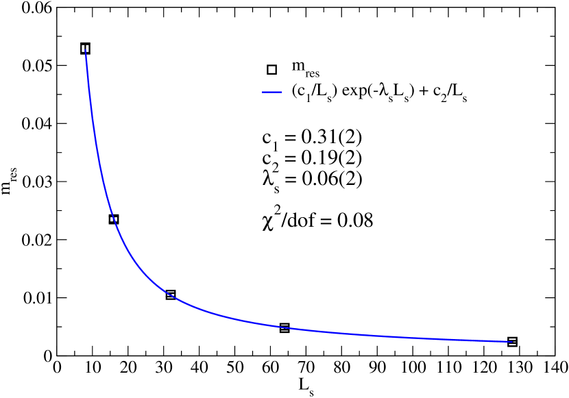
Figure 10: The residual mass $m_{\mathrm{res}}$ is plotted versus $L_{s}$ for $\beta=2.00$, $16^{3}\times 8$. The fit to Eq. 16 is also shown.

Here the exponential term comes from extended states with eigenvalues near the mobility edge, $\lambda_{c}$, while the $1/L_{s}$ piece reflects the presence of localized modes with small eigenvalues and is proportional to the density of such small eigenvalues at $\lambda=0$ Golterman:2003qe ; Golterman:2004cy ; Golterman:2005fe ; Antonio:2008zz . This formula describes our data very well as can be seen from Fig. 10 where both the data presented in Table 7 and the resulting fit to Eq. 16 are shown. The proportionality of $m_{\mathrm{res}}$ to $1/L_{s}$ shown in Table 8 for $L_{s}\geq 32$ indicates that our choice of $L_{s}=32$ has effectively suppressed the exponential term in Eq. 16 but that a large contribution remains from the significant density of near-zero eigenvalues on our relatively coarse lattice.

Since we have chosen the input light quark mass $m_{l}=0.003$ to be fixed for the different values of $\beta$, the strong dependence of $m_{\mathrm{res}}$ on $\beta$ shown in Table 6 means that the total light quark mass, $m_{q}=m_{l}+m_{\mathrm{res}}$, changes significantly in the crossover region, from $m_{q}\approx 0.0075$ at $\beta=2.05$ increasing to $m_{q}\approx 0.013$ at $\beta=2.00$. This substantial increase may significantly affect the quantities whose temperature dependence we are trying to determine.

V.2 Chiral condensate and susceptibility at varying $L_{s}$

The change in the total quark mass as we vary $\beta$ is expected to cause a distortion of the chiral susceptibility curve that we use to locate the crossover transition. In order to understand how this varying mass affects our results, we have computed the chiral condensate and its susceptibility with different choices for the valence $L_{s}$ and valence $m_{l}$ at several values of $\beta$.

In one set of measurements, we increased $L_{s}$ from 32 to 64, while keeping the input quark masses fixed at $m_{l}=0.003$ and $m_{s}=0.037$. This has the result of reducing the total light and strange quark masses, as the residual masses are reduced by approximately a factor of two. In another set of measurements, we increased $L_{s}$ to 96 but adjusted the input quark masses to compensate for the reduced residual mass so that the total light and strange quark masses, $m_{l}+m_{res}$ and $m_{s}+m_{res}$ respectively, matched those in the $L_{s}=32$ calculation for each value of beta. Finally, for one value of the gauge coupling, $\beta=2.0375$, we used several choices of valence $L_{s}$ (8, 16, 24, 48) at fixed input quark mass $(m_{l},m_{s})=(0.003,0.037)$ in order to examine the $L_{s}$ dependence of our observables at fixed $\beta.$ Table 9 gives the results of these measurements. Figures 2 and 3 show the results with the valence $L_{s}=64$ and $L_{s}=96$ in context with the $L_{s}=32$ results.

$L_{s}$	$\beta$	$m_{l}$	$\langle\overline{\psi}_{l}\psi_{l}\rangle/T^{3}$	$\chi_{l}/T^{2}$	$m_{s}$	$\langle\overline{\psi}_{s}\psi_{s}\rangle/T^{3}$	$\chi_{s}/T^{2}$
8	2.0375	0.003	26.6(1)	7.2(8)	0.037	45.5(1)	4.3(5)
16			10.8(1)	12.4(1)		31.1(1)	4.4(5)
24			8.6(1)	17.8(2)		29.4(1)	4.6(6)
48			7.8(2)	33.2(5)		28.5(1)	5.0(8)
64	2.0125	0.003	11.2(2)	32.3(3)	0.037	31.0(1)	6.5(6)
	2.025		9.7(1)	32.6(4)		29.7(1)	5.1(8)
	2.0375		8.0(2)	46.2(8)		28.4(1)	4.9(7)
	2.05		5.9(2)	39.0(4)		27.1(1)	5.3(7)
96	2.00	0.0078	17.0(4)	13.6(36)	0.0418	36.4(2)	1.9(11)
	2.0375	0.0063	9.8(1)	24.8(26)	0.0403	30.4(1)	4.9(6)
	2.05	0.0070	8.4(1)	20.2(23)	0.0410	29.4(1)	4.1(6)

Table 9: Results for $\langle\overline{\psi}_{q}\psi_{q}\rangle$ and the corresponding disconnected susceptibility in which some of the values for $L_{s}$ and $m_{l}$, assigned to the quark loop present in the $\overline{\psi}_{q}\psi_{q}$ observable, differ from those that appear in the quark determinant.

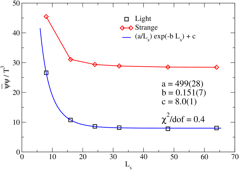
Figure 11: Chiral condensate versus the valence $L_{s}$ for $\beta=2.0375$, on a $16^{3}\times 8$ lattice volume. The fit to Eq. 17 for $\overline{\psi}_{l}\psi_{l}/T^{3}$ is also shown.

From Fig. 2, we see that increasing $L_{s}$ from 32 to 64 while keeping the input quark masses fixed does not have much effect on the chiral condensate for each $\beta$ at which we measure. On the other hand, using $L_{s}=96$ and larger input quark masses causes a noticeable increase in the chiral condensate. A closely related phenomenon can be found in Fig. 11 which shows the dependence of $\langle\overline{\psi}_{q}\psi_{q}\rangle$ on $L_{s}$ at the single value of $\beta=2.0375$. For small values of $L_{s}$, there is a strong $L_{s}$ dependence, but the chiral condensate quickly plateaus to an approximately constant value for $L_{s}>32$, even though $m_{\mathrm{res}}$ and thus the total light quark mass is still changing significantly as $L_{s}$ increases above 32.

This contrast between the $L_{s}$ dependence of $\langle\overline{\psi}_{q}\psi_{q}\rangle$ and $m_{\rm res}$ can be made more precise if we attempt to fit the $L_{s}$ dependence of $\langle\overline{\psi}_{q}\psi_{q}\rangle$ by a single exponential, omitting the power law piece that is important in $m_{\rm res}(L_{s})$:

$$\langle\overline{\psi}_{q}\psi_{q}\rangle(L_{s})=\frac{a}{L_{s}}~{}\exp(-bL_{s})+c.$$ (17)

This fit describes the data very well, giving $\chi^{2}$/dof = 0.4, in strong contrast to $m_{\rm res}(L_{s})$ where the $c_{2}/L_{s}$ term in Eq. 16 is required to fit the data. Thus, it appears that the contribution of the localized modes, responsible for the $c_{2}/L_{s}$ term in Eq. 16, is much less important for the chiral condensate than for the residual mass.

In fact, this is to be expected. The localized states are rather special. They are associated with the near zero modes of the 4-D Wilson Dirac operator evaluated at a mass equal to the domain wall height, $-M_{5}$. They are non-perturbative and appear when topology changes. They are thus related to continuum physics and are limited in number. In contrast, the extended states which give the exponential term $\exp(-\lambda_{c}L_{s})/L_{s}$ can be seen in perturbation theory, correspond to large, $O(1/a)$ eigenvalues of $D_{W}^{4D}(-M_{5})$ and are far more numerous with a density given by four-dimensional free-field phase space at the $\lambda\sim 1/a$ scale. Since the perturbative contribution to the dimension-one residual mass behaves as $1/a$ while that to the dimension-three chiral condensate as $1/a^{3}$, it is to be expected that the non-perturbative, localized states will play a much larger role in the former.

If we accept that the $L_{s}$ behavior of the chiral condensate differs in this way from that of the residual mass, then the behavior of the chiral condensate shown in Fig. 2 becomes easy to understand. In contrast to the total quark mass $m_{f}+m_{\rm res}$ which depends significantly on both the input bare mass $m_{f}$ and on $L_{s}$ through $m_{\rm res}$, the chiral condensate is expected to depend only on the input bare mass $m_{f}$. In fact this dependence is quite strong with the familiar form $m_{f}/a^{2}$. Thus, when we keep $m_{f}$ fixed and simply increase $L_{s}$ from 32 to 64 we should expect little change in $\langle\overline{\psi}_{q}\psi_{q}\rangle$ as is shown in Fig. 2. However, for the second set of points where $L_{s}$ is increased to 96 and $m_{f}$ is also increased to keep $m_{f}=m_{\rm res}$ fixed, the increase in the bare input quark mass $m_{f}$ produces a significant increase in $\langle\overline{\psi}_{q}\psi_{q}\rangle$.

As will become clear below, the above discussion of the chiral condensate is approximate, focusing on the dominant explicit chiral symmetry breaking term $m_{f}/a^{2}$ coming from the input quark mass and a residual chiral symmetry breaking piece expected to behave as $\exp(-\lambda_{c}L_{s})/a^{3}$. The more interesting, physical contribution to the chiral condensate which arises from vacuum symmetry breaking and is described, for example, by the Banks-Casher formula, will depend on the physical quark mass, $m_{f}+m_{\mathrm{res}}$. Such dependence on $m_{\mathrm{res}}$ will necessarily introduce a $1/L_{s}$ dependence on $L_{s}$, not seen in the results described in the paragraph above. This is to be expected because the much larger $m_{f}/a^{2}$ and $\exp(-\lambda_{c}L_{s})/a^{3}$ terms do not show this behavior.

In contrast to the chiral condensate, the disconnected part of the chiral susceptibility is more physical and grows with decreasing quark mass. It is dominated by the large fluctuations present in the long-distance modes. The large $m_{f}/a^{2}$ and $\exp(-\lambda_{c}L_{s})/a^{3}$ which dominate the averaged $\langle\overline{\psi}_{q}\psi_{q}\rangle$ fluctuate less because of the large number of short distance modes and hence contribute relatively little to the fluctuations in the quantity $\overline{\psi}_{q}\psi_{q}$. This behavior should be contrasted to that of the connected chiral susceptibility which is again dominated by short-distance modes and hence of less interest and not considered here.

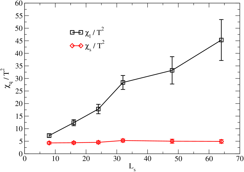
Figure 12: Disconnected chiral susceptibility versus $L_{s}$ for $\beta=2.0375$, $16^{3}\times 8$, with input quark masses fixed to $m_{l}=0.003$ and $m_{s}=0.037$.

Thus, for small quark mass and $\beta\approx\beta_{c}$ we expect that the disconnected chiral susceptibility will depend on the total effective quark mass, $m_{q}=m_{l}+m_{\mathrm{res}}$, that enters into the low energy QCD Lagrangian. Figure 12 shows the disconnected chiral susceptibility at $\beta=2.0375$ as a function of the valence $L_{s}$. The chiral susceptibility does not plateau as $L_{s}$ grows. Rather, it increases as the total quark mass $m_{q}=m_{l}+m_{\mathrm{res}}$ is decreased as we move to larger $L_{s}$. The fact that the chiral susceptibility depends only on the total quark mass can also be seen in the measurements at $L_{s}=96$, where the input quark masses are adjusted to keep the total quark mass fixed. As we can see in Fig. 3, the chiral susceptibility at $L_{s}=96$ is roughly the same as at $L_{s}=32$, even though the relative sizes of the input quark masses and the residual mass has changed dramatically. This behavior provides a reassuring consistency check on the DWF approach: even at finite temperature the light fermion modes carry the expected quark mass, $m_{q}=m_{l}+m_{\mathrm{res}}$.

VI Locating $T_{c}$

We will now attempt to combine our finite and zero temperature results to determine the pseudo-critical temperature, $T_{c}$. As discussed in Section III and shown in Fig. 3, the chiral susceptibility shows a clear peak whose location gives a value for $\beta_{c}$. The result for $\beta_{c}$ is consistent with the region of rapid increase in the Polyakov loop and quark number susceptibilities seen in Figs. 6 and 9. Even though $\beta_{c}$ is fairly well resolved, there are still significant uncertainties in extracting a physical value of $T_{c}$ from our calculation. The most important issues are:

• The distortion in the dependence of the chiral susceptibility on $\beta$ induced by the variation of $m_{\mathrm{res}}$ with $\beta$.

• The uncertainty in determining the lattice scale at the peak location near $\beta_{c}=2.0375$ from our calculation of $r_{0}/a$ at $\beta=2.025$, performed with light quarks considerably more massive than that those found in nature.

• The absence of chiral and continuum extrapolations.

We address each of these sources of uncertainty in turn.

VI.1 Correcting for $m_{\mathrm{res}}(\beta)$

In Section III, we observed that the chiral susceptibility has a peak near $\beta=2.0375$, which we can identify as the center of the transition region. However, the total light quark mass $m_{q}=m_{l}+m_{\mathrm{res}}$ is different for each value of $\beta$ because of the changing residual mass $m_{\mathrm{res}}(\beta)$. This changing quark mass distorts the shape of the chiral susceptibility curve, shifting the location of its peak from what would be seen were we to have held the quark mass $m_{q}=m_{l}+m_{\mathrm{res}}$ fixed as $\beta$ was varied.

	Gaussian		Lorentz
$\alpha$	$\beta_{c}$	$\chi^{2}$/dof	$\beta_{c}$	$\chi^{2}$/dof
0	2.041(2)	1.7	2.041(2)	2.3
1/2	2.036(3)	1.7	2.035(3)	1.7
1	2.030(3)	1.7	2.030(3)	1.8
3/2	2.024(5)	1.8	2.026(3)	2.0

Table 10: The corrected peak location ($\beta_{c}$) in the light chiral susceptibility determined from fits to Lorentzian and Gaussian peak shapes resulting from different assumptions for the light quark mass dependence of $\chi_{l}$: $\chi_{l}/T^{2}\sim 1/(m_{l}+m_{res})^{\alpha}$). All fits include the 7 data points nearest the peak location, i.e. $\beta\in[2.00,2.08]$.

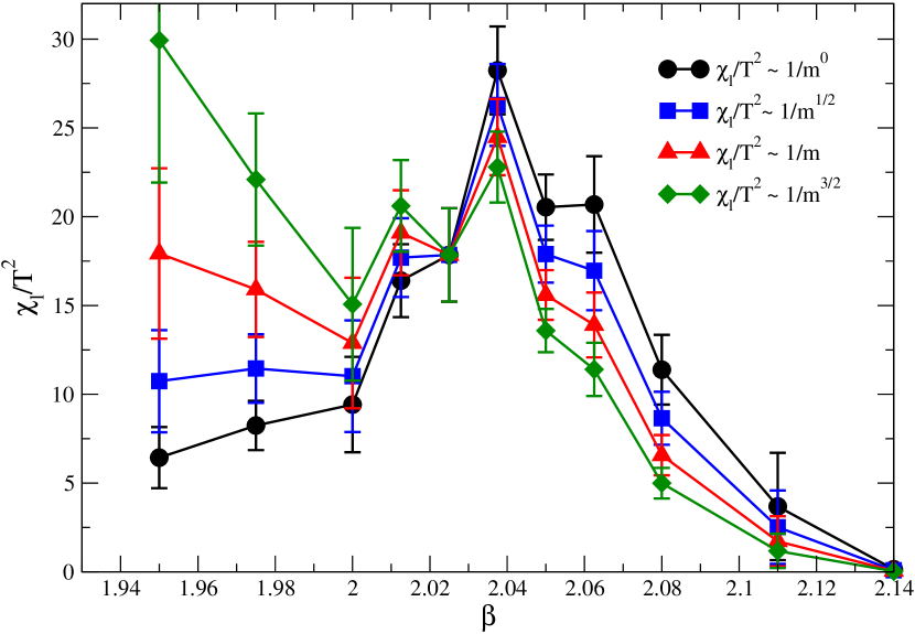
Figure 13: Light quark chiral susceptibility, where different assumptions for mass dependence are used to adjust the data to a constant bare light quark mass $(m_{l}+m_{\mathrm{res}})a=0.0097$, corresponding to the value at $\beta=2.025$, $L_{s}=32$ in our simulations.

In order to correct for this effect, we must account for the quark mass dependence of the chiral susceptibility. Our valence measurements at $L_{s}=64$ and $L_{s}=96$ indicate that the chiral susceptibility is inversely related to the quark mass and depends only on the combination $m_{q}=m_{l}+m_{\mathrm{res}}$. Figure 13 shows the resulting chiral susceptibility, when one corrects for the known $\beta$ dependence of $m_{\mathrm{res}}(\beta)$ by assuming a power-law dependence of $\chi_{l}\propto 1/m_{q}^{\alpha}$ on the quark mass for various choices of the power $\alpha$ ranging between $\alpha=0$ and $\alpha=3/2$.

While for $T\leq T_{c}$ and in the limit of small quark mass the chiral susceptibility is expected to behave as $\propto 1/\sqrt{m_{q}}$ Gasser:1986vb ; Hasenfratz:1989pk ; Smilga:1993in ; Smilga:1995qf ; Ejiri:2009ac corresponding to $\alpha=1/2$, our data from the $L_{s}=64$ valence measurements suggest $\alpha\sim 1.2-1.8$, albeit with rather large uncertainty. While $\alpha>0.5$ is inconsistent with the expected chiral behavior, we conservatively include such larger exponents as a possible behavior over our limited range of non-zero quark mass. Adjusting the chiral susceptibility curve in this manner enhances the chiral susceptibility at stronger coupling, as $m_{\mathrm{res}}(\beta)$ is larger on the coarser lattices. This causes a systematic shift in the peak location to stronger coupling when this correction is made.

While a cursory examination of Fig. 13 suggests that this correction does not change the peak structure, more careful study reveals that for the extreme $\alpha=1.5$ case the peak may have disappeared if the two lowest $\beta$ values with large errors are taken seriously. We view this possibility as unlikely but not absolutely ruled out.

Table 10 gives the results of fitting the peak region to Lorentzian and Gaussian peak shapes for various $\alpha.$ If we make no adjustment to the raw data ($\alpha=0$), we obtain $\beta_{c}=2.041(2)$. However, with $\alpha=3/2$, we have $\beta_{c}=2.024(5)$ with the Gaussian fit. While $\alpha=3/2$ seems to be favored by our valence measurements, we would like to emphasize that the quark mass dependence of the chiral susceptibility has large uncertainties. In particular, since we performed valence measurements at only three values of $\beta$, it is unclear if this $\alpha\approx 3/2$ behavior holds over a broader range in $\beta$. Also, we do not know whether the same mass dependence will persist if both the valence and dynamical quark masses are varied.

It should be recognized that if $\chi_{l}\propto 1/m_{q}^{\alpha}$ behavior for $T\leq T_{c}$ persists in the limit of vanishing $m_{q}$ the peak structure suggested by Fig. 13 may take on the appearance of a shoulder as the $\chi_{l}$ grows for $T<T_{c}$. Such a singular behavior at small quark mass, for example the $\alpha=1/2$ case suggested by chiral symmetry, would make $\chi_{l}$ a poor observable to locate the finite temperature transition Karsch:2008ch . Although our data shows an easily identified peak, unclouded by a large $1/\sqrt{m_{q}}$ term for $T\leq T_{c}$, it is possible that such behavior may substantially distort the chiral susceptibility as the light quark mass is decreased from that studied here to its physical value.

With these caveats in mind, we estimate the pseudo-critical coupling to be $\beta_{c}=2.03(1)$. The central value corresponds to the peak location if we assume a quark mass dependence of $\chi_{l}\sim 1/(m_{q}+m_{\mathrm{res}})$. The quoted error reflects the uncertainty in the mass dependence of $\chi_{l}$, and is chosen to encompass the range of values for $\beta_{c}$ shown in Table 10.

VI.2 Extracting the lattice scale at $\beta_{c}$

This value of $\beta_{c}$ differs from that of our zero-temperature ensemble ($\beta=2.025$) where we have measured the Sommer parameter, $r_{0}/a$. Thus, in order to determine the lattice scale at $\beta_{c}$, we need to know the dependence of $r_{0}/a$ on $\beta$. Fortunately, in addition to our measurements at $\beta=2.025$, $r_{0}/a$ has been extensively measured at $\beta=2.13$ Li:2006gra .

At $\beta=2.13$, the value of $r_{0}/a$ at the quark mass corresponding most closely to the current calculation is $r_{0}/a=3.997(22)$. Extrapolation to the chiral limit gives $r_{0}/a=4.113(31)$ for $\beta=2.13$, an approximately $3\%$ increase. A study of finite volume effects in Ref. Li:2006gra suggests that, in addition, the value computed on a $16^{3}\times 32$ lattice is too low by approximately $1-2\%$.

To obtain $r_{0}/a$ at $\beta_{c}$, we use an exponential interpolation in $\beta$, giving $r_{0}/a=3.12(13)$, which includes the statistical errors for $r_{0}/a$ and the uncertainty in $\beta_{c}=2.03(1)$. To account for chiral extrapolation and finite volume effects, we add $4\%$ to this central value and also add a $4\%$ error in quadrature, resulting in $r_{0}/a=3.25(18)$. This corresponds to $T_{c}r_{0}=0.406(23)$.

VI.3 Chiral and Continuum Extrapolations

In the end, we wish to obtain a value for the pseudo-critical temperature $T_{c}$ corresponding to physical quark masses and in the continuum ($a\rightarrow 0$) limit. However, our current calculation is performed with a single value for the light quark masses, ($m_{l}/m_{s}\approx 0.25$), and a single value for the temporal extent ($N_{t}=8$). Thus, we are not at present able to perform a direct chiral or continuum extrapolation.

We can make an estimate of the shift in $T_{c}$ that might be expected when the light quark mass is reduced to its physical value by examining the dependence of $T_{c}$ on the light quark mass found in the $N_{t}=6$, staggered fermion calculations in Ref. Cheng:2006qk . The quark mass dependence of $T_{c}$ found in Table IV of that paper, suggests a 3% decrease in $T_{c}$ when one goes to the limit of physical quark masses.

The effects of finite lattice spacing on our result can be estimated from the scaling errors that have been found in recent zero temperature DWF calculations Kelly:2009xx ; Mawhinney:2009xx . Here hadronic masses and decay constants were studied on a physical volume of side roughly 3 fm using two different lattice spacings: $1/a=1.73$ and $2.32$ GeV. The approximate 1-2% differences seen between physically equivalent ratios in this work suggests fractional lattice spacing errors given by $(a\Lambda)^{2}$ where $\Lambda\approx 260-370$ MeV. If this description applies as well for the $a^{-1}\approx 1.3$ GeV lattice spacing being used here, we expect deviations from the continuum limit of 4-7%.

Thus,to account for the systematic uncertainty in failing to perform chiral and continuum extrapolations, we add a $10\%$ systematic uncertainty to our final value for the pseudo-critical temperature, giving $T_{c}r_{0}=0.406(23)(41)$. Using $r_{0}/a=0.469(7)$ fm, this corresponds to $T_{c}=171(10)(17)$ MeV. Here the first error represents the combined statistical and systematic error in determining $T_{c}r_{0}$ for our $a^{-1}\approx 1.3$ GeV lattice spacing and light quark mass of $\approx 0.22$ times the strange mass. The second error is an estimate of the systematic error associated with this finite lattice spacing and unphysically large light quark mass.

VII Conclusion and Outlook

We have carried out a first study of the QCD phase transition using chiral, domain wall quarks on a finite temperature lattice with temporal extent $N_{t}=8$. This work represents a advance over earlier domain wall calculations Chen:2000zu ; Christ:2002pg with $N_{t}=4$ and $6$, having significantly smaller residual chiral symmetry breaking and including important tests of the physical interpretation of the resulting residual mass. Most significant is the comparison of the residual mass computed at fixed $\beta=2.025$ for both zero and finite temperature yielding $m_{\mathrm{res}}=0.0069(5)$ and 0.006647(84) respectively. The equality of these two results suggests that $m_{\mathrm{res}}$ can indeed be interpreted as a short-distance effect which acts as a small additive mass shift over the range of temperatures which we study.

As can be seen in Fig. 3 the chiral susceptibility shows a clear peak around $\beta_{c}=2.03(1)$ and suggests a critical region between 155 and 185 MeV. The peak location can be used to estimate a pseudo-critical temperature $T_{c}r_{0}=0.406(23)(41)$ or $T_{c}=171(10)(17)$ MeV. The first error represents the statistical and systematic uncertainties in determining $\beta_{c}$ and the corresponding physical scale at our larger than physical quark mass ($m_{\pi}=308$ MeV) and non-zero lattice spacing, $a^{-1}\approx 1.3$ GeV. The second error is our estimate of the shift that might be expected in $T_{c}$ as the quark mass is lowered to its physical value and the continuum limit is taken.

The transition region identified from the peak in the chiral susceptibility $\chi_{l}$ shown in Fig. 3 agrees nicely with the region of rapid rise of the Polyakov line $L$ shown in Fig. 6 and the charge and isospin susceptibilities, $c_{2}^{Q}$ and $c_{2}^{I}$, shown in Fig. 9. This coincidence of the transition region indicated by observables related to vacuum chiral symmetry breaking ($\chi_{l}$) and those sensitive to the effects of deconfinement ($L$, $c_{2}^{Q}$ and $c_{2}^{I}$) suggests that these two phenomena are the result of a single crossover transition.

It is of considerable interest to compare this result with those obtained in two recent large-scale studies using staggered fermions Cheng:2006qk ; Aoki:2009sc . Unfortunately, because of our large uncertainties, our result is consistent with both of these conflicting determinations of $T_{c}$.

However, there are now substantial opportunities to improve on the calculation presented here. Most important the size of residual chiral symmetry breaking must be substantially reduced. This could be achieved directly for the calculation described here by simply increasing the size of the fifth dimension. Of course, such an increase in $L_{s}$ incurs significant computational cost. Never-the-less, a study similar to that reported here is presently being carried out by the HotQCD collaboration using $L_{s}=96.$ This will provide an improved result for the chiral susceptibility as a function of temperature, giving a new version of Fig. 3 in which the total quark mass, $m_{f}+m_{\mathrm{res}}$, remains constant across the transition region.

More promising for large-volume domain wall fermion calculations is the use of a modified gauge action, carefully constructed to partially suppress the topological tunneling which induces the dominant $1/L_{s}$ term in Eq. 16 Vranas:1999rz ; Vranas:2006zk ; Fukaya:2006vs ; Renfrew:2009wu . This is accomplished by adding the ratio of 4-dimension Wilson determinants for irrelevant, negative mass fermion degrees of freedom to the action. Preliminary results Renfrew:2009wu indicate that without increasing $L_{s}$ beyond 32, this improved gauge action can reduce the residual mass in the $N_{t}=8$ critical region by perhaps a factor of 5 below its current value while maintaining an adequate rate of topological tunneling. This improvement, when combined with the next generation of computers should permit a thorough study of the QCD phase transition at a variety of quark masses, approaching the physical value and on larger physical spatial volumes.

It is hoped that such a study of the QCD chiral transition with a fermion formulation that respects chiral symmetry at finite lattice spacing will yield an increasingly accurate quantitative description of and greater insight into the behavior of QCD at finite temperature.

VIII Figures

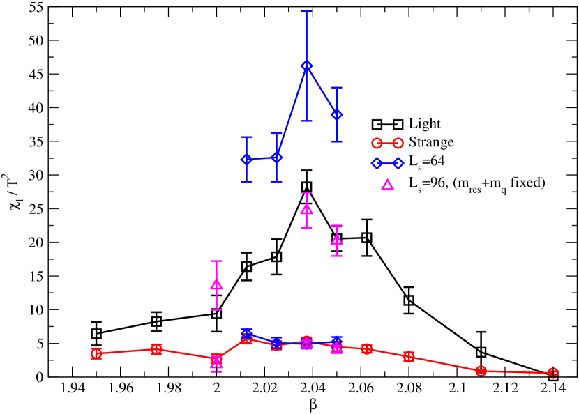
Figure 3: Unitary values for the disconnected chiral susceptibility as well as the results of additional measurements with $L_{s}=64$ and $L_{s}=96$ for the valence quarks.

Figure 6: Values obtained for the Polyakov loop as a function of $\beta$.

Figure 8: The light and strange quark number susceptibilities $c_{2}^{u}$ and $c_{2}^{s}$ plotted as a function of $\beta$.

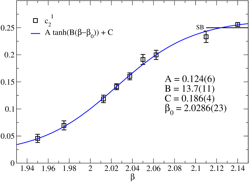
Figure 9: The susceptibilities $c_{2}^{Q}$ and $c_{2}^{I}$ plotted versus $\beta$. The lines show fits based on the hyperbolic ansatz, $f_{I}(\beta)$, given in Eq. 11. The legend also gives the fit parameters, which includes the location of the inflection point, $\beta_{0}$.

References

- (1) A. Bazavov et al., Phys. Rev. D80, 014504 (2009), arXiv:0903.4379 [hep-lat]
- (2) M. Cheng et al., Phys. Rev. D74, 054507 (2006), hep-lat/0608013
- (3) C. Bernard et al. (MILC), Phys. Rev. D71, 034504 (2005), hep-lat/0405029
- (4) Y. Aoki, Z. Fodor, S. D. Katz, and K. K. Szabo, Phys. Lett. B643, 46 (2006), hep-lat/0609068
- (5) P. Chen et al., Phys. Rev. D64, 014503 (2001), hep-lat/0006010
- (6) V. G. Bornyakov et al.(2009), arXiv:0910.2392 [hep-lat]
- (7) D. B. Kaplan, Phys. Lett. B288, 342 (1992), arXiv:hep-lat/9206013
- (8) Y. Shamir, Nucl. Phys. B406, 90 (1993), arXiv:hep-lat/9303005
- (9) V. Furman and Y. Shamir, Nucl. Phys. B439, 54 (1995), arXiv:hep-lat/9405004
- (10) D. J. Antonio et al. (RBC and UKQCD), Phys. Rev. D75, 114501 (2007), arXiv:hep-lat/0612005
- (11) C. Allton et al. (RBC and UKQCD), Phys. Rev. D76, 014504 (2007), arXiv:hep-lat/0701013
- (12) C. W. Bernard et al., Phys. Rev. D62, 034503 (2000), arXiv:hep-lat/0002028
- (13) C. Allton et al. (RBC-UKQCD), Phys. Rev. D78, 114509 (2008), arXiv:0804.0473 [hep-lat]
- (14) D. J. Antonio et al. (RBC), Phys. Rev. D77, 014509 (2008), arXiv:0705.2340 [hep-lat]
- (15) M. A. Clark, A. D. Kennedy, and Z. Sroczynski, Nucl. Phys. Proc. Suppl. 140, 835 (2005), hep-lat/0409133
- (16) M. A. Clark and A. D. Kennedy, Phys. Rev. Lett. 98, 051601 (2007), arXiv:hep-lat/0608015
- (17) P. de Forcrand and O. Philipsen(2006), hep-lat/0607017
- (18) T. Takaishi and P. de Forcrand, Phys. Rev. E73, 036706 (2006), hep-lat/0505020
- (19) M. Cheng et al., Phys. Rev. D77, 014511 (2008), arXiv:0710.0354 [hep-lat]
- (20) S. A. Gottlieb, W. Liu, D. Toussaint, R. L. Renken, and R. L. Sugar, Phys. Rev. Lett. 59, 2247 (1987)
- (21) J. C. R. Bloch and T. Wettig, Phys. Rev. D76, 114511 (2007), arXiv:0709.4630 [hep-lat]
- (22) P. Hegde, F. Karsch, E. Laermann, and S. Shcheredin, Eur. Phys. J. C55, 423 (2008), arXiv:0801.4883 [hep-lat]
- (23) R. V. Gavai and S. Sharma, Phys. Rev. D79, 074502 (2009), arXiv:0811.3026 [hep-lat]
- (24) P. Hasenfratz and F. Karsch, Phys. Lett. B125, 308 (1983)
- (25) P. M. Vranas, Phys. Rev. D57, 1415 (1998), hep-lat/9705023
- (26) P. Hegde, F. Karsch, and C. Schmidt(2008), arXiv:0810.0290 [hep-lat]
- (27) M. Li, PoS LAT2006, 183 (2006), arXiv:hep-lat/0610106
- (28) A. Gray et al., Phys. Rev. D72, 094507 (2005), hep-lat/0507013
- (29) M. Golterman and Y. Shamir, Phys. Rev. D68, 074501 (2003), arXiv:hep-lat/0306002
- (30) M. Golterman, Y. Shamir, and B. Svetitsky, Phys. Rev. D71, 071502 (2005), arXiv:hep-lat/0407021
- (31) M. Golterman, Y. Shamir, and B. Svetitsky, Phys. Rev. D72, 034501 (2005), arXiv:hep-lat/0503037
- (32) J. Gasser and H. Leutwyler, Phys. Lett. B184, 83 (1987)
- (33) P. Hasenfratz and H. Leutwyler, Nucl. Phys. B343, 241 (1990)
- (34) A. V. Smilga and J. Stern, Phys. Lett. B318, 531 (1993)
- (35) A. V. Smilga and J. J. M. Verbaarschot, Phys. Rev. D54, 1087 (1996), arXiv:hep-ph/9511471
- (36) S. Ejiri et al.(2009), arXiv:0909.5122 [hep-lat]
- (37) F. Karsch (RBC-Bielefeld), Nucl. Phys. A820, 99c (2009), arXiv:0810.3078 [hep-lat]
- (38) C. Kelly (RBC and UKQCD), PoS LAT2009, 087 (2009)
- (39) R. Mawhinney (RBC and UKQCD), PoS LAT2009, 081 (2009)
- (40) N. H. Christ and L. L. Wu, Nucl. Phys. Proc. Suppl. 106, 438 (2002)
- (41) Y. Aoki et al., JHEP 06, 088 (2009), arXiv:0903.4155 [hep-lat]
- (42) P. M. Vranas(1999), arXiv:hep-lat/0001006
- (43) P. M. Vranas, Phys. Rev. D74, 034512 (2006), arXiv:hep-lat/0606014
- (44) H. Fukaya et al. (JLQCD), Phys. Rev. D74, 094505 (2006), arXiv:hep-lat/0607020
- (45) D. Renfrew, T. Blum, N. Christ, R. Mawhinney, and P. Vranas(2009), arXiv:0902.2587 [hep-lat]
- (46) R. V. Gavai and S. Sharma(2009), arXiv:0906.5188 [hep-lat]
- (47) M. Cheng et al., Phys. Rev. D79, 074505 (2009), arXiv:0811.1006 [hep-lat]
Acknowledgments
We would like to thank Chulwoo Jung, Christian Schmidt and our other collaborators in the RBC-Bielefeld and HotQCD collaborations for helpful discussions. This work has been carried out on the QCDOC computer at Columbia University and on the computers of the New York Center for Computational Sciences at Stony Brook University/Brookhaven National Laboratory which is supported by the U.S. Department of Energy under Contract No. DE-AC02-98CH10886 and by the State of New York. The work was supported in part by the U.S. Department of Energy under grant number DE-FG02-92ER40699 and contract number DE-AC02-98CH10886.