Relativistic viscous hydrodynamics,
conformal invariance, and holography

Abstract:

We consider second-order viscous hydrodynamics in conformal field theories at finite temperature. We show that conformal invariance imposes powerful constraints on the form of the second-order corrections. By matching to the AdS/CFT calculations of correlators, and to recent results for Bjorken flow obtained by Heller and Janik, we find three (out of five) second-order transport coefficients in the strongly coupled ${\cal N}=4$ supersymmetric Yang-Mills theory. We also discuss how these new coefficents can arise within the kinetic theory of weakly coupled conformal plasmas. We point out that the Müller-Israel-Stewart theory, often used in numerical simulations, does not contain all allowed second-order terms and, frequently, terms required by conformal invariance.

1 Introduction

Relativistic hydrodynamics is an important theoretical tool in heavy-ion physics, astrophysics, and cosmology. Hydrodynamics gives reliable description of the non-equilibrium real-time macroscopic evolution of a given system. It is an effective description in terms of a few relevant variables (fields) and it applies to the evolution which is slow, both in space and in time, relative to a certain microscopic scale [1, 2].

In the most common applications of hydrodynamics the underlying microscopic theory is a kinetic theory. In this case the microscopic scale which limits the validity of hydrodynamics is the mean free path $\ell_{\rm mfp}$. In other words, the parameter controlling the precision of hydrodynamic approximation is $k\ell_{\rm mfp}$, where $k$ is the characteristic momentum scale of the process under consideration.

More generally, the underlying microscopic description is a quantum field theory, which might not necessarily admit a kinetic description. An experimental example of such a system is the strongly coupled quark-gluon plasma (sQGP) recently discovered at the Relativistic Heavy-Ion Collider (RHIC) at Brookhaven National Laboratory. The ${\cal N}=4$ supersymmetric $SU(N_{c})$ Yang-Mills theory in the limit of strong coupling provides a theoretical example of such a system which, in the limit of large number of colors $N_{c}$, can be studied analytically using the AdS/CFT correspondence [3]. In these cases, where kinetic description may be absent, the role of the parameter $\ell_{\rm mfp}$ is played by some typical microscopic scale. In the above examples this scale is set by the temperature: $\ell_{\rm mfp}\sim T^{-1}$.

When the parameter $k\ell_{\rm mfp}$ is not too small, one may want to go beyond the first order in $k\ell_{\rm mfp}$. This is the case, for example, in the early stages of heavy-ion collisions. There are two sources of corrections beyond the $k\ell_{\rm mfp}$ order. First, there are corrections due to thermal fluctuations of hydrodynamic variables contributing via nonlinearities of the hydrodynamic equations. The fluctuation corrections lead to nonanalytic low-momentum behavior of certain correlators [4] (similarly to the chiral logarithms that emerge from loops in chiral perturbation theory) and are, for example, essential for describing non-trivial dynamical critical behavior near phase transitions [5]. Such corrections are calculable in the framework of hydrodynamics with thermal noise.

The second source of corrections are second-order terms (order $(k\ell_{\rm mfp})^{2}$) in the hydrodynamic equations, sometimes called the Burnett corrections [6]. These corrections come with additional transport coefficients. These second-order transport coefficients are not calculable from hydrodynamics, but have to be determined from underlying microscopic description or input phenomenologically, similarly to first-order transport coefficients such as viscosity.

In gauge theories with a large number of colors $N_{c}$ the corrections of the first type (fluctuation) are suppressed by $1/N_{c}^{2}$  [4] and therefore the corrections of the second type (Burnett) dominate in the limit of fixed $k$ and $N_{c}\to\infty$. For this reason, in this paper, we concentrate on the second type of corrections. Moreover, we shall consider the case of conformal theories, where the number of second-order transport coefficients is substantially reduced. In the real-world applications we deal with fluids which are not exactly conformal, however, e.g., QCD at sufficiently high temperatures is approximately conformal.

This paper is organized as follows. In Sec. 2 we derive the consequences of conformal symmetry for hydrodynamics. In Sec. 3 we classify all terms of order $k^{2}$ consistent with conformal symmetry. In Sec. 4 we compute three of the five new transport coefficients for the strongly-coupled ${\cal N}=4$ supersymmetric Yang-Mills (SYM) theory using the AdS/CFT correspondence. In Sec. 5 we show that hydrodynamic equations derived from the kinetic description (Boltzmann equation) of a weakly coupled conformal theory do not contain all allowed second-order terms. In Sec. 6, we analyze our findings from the point of view of the Müller-Israel-Stewart theory [7, 8, 9, 10], which involves only one new parameter at the second order, and show that this parameter cannot account for all second-order corrections. Our conclusions are summarized in Sec. 7.

2 Conformal invariance in hydrodynamics

To set the stage, let us emphasize again that hydrodynamics is a controlled expansion scheme ordered by the power of the parameter $k\ell_{\rm mfp}$, or equivalently, by the number of derivatives of the hydrodynamic fields. We shall set up this expansion paying particular attention to the consequences of the conformal invariance on the equations of hydrodynamics.

2.1 Conformal invariance and Weyl anomalies

The hydrodynamic fields are expectation values of certain quantum fields, such as e.g., components of the stress-energy tensor, averaged over small but macroscopic volumes and time intervals. Such averages can, in principle, be calculated in the close-time-path (CTP) formalism [11]. Consider a generic finite-temperature field theory in the CTP formulation. Turning on external metrics on the upper and lower contours, the partition function is

$$Z[g_{\mu\nu}^{1},g_{\mu\nu}^{2}]=\int\!{\cal D}\phi_{1}\,{\cal D}\phi_{2}\,\exp\left\{iS[\phi_{1},g_{\mu\nu}^{1}]-iS[\phi_{2},g_{\mu\nu}^{2}]\right\},$$ (1)

where $\phi_{1}$ and $\phi_{2}$ represent the two sets of all fields living on the upper and lower parts of the contours, and $S[\phi,g_{\mu\nu}]$ is the general coordinate invariant action.

The one-point Green’s function of the stress-energy tensor is obtained by differentiating the partition function (the metric signature here is $-+++$):

$$\langle T^{1\mu\nu}\rangle =-\frac{2i}{\sqrt{-g_{1}}}\frac{\delta\ln Z}{\delta g_{\mu\nu}^{1}}\,,$$ (2)

$$\langle T^{2\mu\nu}\rangle =\phantom{+}\frac{2i}{\sqrt{-g_{2}}}\frac{\delta\ln Z}{\delta g_{\mu\nu}^{2}}\,,$$ (3)

where $\langle\ldots\rangle$ denote the mean value under the path integral and $\sqrt{-g_{1,2}}\equiv\sqrt{-{\rm det}g_{\mu\nu}^{1,2}}$.

In this paper we consider conformally invariant theories. In such theories the action $S[\phi,g_{\mu\nu}]$ evaluated on classical equations of motion $\delta S/\delta\phi=0$ and viewed as a functional of the external metric $g_{\mu\nu}$ is invariant under local dilatations, or Weyl transformations:

$$g_{\mu\nu}\to e^{-2\omega}g_{\mu\nu},$$ (4)

with parameter $\omega$ a function of space-time coordinates. As a consequence, classical stress-energy tensor $T^{\mu\nu}_{\rm cl}\equiv\delta S/\delta g_{\mu\nu}$ is traceless since $g_{\mu\nu}T^{\mu\nu}_{\rm cl}=-(1/2)\delta S/\delta\omega=0$.

In the conformal quantum theory (1) the Weyl anomaly [12, 13] implies

$$g^{1}_{\mu\nu}\langle T^{1\mu\nu}\rangle =W_{d}[g^{1}_{\mu\nu}],$$ (5a)

$$g^{2}_{\mu\nu}\langle T^{2\mu\nu}\rangle =W_{d}[g^{2}_{\mu\nu}],$$ (5b)

where $W_{d}$ is the Weyl anomaly in $d$ dimensions, which is identically zero for odd $d$. For $d=4$:

$$W_{4}[g_{\mu\nu}]=-\frac{a}{16\pi^{2}}(R_{\mu\nu\lambda\rho}R^{\mu\nu\lambda\rho}-4R_{\mu\nu}R^{\mu\nu}+R^{2})+\frac{c}{16\pi^{2}}(R_{\mu\nu\lambda\rho}R^{\mu\nu\lambda\rho}-2R_{\mu\nu}R^{\mu\nu}+\tfrac{1}{3}R^{2}),$$ (6)

where $R_{\mu\nu\lambda\rho}$ and $R_{\mu\nu}$ ($R$) are the Riemann tensor and Ricci tensor (scalar), and for $SU(N_{c})$ ${\mathcal{N}}=4$ SYM theory $a=c=\frac{1}{4}\left(N_{c}^{2}-1\right)$ [14]. The right-hand side of Eqs. (5) contains four derivatives. In general, for even $d=2k$, $W_{2k}$ contains $2k$ derivatives of the metric.

Let us now explore the consequences of Weyl anomalies for hydrodynamics. The hydrodynamic equations (without noise) do not capture the whole set of CTP Green’s functions, but only the retarded ones. Hydrodynamics determines the stress-energy tensor $T^{\mu\nu}$ (more precisely, its slowly varying average over sufficiently long scales) in the presence of an arbitrary (also slowly varying) source $g_{\mu\nu}$. The connection to the CTP partition function can be made explicit by writing

$$g^{1}_{\mu\nu}=g_{\mu\nu}+\frac{1}{2}\gamma_{\mu\nu},\qquad g^{2}_{\mu\nu}=g_{\mu\nu}-\frac{1}{2}\gamma_{\mu\nu}.$$ (7)

If $\gamma_{\mu\nu}=0$ then $Z=1$ since the time evolution on the lower contour exactly cancels out the time evolution on the upper contour. When $\gamma_{\mu\nu}$ is small one can expand

$$\ln Z=\frac{i}{2}\int\!dx\,\sqrt{-g(x)}\,\gamma_{\mu\nu}(x)T^{\mu\nu}(x)+O(\gamma^{2}),$$ (8)

where $T^{\mu\nu}(x)$ depends on $g_{\mu\nu}$, and is the stress-energy tensor in the presence of the source $g_{\mu\nu}$. At long distance scales it should be the same as computed from hydrodynamics.

Substituting Eqs. (7) and (8) into Eq. (5), the $O(1)$ and $O(\gamma)$ terms yield two equations:

$$g_{\mu\nu}T^{\mu\nu} =W_{d}[g_{\mu\nu}],$$ (9a)

$$g_{\mu\nu}(x)\frac{\delta[\sqrt{-g(x)}\,T^{\alpha\beta}(x)]}{\delta g_{\mu\nu}(y)}+\sqrt{-g(x)}T^{\alpha\beta}(x)\delta^{d}(x-y) =\frac{\delta}{\delta g_{\alpha\beta}(y)}(\sqrt{-g(x)}\,W_{d}[g_{\mu\nu}(x)]).$$ (9b)

In odd dimensions, the right hand sides of Eqs. (9) are zero. In even dimensions, they contain $d$ derivatives. In a hydrodynamic theory, where one keeps less than $d$ derivatives, they can be set to zero. For example, at $d=4$, the Weyl anomaly is visible in hydrodynamics only if one keeps terms to the fourth order in derivatives. This is two orders higher than in second-order hydrodynamics considered in this paper. For larger even $d$, one has to go to even higher orders to see the Weyl anomaly. Thus, we can neglect $W_{d}$ on the right hand side: second-order hydrodynamic theory is invariant under Weyl transformations. The two conditions (9) then become

$$g_{\mu\nu}T^{\mu\nu} =0,$$ (10)

$$g_{\mu\nu}\frac{\delta T^{\alpha\beta}(y)}{\delta g_{\mu\nu}(x)} =-\left(\frac{d}{2}+1\right)\delta^{d}(x-y)T^{\alpha\beta}(x).$$ (11)

Since the r.h.s. of equation (11) is $-(1/2)\delta T^{\mu\nu}/\delta\omega$ it implies the following tranformation law for $T^{\mu\nu}$ under Weyl transformations (4):

$$T^{\mu\nu}\to e^{(d+2)\omega}\,T^{\mu\nu}.$$ (12)

Noting that $\ln Z$ is invariant under Weyl transformations this could have been gleaned from Eq. (8) already.

A simple rule of thumb is that for tensors transforming homogeneously

$$A^{\mu_{1}\ldots\mu_{m}}_{\nu_{1}\ldots\nu_{n}}\to e^{\Delta_{A}\,\omega}A^{\mu_{1}\ldots\mu_{m}}_{\nu_{1}\ldots\nu_{n}},$$ (13)

the conformal weight $\Delta_{A}$ equals the mass dimension plus the difference between the number of contravariant and covariant indices:

$$\Delta_{A}=[A]+m-n.$$ (14)

2.2 First order hydrodynamics as derivative expansion

The existence of hydrodynamic description owes itself to the presence of conserved quantities, whose densities can evolve (oscillate or relax to equilibrium) at arbitrarily long times provided the fluctuations are of large spatial size. Correspondingly, the expectation values of such densities are the hydrodynamic fields.

In the simplest case we shall consider here, i.e., in a theory without conserved charges, there are 4 such hydrodynamic fields: energy density $T^{00}$ and 3 components of the momentum density $T^{0i}$. It is common and convenient to use the local velocity $u^{\mu}$ instead of the momentum density variable. It can be defined as the boost velocity needed to go from the local rest frame, where the momentum density $T^{0i}$ vanishes, back to the lab frame. Similarly, it is convenient to use $\varepsilon$ – the energy density in the local rest frame – instead of the $T^{00}$ in the lab frame. The 4 equations for thus defined variables $\varepsilon$ and $u^{\mu}$ are conservation equations of the energy-momentum tensor $\nabla_{\mu}T^{\mu\nu}=0$.

In a covariant form the above definitions of $\varepsilon$ and $u^{\mu}$ can be summarized as

$$T^{\mu\nu}=\varepsilon\,u^{\mu}u^{\nu}+T^{\mu\nu}_{\perp}.$$ (15)

In hydrodynamics, the remaining components $T^{\mu\nu}_{\perp}$ (spatial in the local rest frame: $u_{\mu}T^{\mu\nu}_{\perp}=0$) of the stress-energy tensor $T^{\mu\nu}$ appearing in the conservation equations are not independent variables, but rather instantaneous functions of the hydrodynamic variables $\varepsilon$ and $u^{\mu}$ and their derivatives. In the hydrodynamic limit, this is the consequence of the fact that the hydrodynamic modes are infinitely slower than all other modes, the latter therefore can be integrated out. All quantities appearing in hydrodynamic equations are averaged over these fast modes, and are functions of the slow varying hydrodynamic variables. The functional dependence of $T^{\mu\nu}_{\perp}$ (constituitive equations) can be expanded in powers of derivatives of $\varepsilon$ and $u^{\mu}$.

Writing the most general form of this expansion consistent with symmetries gives, up to 1st order in derivatives,

$$T^{\mu\nu}_{\perp}=P(\varepsilon)\Delta^{\mu\nu}-\eta(\varepsilon)\sigma^{\mu\nu}-\zeta(\varepsilon)\Delta^{\mu\nu}(\nabla{\cdot}u),$$ (16)

where the symmetric, transverse tensor with no derivatives $\Delta^{\mu\nu}$ is given by

$$\Delta^{\mu\nu}=g^{\mu\nu}+u^{\mu}u^{\nu}\,.$$ (17)

In the local rest frame it is the projector on the spatial subspace. The symmetric, transverse and traceless tensor of first derivatives $\sigma^{\mu\nu}$ is defined by

$$\sigma^{\mu\nu}=2{}^{\langle}\nabla^{\mu}u^{\nu}{}^{\rangle}\,,$$ (18)

where for a second rank tensor $A^{\mu\nu}$ the tensor defined as

$${}^{\langle}A^{\mu\nu}{}^{\rangle}\equiv\frac{1}{2}\Delta^{\mu\alpha}\Delta^{\nu\beta}(A_{\alpha\beta}+A_{\beta\alpha})-\frac{1}{d-1}\Delta^{\mu\nu}\Delta^{\alpha\beta}A_{\alpha\beta}\,\equiv A^{\langle\mu\nu\rangle}$$ (19)

is transverse $u_{\mu}A^{\langle\mu\nu\rangle}=0$ (i.e., only spatial components in the local rest frame are nonzero) and traceless $g_{\mu\nu}A^{\langle\mu\nu\rangle}=0$.

In the gradient expansion (16), the scalar function $P(\varepsilon)$ can be identified as the thermodynamic pressure (in equilibrium, when all the gradients vanish), while $\eta(\varepsilon)$ and $\zeta(\varepsilon)$ are the shear and bulk viscosities. The expansion coefficients $P$, $\eta$ and $\zeta$ are determined by the physics of the fast (non-hydrodynamic, microscopic) modes that have been integrated out.

2.3 Conformal invariance in first-order hydrodynamics

It is straightforward to check that if $T^{\mu\nu}$ transforms as in Eq. (12) and $T^{\mu}_{\mu}=0$, then its covariant divergence transforms homogeneously: $\nabla_{\mu}T^{\mu\nu}\to e^{(d+2)\omega}\nabla_{\mu}T^{\mu\nu}$, hence the hydrodynamic equation $\nabla_{\mu}T^{\mu\nu}=0$ is Weyl invariant [15].

Let us now see what restrictions conformal invariance imposes on the first-order constitutive equations (16). First, the tracelessness condition $T^{\mu}_{\mu}=0$ forces $\varepsilon=(d-1)P$ and $\zeta=0$. Since in a conformal theory $\varepsilon={\rm const}{\cdot}T^{d}$, we shall trade $\varepsilon$ variable for $T$ in what follows. Since $g_{\mu\nu}u^{\mu}u^{\nu}=-1$ the conformal weight of $u^{\mu}$ is 1. By definition (15) and by (12) $\varepsilon$ has conformal weight $d$ and therefore

$$T\to e^{\omega}T,\qquad u^{\mu}\to e^{\omega}u^{\mu}$$ (20)

in accordance with the simple rule (14).

By direct computation we find that

$$\sigma^{\mu\nu}\to e^{3\omega}\sigma^{\mu\nu},$$ (21)

i.e. $\sigma^{\mu\nu}$ transforms homogeneously with conformal weight 3 independent of $d$ (in agreement with (14)). For conformal fluids $\eta={\rm const}\cdot T^{d-1}$, and therefore $T^{\mu\nu}$ transforms homogeneously under Weyl transformation as in Eq. (12).

3 Second-order hydrodynamics of a conformal fluid

In this Section we shall continue the derivative expansion (16). We shall write down all possible second-order terms in the stress-energy tensor allowed by Weyl invariance. Then we shall compute the coefficients in front of these terms in the ${\cal N}=4$ SYM plasma by matching hydrodynamic correlation functions with gravity calculations in Section 4.

3.1 Second-order terms

Rewriting Eq. (15) we introduce the dissipative part of the stress-energy tensor, $\Pi^{\mu\nu}$:

$$T^{\mu\nu}=\varepsilon u^{\mu}u^{\nu}+P\Delta^{\mu\nu}+\Pi^{\mu\nu}\,,$$ (22)

which contains only the derivatives and vanishes in a homogeneous equilibrium state. The tensor $\Pi^{\mu\nu}$ is symmetric and transverse, $u_{\mu}\Pi^{\mu\nu}=0$. For conformal fluids it must be also traceless $g_{\mu\nu}\Pi^{\mu\nu}=0$. To first order

$$\Pi^{\mu\nu}=-\eta\sigma^{\mu\nu}+\textrm{(2nd order terms)},$$ (23)

where $\sigma^{\mu\nu}$ is defined in Eq. (18). We will also use the notation for the vorticity

$$\Omega^{\mu\nu}=\frac{1}{2}\Delta^{\mu\alpha}\Delta^{\nu\beta}(\nabla_{\alpha}u_{\beta}-\nabla_{\beta}u_{\alpha})\,.$$ (24)

We note that in writing down second-order terms in $\Pi^{\mu\nu}$, one can always rewrite the derivatives along the $d$-velocity direction

$$D\equiv u^{\mu}\nabla_{\mu}$$ (25)

(temporal derivative in the local rest frame) in terms of transverse (spatial in the local rest frame) derivatives through the zeroth-order equations of motion:

$$D\ln T=-\frac{1}{d-1}(\nabla_{\perp}\cdot u),\quad Du^{\mu}=-\nabla_{\perp}^{\mu}\ln T,\qquad\nabla^{\mu}_{\perp}\equiv\Delta^{\mu\alpha}\nabla_{\alpha}\,.$$ (26)

Notice also that $\nabla_{\perp}\!\cdot u=\nabla\cdot u$.

With the restriction of transversality and tracelessness, there are eight possible contributions to the stress-energy tensor:

$$\begin{split}&\nabla^{\langle\mu}\ln T\,\nabla^{\nu\rangle}\ln T,\quad\nabla^{\langle\mu}\nabla^{\nu\rangle}\ln T,\quad\sigma^{\mu\nu}(\nabla{\cdot}u),\quad{\sigma^{\langle\mu}}_{\lambda}\sigma^{\nu\rangle\lambda}\\ &{\sigma^{\langle\mu}}_{\lambda}\Omega^{\nu\rangle\lambda},\quad{\Omega^{\langle\mu}}_{\lambda}\Omega^{\nu\rangle\lambda},\quad u_{\alpha}R^{\alpha\langle\mu\nu\rangle\beta}u_{\beta},\quad R^{\langle\mu\nu\rangle}\,.\end{split}$$ (27)

By direct computations we find that there are only five combinations that transform homogeneously under Weyl tranformations. They are

$${\cal O}_{1}^{\mu\nu}=R^{\langle\mu\nu\rangle}-(d-2)\left(\nabla^{\langle\mu}\nabla^{\nu\rangle}\ln T-\nabla^{\langle\mu}\ln T\,\nabla^{\nu\rangle}\ln T\right),$$ (28)

$${\cal O}_{2}^{\mu\nu}=R^{\langle\mu\nu\rangle}-(d-2)u_{\alpha}R^{\alpha\langle\mu\nu\rangle\beta}u_{\beta}\,,$$ (29)

$${\cal O}_{3}^{\mu\nu}={\sigma^{\langle\mu}}_{\lambda}\sigma^{\nu\rangle\lambda}\,,\qquad{\cal O}_{4}^{\mu\nu}={\sigma^{\langle\mu}}_{\lambda}\Omega^{\nu\rangle\lambda}\,,\qquad{\cal O}_{5}^{\mu\nu}={\Omega^{\langle\mu}}_{\lambda}\Omega^{\nu\rangle\lambda}\,.$$ (30)

In the linearized hydrodynamics in flat space only the term ${\cal O}_{1}^{\mu\nu}$ contributes. For convenience and to facilitate the comparision with the Israel-Stewart theory we shall use instead of (28) the term

$${}^{\langle}D\sigma^{\mu\nu}{}^{\rangle}+\frac{1}{d-1}\sigma^{\mu\nu}(\nabla{\cdot}u)$$ (31)

which, with (26), reduces to the linear combination: ${\cal O}_{1}^{\mu\nu}-{\cal O}_{2}^{\mu\nu}-(1/2){\cal O}_{3}^{\mu\nu}-2{\cal O}_{5}^{\mu\nu}$. It is straightforward to check directly that (31) transforms homogeneously under Weyl transformations.

Thus, our final expression for the dissipative part of the stress-energy tensor, up to second order in derivatives, is

$$\begin{split}\Pi^{\mu\nu}&=-\eta\sigma^{\mu\nu}\\ &\quad+\eta\tau_{\Pi}\left[{}^{\langle}D\sigma^{\mu\nu}{}^{\rangle}+\frac{1}{d-1}\sigma^{\mu\nu}(\nabla{\cdot}u)\right]+\kappa\left[R^{\langle\mu\nu\rangle}-(d-2)u_{\alpha}R^{\alpha\langle\mu\nu\rangle\beta}u_{\beta}\right]\\ &\quad+\lambda_{1}{\sigma^{\langle\mu}}_{\lambda}\sigma^{\nu\rangle\lambda}+\lambda_{2}{\sigma^{\langle\mu}}_{\lambda}\Omega^{\nu\rangle\lambda}+\lambda_{3}{\Omega^{\langle\mu}}_{\lambda}\Omega^{\nu\rangle\lambda}\,.\end{split}$$ (32)

The five new constants are $\tau_{\Pi}$, $\kappa$, $\lambda_{1,2,3}$. Note that using lowest order relations $\Pi^{\mu\nu}=-\eta\sigma^{\mu\nu}$, Eqs.(26) and $D\eta=-\eta\,\nabla{\cdot}u$, Eq. (32) may be rewritten in the form

$$\begin{split}\Pi^{\mu\nu}&=-\eta\sigma^{\mu\nu}-\tau_{\Pi}\left[{}^{\langle}D\Pi^{\mu\nu}{}^{\rangle}+\frac{d}{d-1}\Pi^{\mu\nu}(\nabla{\cdot}u)\right]\\ &\quad+\kappa\left[R^{\langle\mu\nu\rangle}-(d-2)u_{\alpha}R^{\alpha\langle\mu\nu\rangle\beta}u_{\beta}\right]\\ &+\frac{\lambda_{1}}{\eta^{2}}{\Pi^{\langle\mu}}_{\lambda}\Pi^{\nu\rangle\lambda}-\frac{\lambda_{2}}{\eta}{\Pi^{\langle\mu}}_{\lambda}\Omega^{\nu\rangle\lambda}+\lambda_{3}{\Omega^{\langle\mu}}_{\lambda}\Omega^{\nu\rangle\lambda}\,.\end{split}$$ (33)

This equation is, in form, similar to an equation of the Israel-Stewart theory (see Section 6). In the linear regime it actually coincides with the Israel-Stewart theory (105). We emphasize, however, that one cannot claim that Eq. (33) captures all orders in the momentum expansion (see Section 6).

Further remarks are in order. First, the $\kappa$ term vanishes in flat space. If one is interested in solving the hydrodynamic equation in flat space, then $\kappa$ is not needed. Nevertheless, $\kappa$ contributes to the two-point Green’s function of the stress-energy tensor. We emphasize that the term proportional to $\kappa$ is not a contact term, since it contains $u^{\mu}$. The $\lambda_{1,2,3}$ terms are nonlinear in velocity, so are not needed if one is looking at small perturbations (like sound waves). For irrotational flows $\lambda_{2,3}$ are not needed. The parameter $\tau_{\Pi}$ has dimension of time and can be thought of as the relaxation time. This interpretation of $\tau_{\Pi}$ can be most clearly seen from Eq. (33). For further discussion, see Section 6.

3.2 Kubo’s formulas

To relate the new kinetic coefficients with thermal correlators, first let us consider the response of the fluid to small and smooth metric perturbations. We shall moreover restrict ourselves to a particular type of perturbations which is simplest to treat using AdS/CFT correspondence. Namely, for dimensions $d\geq 4$ we take $h_{xy}=h_{xy}(t,z)$. For $d=3$, there are only two spatial coordinates, so we take $h_{xy}=h_{xy}(t)$. Since it is a tensor perturbation the fluid remains at rest: $T=\textrm{const}$, $u^{\mu}=(1,{\bf 0})$. Inserting this into Eq. (32) we find, for $d\geq 4$,

$$T^{xy}=-Ph_{xy}-\eta\dot{h}_{xy}+\eta\tau_{\Pi}\ddot{h}_{xy}-\frac{\kappa}{2}[(d-3)\ddot{h}_{xy}+\partial_{z}^{2}h_{xy}]\,.$$ (34)

The linear response theory implies that the retarded Green’s function in the tensor channel is

$$G_{R}^{xy,xy}(\omega,k)=P-i\eta\omega+\eta\tau_{\Pi}\omega^{2}-\frac{\kappa}{2}[(d-3)\omega^{2}+k^{2}]\,.$$ (35)

For $d=3$ there is no momentum $k$, and the formula becomes

$$G_{R}^{xy,xy}(\omega)=P-i\eta\omega+\eta\tau_{\Pi}\omega^{2},\qquad d=3\,.$$ (36)

Thus the two kinetic coefficients $\tau_{\Pi}$ and $\kappa$ can be found from the coefficients of the $\omega^{2}$ and $k^{2}$ terms in the low-momentum expansion of $G_{R}^{xy,xy}(\omega,k)$ in the case of $d\geq 4$, and just from the $\omega^{2}$ term in the case of $d=3$.

3.3 Sound Pole

We now turn to another way to determine $\tau_{\Pi}$, which is based on the position of the sound pole. The fact that we have two independent methods to determine $\tau_{\Pi}$ allows us to check the self-consistency of the calculations.

To obtain the dispersion relation, we consider a (conformal) hydrodynamic system in stationary equilibrium, that is, with fluid velocity $u^{\mu}=(1,{\bf 0})$, homogeneous energy density $\varepsilon={\rm const}\cdot T^{d}$ and $\Pi^{\mu\nu}=0$. The speed of sound is defined by $c_{s}^{2}=dP(\varepsilon)/d\varepsilon$. In conformal theory it is a constant: $c_{s}^{2}=1/(d-1)$. Now let us slightly perturb the system and denote the departure from equilibrium energy density, velocity, and stress as $\delta\varepsilon$, $u^{i}$, and $\Pi^{ij}$.

For small perturbations, one can neglect the nonlinear terms in Eq. (33) and the hydrodynamic equations are identical to those of the Israel-Stewart theory. For completeness, we rederive here the sound dispersion in this theory. To linear approximation in the perturbations, we have

$$\delta T^{00}=\delta\varepsilon,\quad\delta T^{0i}=(\varepsilon+P)u^{i},\quad\delta T^{ij}=c_{s}^{2}\delta\varepsilon\ \delta^{ij}+\Pi^{ij}.$$ (37)

For sound waves travelling in $x$ direction we take $u^{x}$ and $\Pi^{xx}$ as the only nonzero components of $u^{i}$ and $\Pi^{ij}$, and dependent only on $x$ and $t$. Energy-momentum conservation implies

$$\partial_{0}(\delta\varepsilon)+(\varepsilon+P)\partial_{x}u^{x} =0\,,$$ (38)

$$(\varepsilon+P)\partial_{0}u^{x}+c_{s}^{2}\partial_{x}(\delta\varepsilon)+\partial_{x}\Pi^{xx} =0\,.$$ (39)

Eq. (33) has the form

$$\tau_{\Pi}\partial_{0}\Pi^{xx}+\Pi^{xx}=-\frac{2(d-2)}{d-1}\eta\partial_{x}u^{x}\,.$$ (40)

For a plane wave, equations (38), (39) and (40) give the dispersion relation

$$-\omega^{3}\tau_{\Pi}-i\omega^{2}+\omega k^{2}c_{s}^{2}\tau_{\Pi}+\omega k^{2}\frac{2(d-2)}{d-1}\frac{\eta}{\varepsilon+P}+ik^{2}c_{s}^{2}=0.$$ (41)

At small $k$, the two solutions of this equation corresponding to the sound wave are

$$\omega_{1,2}=\pm c_{s}k-i\Gamma k^{2}\pm\frac{\Gamma}{c_{s}}\left(c_{s}^{2}\tau_{\Pi}-\frac{\Gamma}{2}\right)k^{3}+{\cal O}(k^{4})\,,$$ (42)

where

$$\Gamma=\frac{d-2}{d-1}\,\frac{\eta}{\varepsilon+P}\,.$$ (43)

The third solution is given by

$$\omega_{3}=-i\tau_{\Pi}^{-1}+O(k^{2})\,.$$ (44)

Since $\omega_{3}$ does not vanish as $k\to 0$, but remains on the order of a macroscopic scale, this third solution lies beyond the regime of validity of hydrodynamics (see also discussion in Section 6).

3.4 Shear pole

In hydrodynamics, there exists an overdamped mode describing fluid flow in a direction perpendicular to the velocity gradient, e.g., with $u_{y}\sim e^{-i\omega t+ikx}$. First-order hydrodynamics gives the leading-order dispersion relation, $\omega=-i\eta k^{2}/(\varepsilon+P)$. The next correction to this dispersion relation is proportional to $k^{4}$ and thus is beyond the reach of the second-order theory. This correction can be fully determined only in third-order hydrodynamics. To illustrate that, we shall compute this correction here, taking the second-order theory literally and pretending the third-order terms are not contributing. We shall than find the expected mismatch between this (incorrect) result and the AdS/CFT computation in the strongly coupled ${\cal N}=4$ SYM theory.

The perturbation corresponding to the fluid flowing in the $y$ direction with velocity gradient along the $x$ direction (shear flow) involves the variables

$$u^{y}(t,x),\qquad\Pi^{xy}(t,x)\,,$$ (45)

such that we get from $\partial_{\mu}\delta T^{\mu\nu}=0$

$$(\varepsilon+P)\partial_{0}u^{y}+\partial_{x}\Pi^{xy} = 0.$$ (46)

From Eq. (33) we find

$$\tau_{\Pi}\partial_{0}\Pi^{xy}+\Pi^{xy}=-\eta\partial_{x}u^{y}.$$ (47)

The dispersion relation is determined by

$$-\omega^{2}\tau_{\Pi}-i\omega+k^{2}\frac{\eta}{\varepsilon+P}=0$$ (48)

so the shear mode dispersion relation in the limit $k\rightarrow 0$ becomes

$$\omega=-ihk^{2}-ih^{2}{\tau_{\Pi}}k^{4}+\mathcal{O}(k^{6}),\qquad h=\frac{\eta}{\varepsilon+P}\,.$$ (49)

The second solution, $\omega=-i\tau_{\Pi}^{-1}+O(k^{2})$, is obviously beyond the regime of validity of the hydrodynamic equation (see also Section 6).

It is easy to see that expression (49) unjustifiably exceeds the precision of the second-order theory: the kept correction is ${\cal O}(k^{2})$ relative to the leading-order term, instead of being $O(k)$. We can trace this to Eq. (48), in which we keep terms to second order in $\omega$ and $k$. For shear modes, however, $\omega\sim k^{2}$, and the term $\omega^{2}$ that we keep in Eq. (48) is of the same order of magnitude as terms $O(k^{4})$ omitted in Eq. (48). The latter term can appear if the equation (47) for $\Pi^{xy}$ contains a term $\partial_{x}^{3}u^{y}$ that may appear in third-order hydrodynamics. This is beyond the scope of this paper.

3.5 Bjorken Flow

So far, we have studied only quantities involved in the linear response of the fluid, for which linearized hydrodynamics suffices. In order to determine the coefficients $\lambda_{1,2,3}$, one must consider nonlinear solutions to the hydrodynamic equations. One such solution is the Bjorken boost-invariant flow [16], relevant to relativistic heavy-ion collisions.

Since hydrodynamic equations are boost-invariant, a solution with boost-invariant initial conditions will remain boost invariant. The motion in the Bjorken flow is a one-dimensional expansion, along an axis which we choose to be $z$, with local velocity equal to $z/t$. The most convenient are the comoving coordinates: proper time for each local element $\tau=\sqrt{t^{2}-z^{2}}$ and rapidity $\xi={\rm arctanh}\,(z/t)$. In these coordinates each element is at rest: $(u^{\tau},u^{\xi},\bm{u}^{\perp})=(1,0,\bm{0})$.

The motion is irrotational, and thus we can only determine the coefficient $\lambda_{1}$, but not $\lambda_{2}$ or $\lambda_{3}$.

Since velocity $u^{\mu}$ is constant in the coordinates we chose, the only nontrivial equation is the equation for the energy density:

$$D\varepsilon+(\varepsilon+P)\nabla\cdot u+\Pi^{\mu\nu}\nabla_{\mu}u_{\nu}=0.$$ (50)

Boost invariance means that $\varepsilon(\tau)$ is a function of $\tau$ only. The metric is given by $ds^{2}=-d\tau^{2}+\tau^{2}d\xi^{2}+d\bm{x}_{\perp}^{2}$ and it is easy to see that the only nonzero component of $\nabla_{\mu}u_{\nu}$ is $\nabla_{\xi}u_{\xi}=\tau$. Using $P=\varepsilon/(d-1)$ we can write:

$$\partial_{\tau}\varepsilon+\frac{d}{d{-}1}\,\frac{\varepsilon}{\tau}=-\tau\,\Pi^{\xi\xi}.$$ (51)

For large $\tau$, the viscous contribution on the r.h.s. in (51) becomes negligible and the asymptotics of the solution is thus given by

$$\varepsilon(\tau)=C\,\tau^{-2+\nu}+\textrm{(viscous corrections)},\quad\textrm{where}\quad\nu\equiv\frac{d-2}{d-1},$$ (52)

and $C$ is the integration constant. As we shall see, the expansion parameter in (52) is $\tau^{-\nu}$.

Calculating the r.h.s. of Eq. (51) using Eq. (32) we find

$$-\tau\,\Pi^{\xi\xi}=2\nu\eta\tau^{-2}+2\nu^{2}\left(\eta\tau_{\Pi}-2\lambda_{1}\,\frac{d{-}3}{d{-}2}\right)\tau^{-3}+\ldots\,.$$ (53)

Integrating equation (51), one should take into account the fact that kinetic coefficients $\eta$, $\tau_{\Pi}$ and $\lambda_{1}$ in Eq. (53) are functions of $\varepsilon$, which in a conformal theory are given by the following power laws:

$$\eta=C\eta_{0}\left(\frac{\varepsilon}{C}\right)^{(d-1)/d},\qquad\tau_{\Pi}=\tau_{\Pi}^{0}\left(\frac{\varepsilon}{C}\right)^{-1/d},\qquad\lambda_{1}=C\lambda_{1}^{0}\left(\frac{\varepsilon}{C}\right)^{(d-2)/d}\,,$$ (54)

where, for convenience, we defined constants $\eta_{0}$, $\tau_{\Pi}^{0}$ and $\lambda_{1}^{0}$, and we chose the constant $C$ to be the same as in Eq. (52). Integrating Eq. (51) we thus find

$$\frac{\varepsilon(\tau)}{C}=\tau^{-2+\nu}-2\eta_{0}\,\tau^{-2}+\left[\frac{2(d{-}1)}{d}\eta_{0}^{2}-\frac{d{-}2}{d{-}1}\left(\eta_{0}\tau_{\Pi}^{0}-2\lambda_{1}^{0}\,\frac{d{-}3}{d{-}2}\right)\right]\tau^{-2-\nu}+\ldots\,.$$ (55)

In Section 4.4 we shall match the Bjorken flow solution in the strongly-coupled ${\cal N}=4$ SYM theory found in [17] (see also [18]) using AdS/CFT correspondence and determine $\lambda_{1}$ in this theory.

In order to compare our results to the ones obtained in Ref. [17], we shall write here the equations of second-order hydrodynamics using also the alternative representation (33) for $\Pi^{\xi\xi}$ in (51). We obtain the following system of equations for the energy density and the component of the viscous flow, which we define as $\Phi\equiv-\Pi^{\xi}_{\xi}$ (see [19]; c.f. [20] for $\lambda_{1}=0$):

$$\partial_{\tau}\varepsilon = -\frac{d}{d{-}1}\frac{\varepsilon}{\tau}+\frac{\Phi}{\tau}\,,$$ (56)

$$\tau_{\Pi}\partial_{\tau}\Phi = \frac{2(d{-}2)}{d{-}1}\frac{\eta}{\tau}-\Phi-\frac{d}{d-1}\frac{\tau_{\Pi}}{\tau}\,\Phi-\frac{d{-}3}{d{-}2}\,\frac{\lambda_{1}}{\eta^{2}}\,\Phi^{2}\,.$$ (57)

As should be expected, the asymptotics of the solution of this system coincides with Eq. (55). Equation (57) is different from the one used in [17] by the last two terms proportional to $\tau_{\Pi}$ and $\lambda_{1}$.

4 Second-order hydrodynamics for strongly coupled ${\cal N}=4$ supersymmetric Yang-Mills plasma

In this Section, we compute the parameters $\tau_{\Pi}$, $\kappa$, and $\lambda_{1}$ of the second-order hydrodynamics for a theory whose gravity dual is well-known: ${\cal N}=4$ SU($N_{c}$) supersymmetric Yang-Mills theory in the limit $N_{c}\rightarrow\infty$, $g^{2}N_{c}\rightarrow\infty$ [3, 21, 22]. According to the gauge/gravity duality conjecture, in this limit the theory at finite temperature $T$ has an effective description in terms of the AdS-Schwarzschild gravitational background with metric

$$ds^{2}_{5}={\pi^{2}T^{2}L^{2}\over u}\left(-f(u)dt^{2}+dx^{2}+dy^{2}+dz^{2}\right)+{L^{2}\over 4f(u)u^{2}}du^{2}\,,$$ (58)

where $f(u)=1-u^{2}$, and $L$ is the AdS curvature scale [14]. The duality allows one to compute the retarded correlation functions of the gauge-invariant operators at finite temperature. The result of such a computation would in principle be exact in the full microscopic theory (in the limit $N_{c}\rightarrow\infty$, $g^{2}N_{c}\rightarrow\infty$). As we are interested in the hydrodynamic limit of the theory, here we compute the correlators in the form of low-frequency, long-wavelength expansions. In momentum space, the dimensionless expansion parameters are

$$\textswab{w}=\frac{\omega}{2\pi T}\ll 1,\qquad\textswab{q}\equiv\frac{k}{2\pi T}\ll 1.$$ (59)

Comparing these expansions to the predictions of the second-order hydrodynamics obtained in Sections 3.2, 3.3 and 3.5 for $d=4$, we can read off the coefficients $\tau_{\Pi}$, $\kappa$, $\lambda_{1}$.

One must be aware that the ${\cal N}=4$ SU($N_{c}$) supersymmetric Yang-Mills theory posesses conserved $R$-charges, corresponding to SO(6) global symmetry. Therefore, complete hydrodynamics of this theory must involve additional hydrodynamic degrees of freedom – $R$-charge densities. Our discussion of generic conformal hydrodynamics without conserved charges can be, of course, generalized to this case. This is beyond the scope of this paper. Here we only need to observe that since the $R$-charge densities are not singlets under the SO(6) they cannot contribute at linear order to the equations for $T^{\mu\nu}$. These contributions are therefore irrelevant for the linearized hydrodynamics we consider in Sections 3.2, 3.3 and 3.4. For the discussion of the Bjorken flow in Section 3.5 they are also irrelevant, since (and as long as) we consider solutions with zero $R$-charge density.

4.1 Scalar channel

We start by computing the low-momentum expansion of the correlator $G^{R}_{xy,xy}(\omega,k)$. To leading order in momentum, this correlation function has been previously computed from gravity in [23, 24]. Following [24], here we obtain the next to leading order term in the expansion.

The relevant fluctuation of the background metric (58) is the component $\phi\equiv h_{x}^{y}$ of the graviton. The retarded correlator in momentum space is determined by the on-shell boundary action

$$S_{tot}[H_{0},k]=\lim_{\epsilon\rightarrow 0}\Biggl{(}S_{boundary}^{grav}[H_{0},\epsilon,k]+S_{c.t.}[H_{0},\epsilon,k]\Biggr{)}\,,$$ (60)

following the prescription formulated in [23]. Here $H_{0}(k)=H(\epsilon,k)$ is the boundary value (more precisely, the value at the cutoff $u=\epsilon\rightarrow 0$) of the solution to the graviton’s equation of motion (Eq. (6.6) in [24])

$$H(u,k)=H_{0}(k)\frac{\phi_{k}(u)}{\phi_{k}(\epsilon)}\,.$$ (61)

A perturbative solution $\phi_{k}(u)$ to order $\textswab{w}^{2}$, $\textswab{q}^{2}$ is given by Eq. (6.8) in [24]. The gravitational action (Eq. (6.4) in [24]) reduces to the sum of two terms, the horizon contribution and the boundary contribution. The horizon contribution should be discarded, as explained in [23] and later justified in [25]. The remaining boundary term, $S_{boundary}^{grav}[H_{0},\epsilon,k]$, is divergent in the limit $\epsilon\rightarrow 0$, and should be supplemented by the counterterm action $S_{c.t.}[H_{0},\epsilon,k]$ following a procedure known as the holographic renormalization. In the case of gravitational fluctuations, the counterterm action is [27]

$$S_{ct}=-\frac{3N_{c}^{2}}{4\pi^{2}L^{4}}\int\limits_{u=\epsilon}d^{4}x\sqrt{-\gamma}\Biggl{(}1+\frac{L^{2}}{2}P-\frac{L^{4}}{12}\left(P^{kl}P_{kl}-P^{2}\right)\,\log{\epsilon}\Biggr{)}\,,$$ (62)

where $\gamma_{ij}$ is the metric (58) restricted to $u=\epsilon$, and

$$P=\gamma^{ij}P_{ij}\,,\qquad P_{ij}=\frac{1}{2}\Biggl{(}R_{ij}-\frac{1}{6}R\gamma_{ij}\Biggr{)}\,.$$ (63)

Evaluating (62), we find the total boundary action

$$S_{tot}=-\frac{\pi^{2}N_{c}^{2}T^{4}}{8}\Biggl{(}V_{4}-\frac{H(\epsilon)H^{\prime}(\epsilon)}{\epsilon}+\frac{H^{2}(\epsilon)}{2}-\frac{(\textswab{q}^{2}-\textswab{w}^{2})H^{2}(\epsilon)}{\epsilon}\Biggr{)}+O(\textswab{w}^{3},\textswab{w}\textswab{q}^{2})+O(\epsilon)\,.$$ (64)

The boundary action (64) is finite in the limit $\epsilon\rightarrow 0$. Its fluctuation-independent part is $S_{tot}^{0}=-PV_{4}$, where $P=\pi^{2}N_{c}^{2}T^{4}/8$ is the pressure in ${\cal N}=4$ SYM, $V_{4}$ is the four-volume. The part quadratic in fluctuations gives the two-point function. Substituting the solution (61) into Eq. (64) and using the recipe of [23], we find

$$G_{xy,xy}^{R}=-\frac{\pi^{2}N_{c}^{2}T^{4}}{4}\Biggl{[}i\textswab{w}-\textswab{w}^{2}+\textswab{q}^{2}+\textswab{w}^{2}\ln{2}-\frac{1}{2}\Biggr{]}+O(\textswab{w}^{3},\textswab{w}\textswab{q}^{2})\,.$$ (65)

Comparing Eq. (65) to the hydrodynamic result (35) we obtain the pressure [28], the viscosity [29] and the two parameters of the second-order hydrodynamics for ${\cal N}=4$ SYM:

$$P=\frac{\pi^{2}}{8}N_{c}^{2}T^{4},\quad\eta=\frac{\pi}{8}N_{c}^{2}T^{3},\,\quad\tau_{\Pi}=\frac{2-\ln 2}{2\pi T}\,,\quad\kappa=\frac{\eta}{\pi T}\,.$$ (66)

4.2 Shear channel

The dispersion relation (49) manifests itself as a pole in the retarded Green’s functions $G^{R}_{ty,ty}$, $G^{R}_{ty,xy}$, $G^{R}_{xy,xy}$ in the hydrodynamic approximation. To quadratic order in $k$ this dispersion relation was computed from dual gravity in Section 6.2 of Ref. [24]. Here we extend that calculation to quartic order in $k$. This amounts to solving the differential equation for the gravitational fluctuation $G(u)$ [24]

$$G^{\prime\prime}-\left({2u\over f}-{i\textswab{w}\over 1-u}\right)G^{\prime}+\frac{1}{f}\biggl{(}2+{i\textswab{w}\over 2}-{\textswab{q}^{2}\over u}+{\textswab{w}^{2}[4-u(1+u)^{2}]\over 4uf}\biggr{)}G=0\,$$ (67)

perturbatively in $\textswab{w}$ and $\textswab{q}$ assuming $\textswab{w}\sim\textswab{q}^{2}$. The solution $G(u)$ is supposed to be regular at $u=1$ [24]. Such a solution is readily found by writing

$$G(u)=G_{0}(u)+\textswab{w}G_{1}(u)+\textswab{q}^{2}G_{2}(u)+\textswab{w}^{2}G_{3}(u)+\textswab{w}\textswab{q}^{2}G_{4}(u)+\textswab{q}^{4}G_{5}(u)+\cdots$$ (68)

and computing the functions $G_{i}(u)$ perturbatively. The functions $G_{i}(u)$ are given explicitly in Appendix A. To obtain the dispersion relation, one has to substitute the solution $G(u)$ into the equation (6.13b) of [24] and take the limit $u\rightarrow 0$. The resulting equation for $\textswab{w}$,

$$\textswab{q}^{4}+2\textswab{q}^{2}-4i\textswab{w}-i\textswab{w}\textswab{q}^{2}\ln 2+2\textswab{w}^{2}\ln 2=0\,,$$ (69)

has two solutions one of which is incompatible with the assumption $\textswab{w}\ll 1$. The second solution is

$$\textswab{w}=-\frac{i\textswab{q}^{2}}{2}-\frac{i(1-\ln 2)\textswab{q}^{4}}{4}+O(\textswab{q}^{6})\,.$$ (70)

If we naively compare Eqs. (49), (70), we would get $\tau_{\Pi}=(1-\ln 2)/(2\pi T)$, which is inconsistent with the value obtained from the Kubo’s formula, Eq. (66). As explained in Section 3.4, this happens because the ${\cal O}(k^{4})$ term in the shear dispersion relation is fully captured only in third-order hydrodynamics. In other words, we confirm that Eq. (49) has an error at order ${\cal O}(k^{4})$.

4.3 Sound channel

The sound wave dispersion relations (42) appear as poles in the correlators of the diagonal components of the stress-energy tensor in the hydrodynamic approximation. These correlators and the dispersion relation to quadratic order in spatial momentum were first computed from gravity in [30]. A convenient method of studying the sound channel correlators was introduced in [31]. In this approach, the hydrodynamic dispersion relation emerges as the lowest quasinormal frequency of a gauge-invariant gravitational perturbation of the background (58). According to [31], the sound wave pole is determined by solving the differential equation

$$Z^{\prime\prime} - {3\textswab{w}^{2}(1+u^{2})+\textswab{q}^{2}(2u^{2}-3u^{4}-3)\over uf(3\textswab{w}^{2}+\textswab{q}^{2}(u^{2}-3))}\,Z^{\prime}$$ (71)

$$+ {3\textswab{w}^{4}+\textswab{q}^{4}(3-4u^{2}+u^{4})+\textswab{q}^{2}(4u^{5}-4u^{3}+4u^{2}\textswab{w}^{2}-6\textswab{w}^{2})\over uf^{2}(3\textswab{w}^{2}+\textswab{q}^{2}(u^{2}-3))}\,Z=0$$

with the incoming wave boundary condition at the horizon ($u=1$) and Dirichlet boundary condition $Z(0)=0$ at the boundary $u=0$, and taking the lowest frequency in the resulting quasinormal spectrum. The exponents of the equation (71) at $u=1$ are $\pm i\textswab{w}/2$. The incoming wave boundary condition is implemented by choosing the exponent $-i\textswab{w}/2$ and writing

$$Z(u)=f^{-i\textswab{w}/2}X(u)\,,$$ (72)

where $X(u)$ is regular at $u=1$. Thus we obtain the following differential equation for $X(u)$

$$X^{\prime\prime} + \left(\frac{2u\,i\textswab{w}}{f}-\frac{1+u^{2}}{uf}-\frac{4\textswab{q}^{2}\,u}{3\textswab{w}^{2}+\textswab{q}^{2}(u^{2}-3)}\right)\,X^{\prime}$$ (73)

$$+ \Biggl{(}\frac{(1+u+u^{2})\textswab{w}^{2}}{u(1+u)f}-\frac{\textswab{q}^{2}}{uf}-\frac{4\textswab{q}^{2}\,u^{3}(1+i\textswab{w})}{uf(3\textswab{w}^{2}+\textswab{q}^{2}(u^{2}-3))}\Biggr{)}X=0\,.$$

This equation can be solved perturbatively in $\textswab{w}\ll 1$, $\textswab{q}\ll 1$ assuming $\textswab{w}\sim\textswab{q}$ (the expected scaling in the sound wave dispersion relation). Rescaling $\textswab{w}\rightarrow\lambda\textswab{w}$, $\textswab{q}\rightarrow\lambda\textswab{q}$, where $\lambda\ll 1$, we look for a solution in the form

$$X(u)=X_{0}(u)+\lambda X_{1}(u)+\lambda^{2}X_{2}(u)+\cdots\,.$$ (74)

The functions $X_{i}(u)$ are written explicitly in Appendix A. The Dirichlet condition $X(0)=0$ leads to the equation for $\textswab{w}(\textswab{q})$:

$$- i\textswab{w}\textswab{q}^{2}+\frac{\textswab{q}^{2}}{2}-\frac{3\textswab{w}^{2}}{2}+\frac{\textswab{w}^{4}}{16}\left(\pi^{2}-12\ln^{2}2+24\ln 2\right)-\frac{\textswab{q}^{4}}{12}\left(2\ln 2-8\right)$$ (75)

$$- \frac{\textswab{w}^{2}\textswab{q}^{2}}{48}\left(\pi^{2}-12\ln^{2}2+48\ln 2\right)=0\,.$$

To order $\textswab{q}^{3}$, the solution is given by

$$\textswab{w}=\pm\frac{\textswab{q}}{\sqrt{3}}-\frac{i\textswab{q}^{2}}{3}\pm\frac{(3-2\log{2})\textswab{q}^{3}}{6\sqrt{3}}+O(\textswab{q}^{4})\,.$$ (76)

This is the dispersion relation for the sound waves to order $\textswab{q}^{3}$. The complete dispersion relation can be obtained by solving the equation (71) numerically [31]. The sound dispersion curve is shown in Fig. 1. Comparing Eq. (76) to Eq. (42) we find the relaxation time $\tau_{\Pi}$ for the strongly coupled ${\cal N}=4$ SYM plasma:

$$\tau_{\Pi}=\frac{2-\ln 2}{2\pi T}\,.$$ (77)

The result (77) coincides with the one obtained in Section 4.1, which is a nontrivial check of our approach.

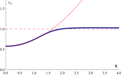
Figure 1: Sound dispersion $c_{s}=c_{s}(\textswab{q})$ in ${\cal N}=4$ SYM plasma. The dark (blue) curve shows the sound speed dependence on wavevector, $c_{s}(\textswab{q})=\mbox{Re}\,\textswab{w}/\textswab{q}$, with $c_{s}(0)=1/\sqrt{3}$ (this plot is based on numerical data first obtained in [31]). The light (red) curve corresponds to analytic approximation derived from Eq. (76) and valid for sufficiently small $\textswab{q}$.

4.4 Bjorken flow

In order to determine $\lambda_{1}$, we match Eq. (55) with the solution found by Heller and Janik [17] given by

$$\varepsilon(\tau)=\frac{N_{c}^{2}}{2\pi^{2}}\left[\tau^{-4/3}-2\eta_{0}\tau^{-2}+\tau^{-8/3}\left(\frac{10}{3}\eta_{0}^{2}+\frac{6\ln 2-17}{36\sqrt{3}}\right)\right],\quad\textrm{with}\quad\eta_{0}=\frac{1}{\sqrt{2}\,3^{3/4}}\,.$$ (78)

Matching by using $C=N_{c}^{2}/(2\pi^{2})$, and $\tau_{\Pi}=(2-\ln 2)/(2\pi T)$ from Eq. (77), together with $\varepsilon=3\pi^{2}N_{c}^{2}T^{4}/8$ and Eq. (54) gives

$$\lambda_{1}=\frac{\eta}{2\pi T}.$$ (79)

Note that Heller and Janik [17] found a different value for $\tau_{\Pi}$ since they matched to the Israel-Stewart equations for hydrodynamics, and not the more general (nonlinear) equation (33).

5 Kinetic theory

Our analysis should be valid not only for the strongly coupled ${\cal N}=4$ SYM theory, but also for all theories with conformal symmetry. In particular, it should be valid also for weakly coupled CFT like the SYM theory at small ’t Hooft coupling, or QCD at sufficiently large $N_{f}$ at the Banks-Zaks fixed point [32]. In these cases, one expects that it is possible to understand and compute the second-order transport coefficient from kinetic theory. We set $d=4$ in this Section.

5.1 Setup

Since we are to discuss conformal transformations, our starting point is the classical Boltzmann equation in curved rather than flat space-time [33, 34],

$$\left[p^{\mu}\frac{\partial}{\partial x^{\mu}}-\Gamma^{\lambda}_{\mu\nu}p^{\mu}p^{\nu}\frac{\partial}{\partial p^{\lambda}}\right]f(p,x)=-{\mathcal{C}}[f],$$ (80)

where $f(p,x)$ is the one-particle distribution function, $p^{\mu}$ is the particle momentum, $\Gamma^{\lambda}_{\mu\nu}$ are the Christoffel symbols and ${\mathcal{C}}$ is the collision integral. One can easily show that conformal transformations are a symmetry of the Boltzmann equation if particles are massless ($p^{2}\equiv p^{\mu}p_{\mu}=0$) and the collision integral transforms as ${\mathcal{C}}[\bar{f}]\rightarrow e^{2\omega(x)}{\mathcal{C}}[f]$.

Hydrodynamic equations are obtained by taking moments with respect to the particle momentum $p^{\mu}$ of Eq. (80). More precisely, acting with $\int d\chi\equiv\int d^{4}p\delta(-p^{2})\theta(p^{0})$, where $\theta$ is the step-function, on Eq. (80) one obtains

$$\int d\chi\sqrt{-g}\left[p^{\mu}\frac{\partial}{\partial x^{\mu}}-\Gamma^{\lambda}_{\mu\nu}p^{\mu}p^{\nu}\frac{\partial}{\partial p^{\lambda}}\right]f(p,x)=-\int d\chi\sqrt{-g}{\mathcal{C}}[f],$$ (81)

which upon partial integration leads [34] to

$$\nabla_{\mu}\int d\chi p^{\mu}\sqrt{-g}f(p,x)=-\int d\chi\sqrt{-g}{\mathcal{C}}[f].$$ (82)

We recall here that $\nabla_{\mu}$ is the (geometric) covariant derivative. In theories with conserved charges or if only elastic collisions are considered, $\int d\chi{\mathcal{C}}[f]=0$ and Eq. (82) becomes the conservation of the particle current in theories with conserved charges. Conservation of the energy-momentum tensor

$$T^{\mu\nu}\equiv\int d\chi p^{\mu}p^{\nu}\sqrt{-g}f(p,x)$$ (83)

follows from Eq. (80) upon action of $\int d\chi p^{\nu}$ and the requirement $\int d\chi\sqrt{-g}p^{\nu}{\mathcal{C}}[f]=0$,

$$\nabla_{\mu}T^{\mu\nu}=0.$$ (84)

Acting with $\int d\chi p^{\nu}p^{\lambda}$ on Eq. (80) gives the first equation with non-trivial contribution from the collision integral [36],

$$\nabla_{\mu}X^{\mu\nu\lambda}=I^{\nu\lambda},$$ (85)

where

$$X^{\mu\nu\lambda} \equiv \int d\chi p^{\mu}p^{\nu}p^{\lambda}\sqrt{-g}f(p,x)\,,$$ (86)

$$I^{\nu\lambda} \equiv -\int d\chi p^{\nu}p^{\lambda}\sqrt{-g}{\mathcal{C}}[f].$$ (87)

Similarly, an infinity of higher moment equations of the form

$$\nabla_{\mu}X^{\mu\nu_{1}\nu_{2}\nu_{3}\ldots}=I^{\nu_{1}\nu_{2}\nu_{3}\ldots}$$ (88)

also follow from Eq. (80).

Splitting the out-of-equilibrium particle distribution function into an equilibrium and non-equilibrium part

$$f(p,x)=f_{\rm eq}(p,x)\left(1+\delta f(p,x)\right),$$ (89)

one defines an equilibrium energy-momentum tensor

$$T^{\mu\nu}_{\rm eq}=T^{\mu\nu}\equiv\int d\chi p^{\mu}p^{\nu}\sqrt{-g}f_{\rm eq}(p,x)\,,$$ (90)

and a non-equilibrium component $\Pi^{\mu\nu}=T^{\mu\nu}-T^{\mu\nu}_{\rm eq}$, which by construction is both symmetric and traceless. We shall assume that the equilibrium distribution function $f_{\rm eq}(p,x)=f_{\rm eq}(-u(x)\cdot p/T(x))$ depends on local temperature and velocity $T,u_{\mu}$, which are defined such that the equilibrium distribution has the same energy and momentum density as $f$ in the rest frame defined by $u_{\mu}$,

$$\int d\chi\sqrt{-g}p^{\mu}(u_{\nu}p^{\nu})\left(f-f_{\rm eq}\right)=0.$$ (91)

This implies that $u_{\mu}\Pi^{\mu\nu}=0$.

5.2 Moment approximation

While the full hierachy of moment equations should correspond to the original Boltzmann equation, it is too complicated to be treated exactly. However, an approximate evolution equation for systems not too far from equilibrium may be constructed. The approximation is similar to the Grad’s 14-moment method [37].

We decompose $\delta f$ into spherical harmonics,

$$\delta f=\sum_{l=0}^{\infty}f^{(l)}_{\mu_{1}\ldots\mu_{l}}(\xi)p^{\mu_{1}}\ldots p^{\mu_{l}},\quad\xi=-\frac{u\cdot p}{T},$$ (92)

where $f^{(l)}_{\mu_{1}\ldots\mu_{l}}(\xi)$ are fully symmetric, orthogonal to $u^{\mu}$, and traceless over any pair of indices. By construction, the $l=0,1$ parts satisfy the constraints Eq. (91). The approximation is now specified by the following assumptions (c.f. [38]):

• the system is sufficiently close to equilibrium that the collision term is linear in $\delta f$

• all contributions $l>2$ are subdominant

• for $l\leq 2$ and expanding in some basis, all $\xi$ dependent terms are subdominant.

This implies that

$$\delta f(p,x)\sim T^{-6}p^{\mu}p^{\nu}\Pi_{\mu\nu}+{\mathcal{O}}(\Pi^{2}),$$ (93)

and

$$I^{<\nu\lambda>}\sim T^{2}(x)\Pi^{<\nu\lambda>}(x)+{\mathcal{O}}(\Pi^{2}),$$ (94)

where subdominant terms have been labelled as ${\mathcal{O}}(\Pi^{2})$. It would be interesting to use numerical techniques such as in Ref.[39, 40] to test the correctness of Eq. (93).

Splitting $X^{\mu\nu\lambda}$ into an equilibrium and non-equilibrium part, one finds

$$X^{\mu\nu\lambda}_{\rm eq}=\int d\chi p^{\mu}p^{\nu}p^{\lambda}\sqrt{-g}f_{\rm eq}(p,x)\sim T^{5}\left[\ u^{\mu}u^{\nu}u^{\lambda}+{\rm const}\times\left(\Delta^{\mu\nu}u^{\lambda}+perm.\right)\right],$$ (95)

where $perm.$ denotes all non-trivial permutations of indices, and

$$X^{\mu\nu\lambda}-X^{\mu\nu\lambda}_{\rm eq}\sim T\Pi^{(\mu\nu}u^{\lambda)},$$ (96)

where $(\mu_{1}\mu_{2}\ldots\mu_{n})$ denotes symmetrization with respect to the indices $\mu_{1},\mu_{2},\ldots,\mu_{n}$. Projection $<>$ on the moment equation (85) thus gives

$$\Pi^{\nu\lambda}+\tau_{\Pi}\left[\Pi^{\nu\lambda}D{\rm ln}T+\Delta^{\nu}_{\alpha}\Delta^{\lambda}_{\beta}D\Pi^{\alpha\beta}+\Pi^{\nu\lambda}\nabla_{\mu}u^{\mu}+2\Pi^{\mu<\nu}\nabla_{\mu}u^{\lambda>}\right]=-\eta\sigma^{\nu\lambda}+{\mathcal{O}}(\Pi^{2}),$$ (97)

where the proportionality constants have been denoted by $\eta$ and $\tau_{\Pi}$, respectively (the ratio of these can be calculated when specifying $f_{\rm eq}$, c.f.[19]). Introducing the completely symmetric tensor

$$\theta_{\mu\rho}=\frac{1}{2}\Delta^{\alpha}_{\mu}\Delta^{\beta}_{\rho}\left(\nabla_{\alpha}u_{\beta}+\nabla_{\beta}u_{\alpha}\right)$$ (98)

one can decompose

$$\Pi^{\mu<\nu}\nabla_{\mu}u^{\lambda>}=-\Pi^{\alpha(\nu}\Omega^{\lambda)}_{\ \alpha}+\Pi^{\alpha(\nu}\theta_{\alpha}^{\ \lambda)}-\frac{1}{3}\Pi^{\alpha\beta}\Delta^{\nu\lambda}\theta_{\alpha\beta}.$$ (99)

Rewriting

$$\theta_{\mu\rho}=\nabla^{\perp}_{<\mu}u_{\rho>}+\frac{1}{3}\Delta_{\mu\rho}\nabla^{\perp}_{\gamma}u^{\gamma}$$ (100)

such that

$$\Pi^{\mu<\nu}\nabla_{\mu}u^{\lambda>}=-\Pi^{\alpha(\nu}\Omega^{\lambda)}_{\ \alpha}+\frac{1}{3}\Pi^{\nu\lambda}\nabla_{\gamma}u^{\gamma}-\frac{\Pi^{\alpha<\nu}\Pi^{\lambda>}_{\alpha}}{2\eta}+{\mathcal{O}}(\Pi^{3}),$$ (101)

we find

$$\Pi^{\nu\lambda}=-\eta\sigma^{\nu\lambda}-\tau_{\Pi}\left[D\Pi^{<\nu\lambda>}+\frac{4}{3}\Pi^{\nu\lambda}(\nabla\cdot u)\right]+2\tau_{\Pi}\Pi^{\alpha(\nu}\Omega^{\lambda)}_{\ \alpha}+\frac{\lambda_{1}}{\eta^{2}}\Pi^{\alpha<\nu}\Pi^{\lambda>}_{\alpha}+{\mathcal{O}}(\Pi^{3})\,,$$ (102)

where $D\ln T=-\frac{1}{3}(\nabla\cdot u)+{\mathcal{O}}(\Pi^{2})$ has been used.

Eq. (102), which was derived from kinetic theory here, corresponds to the more general Eq. (33) with $\lambda_{2}=-2\tau_{\Pi}\eta$ and $\lambda_{3}=\kappa=0$. Note that $\lambda_{1}$ contains a contribution from Eq. (101) as well as from the collision integral Eq. (94) (see below). What is commonly referred to as Israel-Stewart theory amounts to setting $\lambda_{1}=0$. Most of the time, also the terms involving $\nabla\cdot u$ and the vorticity $\Omega^{\mu\nu}$ are dropped. However, note that simply dropping terms involving $\nabla\cdot u$ ruins the conformal symmetry of the equation, and thus the resulting equation cannot be the correct hydrodynamic description of the system dynamics beyond leading order.

5.3 The structure of the collision integral

In this subsection we study the structure of the collision integral Eq. (94) for a simplified model where ${\mathcal{C}}=(u\cdot p)\frac{f-f_{\rm eq}}{\tau_{\Pi}}$. We will use a gradient expansion similar to the Chapman-Enskog method (c.f. [41]).

Let us decompose $f$ into

$$f=f_{\rm eq}(-u\cdot p/T)\left(1+f_{1}+f_{2}+\ldots\right),$$ (103)

where $f_{1},f_{2}$ represent terms of first and second order in gradients, respectively. Solving Eq. (80) iteratively in gradients we find

$$f_{1} = \frac{\tau_{\Pi}}{p\cdot u}\frac{f_{\rm eq}^{\prime}}{f_{\rm eq}}p^{\mu}p^{\alpha}\nabla_{\mu}\frac{u_{\alpha}}{T}\,,$$

$$f_{2} = \frac{\tau_{\Pi}^{2}}{(p\cdot u)^{3}}\frac{(p\cdot u)f_{\rm eq}^{\prime\prime}+Tf_{\rm eq}^{\prime}}{f_{\rm eq}}p^{\mu}p^{\nu}p^{\alpha}p^{\beta}\nabla_{\mu}\left(\frac{u_{\alpha}}{T}\right)\nabla_{\nu}\left(\frac{u_{\beta}}{T}\right)$$ (104)

$$-\frac{\tau_{\Pi}^{2}}{(p\cdot u)^{2}}\frac{f_{\rm eq}^{\prime}}{f_{\rm eq}}p^{\mu}p^{\nu}p^{\alpha}\nabla_{\nu}\nabla_{\mu}\frac{u_{\alpha}}{T}+\frac{2\tau_{\Pi}^{2}}{(p\cdot u)^{2}}\frac{f_{\rm eq}^{\prime}}{f_{\rm eq}}p^{\mu}p^{\nu}p^{\alpha}\nabla_{\mu}\left(\frac{u_{\alpha}}{T}\right)\nabla_{\nu}\ln T\,.$$

From Eq. (94) and conformal symmetry, to second order in gradients the collision integral $I^{<\gamma\delta>}$ can contain terms $\sigma^{<\gamma}_{\lambda}\sigma^{\delta>\lambda}$ and $D\sigma^{<\gamma\lambda>}+\frac{1}{3}\sigma^{\gamma\lambda}(\nabla\cdot u)$ but (in particular) not $\Omega^{\gamma\delta}$ or $R^{\gamma\delta}$ since these terms would involve anti-symmetrization of indices which is not allowed by Eq. (104).

This indicates that the terms involving $\kappa,\lambda_{3}$ in Eq. (33) are not contained in the Boltzmann equation. The Boltzmann equation is only an approximation of the underlying quantum field theory, so it is possible that these terms – which are second order in gradients – have been lost in this coarse-graining process. It may be possible to compute the coefficients of these terms for QCD in the weak-coupling regime by going beyond the lowest order gradient expansion given in [42].

6 Analysis of the Müller-Israel-Stewart theory

6.1 Causality in first order hydrodynamics

It is instructive to compare the second-order conformal hydrodynamics to the Müller-Israel-Stewart theory. Müller [7] and independently later Israel and Stewart [8, 9, 10], considered how to extend the 1st order hydrodynamics. Their primary motivation was to eliminate the apparent relativistic acausality of the 1st order hydrodynamic equations. Formally, the acausality is the result of the fact that the 1st order hydrodynamic equations are not hyperbolic [43, 10, 44]. The problem is most clearly seen by considering the linearized equation for a diffusive mode (e.g., shear stress or charge diffusion), which is first order in temporal but second in spatial derivatives. A discontinuity in initial conditions for such a mode propagates at infinite speed. In other words, the influence of an initial condition at a point in space is instanteneously felt by any other point.

It should be clear, however, as emphasized, e.g., by Geroch [45, 46] and others [47] that the modes which defy causality are those which are not supposed to be described by hydrodynamics (i.e., microscopically short wavelengths, which is clear when one thinks about discontinuities). Nevertheless, for numerical simulations of relativistic hydrodynamic systems such superluminal propagation is a nuisance because in such simulations one extrapolates hydrodynamic equations to the microscopic scale, even though the modes, or the configurations, which are being studied are hydrodynamic. For example, superluminal propagation makes posing initial value problem difficult: even if the initial hypersurface is space-like, the initial values at different points can influence each other and an attempt to specify them independently leads to unacceptable singular solutions [48, 47].

Since the problem lies in the domain where the theory is not applicable, one can safely modify the theory in this domain, without disturbing physical predictions. This is the essence of the solution which Müller and Israel proposed by extending the set of variables. The resulting system of equations is hyperbolic. Here we shall write down explicitly the system of equations of Israel and Stewart, restricting to the case of conformally invariant system without a conserved charge that we study in this paper.

6.2 Hydrodynamic variables and second order hydrodynamics

As we have already emphasized in Section 2.2 the hydrodynamics should be viewed as a controllable expansion in gradients of the hydrodynamic variables. The choice of the variables, or fields, can be aided by applying the requirement that a linearized system of equations has solutions whose frequency vanishes in the hydrodynamic limit, i.e., when the wave vector $\bm{k}$ vanishes. We call such linearized modes the hydrodynamic modes. Fluctuations of conserved densities are automatically hydrodynamic because their equations are conservation laws and constant fields ($\omega=0$, $\bm{k}=0$) are trivial solutions of them.

Hence, for a system without conserved charges the set of hydrodynamic variables consists of the densitites of energy and momentum, represented by 4 independent covariant variables $\varepsilon$ and $u^{\mu}$ ($u{\cdot}u=-1$). All other quantities in hydrodynamic description are instantaneous functions of these variables and their derivatives, such as, e.g., $\Pi^{\mu\nu}$ (Section 2.2).

How should one extend 1st order hydrodynamics to higher derivatives? The systematic way, as we argued in Section 2.2 and 3, is to continue the expansion (16) and add all possible terms of the second order in derivatives, as we did in Eq. (32).

Instead, Müller, Israel and Stewart take a more phenomenological point of view. They consider $\Pi^{\mu\nu}$ – the viscous part of the the momentum flow – as a set of independent additional variables. The equations for these variables are not given by any exact conservation laws, but by phenomenological expansions in the set of independent variables, which now includes also $\Pi^{\mu\nu}$:

$$\tau_{\Pi}D\Pi^{\mu\nu}=-\Pi^{\mu\nu}-\eta\sigma^{\mu\nu}\,.$$ (105)

The first term in Eq. (105) has a simple intuitive meaning: in the absence of velocity gradients ($\sigma^{\mu\nu}=0$) the viscous momentum flows $\Pi^{\mu\nu}$ do not vanish instanteneously (as in Eq. (16)), but relax to zero on a microscopic but finite timescale $\tau_{\Pi}$. The 5 equations (105) together with 4 conservation laws $\nabla_{\mu}T^{\mu\nu}=0$ form the system of Müller-Israel-Stewart equations for 9 variables: $\varepsilon$, $u^{\mu}$ and $\Pi^{\mu\nu}$. (For a non-conformal system with a conserved charge this number becomes 14.)

In the phenomenological laws in Eq. (105) one usually considers only terms linear in the variables $\Pi^{\mu\nu}$ and $u^{\mu}$. There is a priory no reason to neglect nonlinear terms. By comparing Eq. (105) with Eq. (33) we see that the conformal invariance requires presence of terms proportional to $\Pi^{\mu\nu}(\nabla{\cdot}u)$, which are non-linear, but contain the same number of derivatives. These terms are beyond the standard linear Israel-Stewart phenomenological theory. In addition, bilinear terms proportional to $\lambda_{i}$ are also allowed to the same order in derivatives. Such terms are relevant for simulations of the strongly coupled quark-gluon plasma in heavy ion collisions.

The term proportional to $\kappa$, which vanishes in flat space, has not been considered by Israel and Stewart but, as we have seen, is necessary to determine the correlation functions of stress-energy tensor.

Note that in this scheme both $\Pi^{\mu\nu}$ and $\sigma^{\mu\nu}$ are of the same, i.e., first order in the expansion around equilibrium. The term $D\Pi^{\mu\nu}$ contains one more derivative compared to $\Pi^{\mu\nu}$ and is thus of the second order. Without loss of precision, to second order, one can trade $D\Pi^{\mu\nu}$ for $-D(\eta\sigma^{\mu\nu})$ or vice versa. Similar substitutions can be made in other second-order terms we found, as we did when going from Eq. (32) to Eq. (33). Therefore, within their precision, equations of Israel-Stewart (105) (or, in general nonlinear case, Eq. (33)) give the same result as the systematic expansion in derivatives.

6.3 Causality and the domain of applicability

The attractive feature of introducing new variables is that the resulting equations are now first order in derivatives and, most importantly, they are hyperbolic. This means that discontinuities propagate with finite velocities even in the shear channel. For the shear channel this velocity (i.e., the characteristic velocity [43, 49, 44]) can be easily obtained from the dispersion relation (48) by taking $k\to\infty$:

$$v_{\rm disc}=\sqrt{\frac{\eta}{\tau_{\Pi}\,(\varepsilon+P)}}.$$ (106)

Although the Israel-Stewart system of equations (105) or our equations (33), have attractive features from the point of view of the mathematical formulation, and are especially suitable to, e.g., numerical simulations, care should be taken attributing physical significance to this fact. The domain of applicability of these equations is still the hydrodynamic domain: $\omega$, $k$ must be small compared to microscopic scales. The second order hydrodynamic equations increase the precision compared with the first order equations, but only if we stay within the hydrodynamic domain.

In practice, it is convenient to use equations which are mathematically well-behaved even where they lose physical significance. However, care should be taken when examining the solutions by always considering only their features in hydrodynamic domain – slow and long-wavelength modes. In particular, the velocity in Eq. (106) does not correspond to any physical propagation. Similarly, the superluminal propagation which one recovers according to Eq. (106) in the first order theory when $\tau_{\Pi}\to 0$ is the result of extrapolating the theory outside the hydrodynamic domain.

Nevertheless it is worthwhile to note that, with the value of $\tau_{\Pi}$ in strongly coupled ${\cal N}=4$ SYM that we find in Eq. (66), the characteristic velocity (106) equals $1/\sqrt{2(2-\log 2)}=0.6\ldots$, i.e., less than the velocity of light. Therefore, the system of second order equations we wrote down can be used in, e.g., numerical simulations without additional modifications often needed to ensure relativistic causality and prevent occurence of singular solutions.

6.4 Entropy and the second law of thermodynamics

Let us consider the question of how the second law of thermodynamics is obeyed by the second order hydrodynamics. For that purpose take the projection of the energy-momentum conservation equation on $u^{\nu}$:

$$0=-u_{\nu}\nabla_{\mu}T^{\mu\nu}=D\varepsilon+(\varepsilon+P)\nabla{\cdot}u+\Pi^{\mu\nu}\nabla_{\mu}u_{\nu},$$ (107)

where we used definition Eq. (22), $u{\cdot}u=-1$ and $u_{\nu}\Pi^{\mu\nu}=0$. For a system without a conserved charge, the thermodynamic entropy density $s$ is a function of the energy density such that $ds=d\varepsilon/T$, and it also obeys $sT=\varepsilon+P$. Thus, Eq. (107) can be writen as

$$T\nabla_{\mu}(su^{\mu})=-\Pi_{\mu\nu}\nabla^{\mu}u^{\nu}.$$ (108)

Since $s$ is the entropy in the local rest frame, equation (108) expresses, in a covariant form, the rate of entropy production in the local rest frame.

For a conformal system the tensor $\Pi_{\mu\nu}$ is traceless and one can replace $\nabla^{\mu}u^{\nu}$ on the r.h.s. of Eq. (108) with $\sigma^{\mu\nu}/2$. Using the first order hydrodynamic relation (23) one then finds

$$\nabla_{\mu}(su^{\mu})=\frac{\eta}{2T}\,\sigma_{\mu\nu}\sigma^{\mu\nu}+\textrm{(3rd order terms)}.$$ (109)

Thus, if $\eta>0$, the entropy increases, provided the 3rd order terms on the r.h.s. of Eq. (109) are negligible compared to the 2nd order term written out. This is always true within the domain of validity of hydrodynamics.

Müller and Israel observed [7, 8] that the third order terms in Eq. (109) in their theory can be written as the divergence of a current. Indeed, even a complete, conformally covariant, term proportional to $\tau_{\Pi}$ in Eq. (33) can be written in such a way. Solving (33) for $\sigma^{\mu\nu}$ and substituting into Eq. (108) we find

$$\nabla_{\mu}(su^{\mu}) = \frac{1}{2\eta T}\,\Pi_{\mu\nu}\Pi^{\mu\nu}+\nabla_{\mu}\left(\frac{\tau_{\Pi}}{4\eta T}\Pi_{\alpha\beta}\Pi^{\alpha\beta}u^{\mu}\right)$$ (110)

$$-\frac{1}{2\eta T}\,\Pi_{\mu\nu}\left(\kappa{\cal O}_{2}^{\mu\nu}+{\lambda_{1}}{\cal O}_{3}^{\mu\nu}+{\lambda_{2}}{\cal O}_{4}^{\mu\nu}+{\lambda_{3}}{\cal O}_{5}^{\mu\nu}\right)+\ldots\,,$$

where we used $\tau_{\Pi}/\eta={\rm const}{\cdot}T^{-d}$ and the lowest order relation $D\ln T=-(d-1)\nabla{\cdot}u$. The ellipsis in Eq. (110) denotes 4-th order corrections. Therefore, defining non-equillibrium entropy as

$$s_{\rm noneq}=s-\frac{\tau_{\Pi}}{4\eta T}\Pi_{\alpha\beta}\Pi^{\alpha\beta}$$ (111)

one can cancel the 3rd order term proportional to $\tau_{\Pi}$ in $\nabla_{\mu}(s_{\rm noneq}u^{\mu})$. The correction to the equillibrium entropy in Eq. (111) has an intuititive meaning – a non-homogeneous state of the system, in which $\Pi_{\mu\nu}\neq 0$, has smaller entropy than the equilibrium state.

The remaining terms, such as e.g., $\kappa\Pi_{\mu\nu}{\cal O}_{2}^{\mu\nu}/(\eta T)$, do not appear to be total derivatives. They are also not positive definite. However, this fact cannot be used to conclude that, e.g., $\kappa$ must be zero. Our explicit AdS/CFT calculation shows that $\kappa\neq 0$. As we discussed above, the 3rd order terms in Eq. (109) do not violate the second law of thermodynamics if we stay within the domain of applicability of hydrodynamics. In this domain the 3rd order terms must be small compared to the second order term on the r.h.s. of Eq. (109), which is positive definite.

Further detailed discussions on the issue of the local entropy current can be found in [50, 51].

6.5 Additional non-hydrodynamic modes

Another interesting consequence of introducing more variables, à la Müller-Israel-Stewart, is that the number of modes, or branches of the dispersion relation $\omega(\bm{k})$ increases, as we have seen in Sections 3.3 and 3.4. As should be expected, the additional poles are not hydrodynamic: those frequencies $\omega(\bm{k})$ do not vanish as $\bm{k}\to 0$, but remain on the order of the microscopic scale. It should be clear from the discussion above that the position of these poles need not be predicted correctly by the second-order theory – they lie outside of the regime of its validity.

In fact, now with the knowledge of the position of Green’s function singularities in ${\cal N}=4$ SYM at strong coupling [31] we can say that there are infinitely many such poles. They are given by the solutions of equations such as (67) or (71). Only the lowest branch $\omega(\bm{k})$ can be matched by hydrodynamic theory. To describe correctly the full Green’s function one needs to introduce infinitely many degrees of freedom – to describe infinitely many poles. Any theory of finite number of degrees of freedom is a truncation. This truncation is controllable only for the hydrodynamic variables, which describe the poles with frequencies vanishing as $\bm{k}\to 0$. The controlling parameter is the ratio of these frequencies to a microscopic scale, i.e., $T$ in the conformal theory, and the precision can be, in principle, increased by increasing the order of the expansion in this parameter.

Conceptually, let us imagine that we did succeed in writing the infinite set of extended hydrodynamic equations for infinitely many variables, mentioned in the previous paragraph. It is easy to realize that in a theory with gravity dual this set will be mathematically equivalent (in the linear regime) to differential equations (67) or (71). The set of infinitely many 4-dimensional fields is represented by a 5-dimensional field in these equations.

7 Conclusion

We have determined the most general form of relativistic viscous hydrodynamics of a conformal fluid (with no conserved charges) to second order in gradients. We find that conformal invariance reduces the number of allowed terms relative to more general, non-conformal, hydrodynamics. As already known, at first order in gradients only one kinetic coefficient, the shear viscosity $\eta$, enters the equations. At second order we find five allowed terms with coefficients $\tau_{\Pi}$ (customarily referred to as relaxation time), $\kappa$, $\lambda_{1}$, $\lambda_{2}$ and $\lambda_{3}$.

The general viscous hydrodynamic equations we obtained can be matched to AdS/CFT calculations in strongly coupled ${\cal N}=4$ supersymmetric Yang-Mills theory, and for this theory we thus determined three of the five second-order coefficients: $\tau_{\Pi}$, $\kappa$ and $\lambda_{1}$. We also find that for a weakly coupled conformal plasma describable by the Boltzmann equation, two of the coefficients vanish. However, at least one of these coefficients, i.e., $\kappa$, is not zero for strongly coupled ${\cal N}=4$ super Yang-Mills theory. It would be interesting to understand how this coefficient emerges as the approximation of the Boltzmann equation breaks down at large coupling.

We emphasized the already known fact that the equations of the Müller-Israel-Stewart theory, despite their appearance, are only applicable in the hydrodynamic regime, where their predictions coincide with those of the second-order gradient expansion. We also pointed out that variants of the Müller-Israel-Stewart theory used in numerical simulations of relativistic plasmas frequently miss terms which are not only allowed, but also required for conformally invariant theories. If the quark-gluon plasma is approximately conformal, then the second-order hydrodynamic equation found in this paper should be used instead. One may hope that the values of the kinetic coefficients $\tau_{\Pi}$ and $\lambda_{1}$, found in ${\cal N}=4$ SYM theory, may serve as crude estimates for their values in the strongly coupled regime of the quark-gluon plasma.

Appendix A Perturbative solutions of the shear and the sound mode equations

The shear mode

The functions $G_{i}(u)$ entering the perturbative solution (68) of the equation (67) are

$$G_{0}(u)=Cu\,,\qquad G_{1}(u)=iC\left(u-1+\frac{u}{2}\ln{\frac{u+1}{2}}\right)\,,\qquad G_{2}(u)=\frac{C(1-u)}{2}\,,$$ (112)

$$G_{3}(u) = -\frac{C}{48}\Biggl{(}6\pi^{2}u-24(u+1)\ln{2}-i12\pi u\ln 2-6u\ln^{2}2+18u\ln^{2}(u-1)$$

$$+ 24(u+1)\ln(u+1)+12u\ln 2\ln{\frac{1+u}{1-u}}-12u\ln(1+u)\ln{\frac{1+u}{1-u}}+6u\ln^{2}\frac{1+u}{1-u}$$

$$- 24u\mbox{Li}_{2}\left(\frac{1-u}{2}\right)+12u\ln(u-1)\Biggl{(}\ln 2-2\ln(1-u)-i\pi\Biggr{)}\Biggr{)}\,,$$

$$G_{4}(u) = \frac{C}{16}\Biggl{(}-4\pi u-4i(1+3u)\ln 2+4i\ln(1+u)+16iu\ln{\frac{1+u}{u}}+2iu\ln(u-1)\left(\ln{\frac{1+u}{1-u}}\right)$$

$$- 4iu\ln{\frac{1+u}{1-u}}+2\pi u\ln{\frac{1+u}{1-u}}-2iu\ln(1+u)\ln{\frac{1+u}{1-u}}+2iu\ln^{2}\frac{1+u}{1-u}-4iu\ln(u-1)\Biggr{)}\,,$$

$$G_{5}(u) = \frac{C}{4}\Biggl{(}1-u-2u\ln{\frac{1+u}{2u}}\Biggr{)}\,,$$ (113)

where $C$ is a constant, $\mbox{Li}_{2}(z)$ is a polylogarithm.

An alternative way to obtain the dispersion relation (69) is the following: the functions $G_{i}(u),i=0,1,..5$ satisfy the inhomogeneous differential equations

$$(1-u^{2})G_{i}^{{}^{\prime\prime}}-2uG_{i}^{{}^{\prime}}+2G_{i}=F_{i}(u)~{},$$ (114)

with $F_{0}=0,F_{1}=-i(1+u)G_{0}^{{}^{\prime}}-i/2G_{0},etc.$ The homogeneous part of (114) is the Legendre differental equation with the Legendre functions $P_{1}(u)=u$ and $Q_{1}(u)=\frac{u}{2}\ln{\frac{1+u}{1-u}}-1$ as solutions. Therefore $G_{0}=Cu$, and for $i\geq 1$

$$G_{i}(u)=P_{1}(u)\int_{u}^{1}~{}Q_{1}(u^{\prime})F_{i}(u^{\prime})du^{\prime}-Q_{1}(u)\int_{u}^{1}~{}P_{1}(u^{\prime})F_{i}(u^{\prime})du^{\prime}~{},$$ (115)

regular at $u=1$. Finally, the values at $u=0$ are obtained by

$$G_{i}(u=0)=\int_{0}^{1}~{}uF_{i}(u)du~{},$$ (116)

i.e. $G_{0}(0)=0,G_{1}(0)=-iC,$ and

$$G_{2}(0) = \int_{0}^{1}G_{0}(u)du=C/2,$$

$$G_{3}(0) = \frac{C}{4}\int_{0}^{1}~{}u\left[(2+3u)\ln{\frac{1+u}{2}}+7u-\frac{2}{1+u}\right]du=C\frac{\ln 2}{2}\,,$$ (117)

etc., and hence we find Eq. (69).

The sound mode

The functions $X_{i}(u)$ of the perturbative solution (74) of the equation (73) are

$$X_{0}(u)=\frac{(\textswab{q}^{2}+\textswab{q}^{2}u^{2}-3\textswab{w}^{2})C}{4\textswab{q}^{2}}\,,\qquad X_{1}(u)=-\frac{iC\textswab{w}f(u)}{2}\,,$$ (118)

$$X_{2}(u) = \frac{C}{48\textswab{q}^{2}}\Biggl{[}2\textswab{q}^{2}\Biggl{(}8-8u-i\pi(1+u^{2})-(1+u^{2})\,2\ln{2}\Biggr{)}$$ (119)

$$+ 3\textswab{w}^{4}\Biggl{(}\pi^{2}-6i\pi-\ln{8}\left(\ln{8}-4\right)\Biggr{)}$$

$$+ \textswab{q}^{2}\textswab{w}^{2}\Biggl{(}6i\pi(2+u^{2})-\pi^{2}(1+u^{2})-24\,(u^{2}-u+\ln{2})+\ln{8}\left(\ln{8}+u^{2}(4+\ln{8})\right)\Biggr{)}$$

$$- 2(\textswab{q}^{2}-3\textswab{w}^{2})(\textswab{q}^{2}(1+u^{2})-3\textswab{w}^{2})\left(-i\pi+\log{(1-u)}\right)$$

$$+ 4\Biggl{(}\textswab{q}^{4}(1+u^{2})+9\textswab{w}^{4}(\ln{2}-1)-3\textswab{w}^{2}\textswab{q}^{2}\left(\ln{2}-2+u^{2}(\ln{2}+1)\right)\Biggr{)}\ln{(1+u)}$$

$$+ 3\textswab{w}^{2}\left(\textswab{q}^{2}(1+u^{2})-3\textswab{w}^{2}\right)\ln^{2}(1+u)$$

$$+ 2\left(\textswab{q}^{2}(1+u^{2})-3\textswab{w}^{2}\right)\left(\textswab{q}^{2}-3\textswab{w}^{2}(1+\ln{2})+3\textswab{w}^{2}\ln{(1+u)}\right)\ln{(1-u)}$$

$$+ 6\textswab{w}^{2}\left(\textswab{q}^{2}(1+u^{2})-3\textswab{w}^{2}\right)\mbox{Li}_{2}\left(\frac{1+u}{2}\right)\Biggr{]}\,.$$

References

- [1] L.D. Landau and E.M. Lifshitz, Fluid Mechanics, 2nd ed., Pergamon Press 1987.
- [2] L.P. Kadanoff and P.C. Martin, Hydrodynamic equations and correlation functions, Ann. Phys. (NY) 24 (1963) 419.
- [3] J. Maldacena, The large N limit of superconformal field theories and supergravity, Adv. Theor. Math. Phys. 2 (1998) 231 [Int. J. Theor. Phys. 38 (1999) 1113] [hep-th/9711200].
- [4] P. Kovtun and L. G. Yaffe, Hydrodynamic fluctuations, long-time tails, and supersymmetry, Phys. Rev. D 68 (2003) 025007 [hep-th/0303010].
- [5] P. C. Hohenberg and B. I. Halperin, Theory of dynamic critical phenomena, Rev. Mod. Phys. 49 (1977) 435.
- [6] D. Burnett, The distribution of molecular velocities and the mean motion in a non-uniform gas, Proc. London Math. Soc. 40 (1936) 382.
- [7] I. Müller, Zum Paradoxon der Wärmeleitungstheorie, Z. Phys. 198 (1967) 329.
- [8] W. Israel, Nonstationary irreversible thermodynamics: A causal relativistic theory, Ann. Phys. (NY) 100 (1976) 310.
- [9] W. Israel and J. M. Stewart, Thermodynamics of nonstationary and transient effects in a relativistic gas, Phys. Lett. A 58 (1976) 213.
- [10] W. Israel and J. M. Stewart, Transient relativistic thermodynamics and kinetic theory, Ann. Phys. (NY) 118 (1979) 341.
-
[11]
J. S. Schwinger,
Brownian motion of a quantum oscillator,
J. Math. Phys. 2 (1961) 407;
L. V. Keldysh, Diagram technique for nonequilibrium processes, Zh. Eksp. Teor. Fiz. 47 (1964) 1515 [Sov. Phys. JETP 20 (1965) 1018];
P. M. Bakshi and K. T. Mahanthappa, Expectation value formalism in quantum field theory. 1, J. Math. Phys. 4 (1963) 1; Expectation value formalism in quantum field theory. 2, J. Math. Phys. 4 (1963) 12; - [12] N. D. Birrell and P. C. W. Davies, Quantum Fields in Curved Space, Cambridge University Press 1982.
- [13] M. J. Duff, Twenty years of the Weyl anomaly, Class. and Quant. Grav. 11 (1994) 1387 [hep-th/9308075].
- [14] O. Aharony, S. S. Gubser, J. Maldacena, H. Ooguri and Y. Oz, Large N field theories, string theory and gravity, Phys. Rept. 323 (2000) 183 [hep-th/9905111].
- [15] S. Bhattacharyya, S. Lahiri, R. Loganayagam and S. Minwalla, Large rotating AdS black holes from fluid mechanics, arXiv:0708.1770.
- [16] J. D. Bjorken, Highly relativistic nucleus-nucleus collisions: the central rapidity region, Phys. Rev. D 27 (1983) 140.
- [17] M. P. Heller and R. A. Janik, Viscous hydrodynamics relaxation time from AdS/CFT, Phys. Rev. D 76 (2007) 025027 [hep-th/0703243].
- [18] P. Benincasa, A. Buchel, M. P. Heller and R. A. Janik, On the supergravity description of boost invariant conformal plasma at strong coupling, Phys. Rev. D 77 (2008) 046006 [arXiv:0712.2025].
- [19] R. Baier, P. Romatschke and U. A. Wiedemann, Dissipative hydrodynamics and heavy ion collisions, Phys. Rev. C 73 (2006) 064903 [hep-ph/0602249].
- [20] A. Muronga, Second order dissipative fluid dynamics for ultra-relativistic nuclear collisions, Phys. Rev. Lett. 88 (2002) 062302 [Erratum-ibid. 89 (2002) 159901] [nucl-th/0104064].
- [21] S. S. Gubser, I. R. Klebanov and A. M. Polyakov, Gauge theory correlators from non-critical string theory, Phys. Lett. B 428 (1998) 105 [hep-th/9802109].
- [22] E. Witten, Anti de Sitter space and holography, Adv. Theor. Math. Phys. 2 (1998) 253 [hep-th/9802150].
- [23] D. T. Son and A. O. Starinets, Minkowski-space correlators in AdS/CFT correspondence: recipe and applications, J. High Energy Phys. 09 (2002) 042 [hep-th/0205051].
- [24] G. Policastro, D. T. Son and A. O. Starinets, From AdS/CFT correspondence to hydrodynamics, J. High Energy Phys. 09 (2002) 043 [hep-th/0205052].
- [25] C. P. Herzog and D. T. Son, Schwinger-Keldysh propagators from AdS/CFT correspondence, J. High Energy Phys. 03 (2003) 046 [hep-th/0212072].
- [26] K. Skenderis, Lecture notes on holographic renormalization, Class. and Quant. Grav. 19 (2002) 5849 [hep-th/0209067].
- [27] I. Papadimitriou and K. Skenderis, AdS/CFT correspondence and geometry, hep-th/0404176.
- [28] S. S. Gubser, I. R. Klebanov and A. W. Peet, Entropy and temperature of black 3-branes, Phys. Rev. D 54 (1996) 3915 [hep-th/9602135].
- [29] G. Policastro, D. T. Son and A. O. Starinets, Shear viscosity of strongly coupled supersymmetric Yang-Mills plasma, Phys. Rev. Lett. 87 (2001) 081601 [hep-th/0104066].
- [30] G. Policastro, D. T. Son and A. O. Starinets, From AdS/CFT correspondence to hydrodynamics. II: Sound waves, J. High Energy Phys. 12 (2002) 054 [hep-th/0210220].
- [31] P. K. Kovtun and A. O. Starinets, Quasinormal modes and holography, Phys. Rev. D 72 (2005) 086009 [hep-th/0506184].
- [32] T. Banks and A. Zaks, On the phase structure of vector-like gauge theories with massless fermions, Nucl. Phys. B 196 (1982) 189.
- [33] J. M. Stewart, Non-Equilibrium Relativistic Kinetic Theory, Springer-Verlag 1971.
- [34] F. T. Brandt, J. Frenkel and J. C. Taylor, High temperature QCD and the classical Boltzmann equation in curved space-time, Nucl. Phys. B 437 (1995) 433 [hep-th/9411130].
- [35] J. Bernstein, Kinetic Theory in the Expanding Universe, Cambridge University Press 1988.
- [36] I.-Shih Liu, I. Müller and T. Ruggeri, Relativistic thermodynamics of gases, Ann. Phys. (NY) 169 (1986) 191.
- [37] H. Grad, On the kinetic theory of rarefied gas, Commun. Pure Appl. Math. 2 (1949) 331.
- [38] S. R. de Groot, W. A. van Leeuwen and Ch. G. van Weert, Relativistic Kinetic Theory, North-Holland 1980.
- [39] P. Arnold, G. D. Moore and L. G. Yaffe, Transport coefficients in high temperature gauge theories. II: Beyond leading log, J. High Energy Phys. 05 (2003) 051 [hep-ph/0302165].
- [40] C. Gombeaud and J. Y. Ollitrault, A covariant transport approach to elliptic flow, nucl-th/0702075.
- [41] S. Chapman and T.G. Cowling, The Mathematical Theory of Non-Uniform Gases, Cambridge University Press 1970.
- [42] J. P. Blaizot and E. Iancu, The quark-gluon plasma: Collective dynamics and hard thermal loops, Phys. Rept. 359 (2002) 355. [hep-ph/0101103].
- [43] R. Courant, D. Hilbert, Methods of Mathematical Physics, Volume 2, Interscience, New York, 1966.
- [44] W.A. Hiscock and L. Lindblom, Stability and causality in dissipative relativistic fluids, Ann. Phys. (NY) 151 (1983) 466.
- [45] R. Geroch, Relativistic theories of dissipative fluids, J. Math. Phys. 36 (1995) 4226.
- [46] R. Geroch, On hyperbolic “theories” of relativistic dissipative fluids, gr-qc/0103112
- [47] P. Kostadt and M. Liu, Causality and stability of the relativistic diffusion equation, Phys. Rev. D 62 (2000) 023003; Alleged acausality of the diffusion equations: A reply, ibid. 64 (2001) 088504.
- [48] W. A. Hiscock and L. Lindblom, Generic instabilities in first-order dissipative relativistic fluid theories, Phys. Rev. D 31 (1985) 725.
- [49] J.M. Stewart, On transient relativistic thermodynamics and kinetic theory, Proc. R. Soc. Lond. A 357 (1977) 59.
- [50] R. Loganayagam, Entropy Current in Conformal Hydrodynamics, J. High Energy Phys. 05 (2008) 087 [arXiv:0801.3701].
- [51] S. Bhattacharyya et al., Local fluid dynamical entropy from gravity, arXiv:0803.2526.
- [52] S. Bhattacharyya, V. E. Hubeny, S. Minwalla and M. Rangamani, Nonlinear fluid dynamics from gravity, J. High Energy Phys. 02 (2008) 045 [arXiv:0712.2456].