BHaHAHA: A Fast, Robust Apparent Horizon Finder Library for Numerical Relativity
Abstract
Apparent horizon (AH) finders are essential for characterizing black holes and excising their interiors in numerical relativity (NR) simulations. However, open-source AH finders to date are tightly coupled to individual NR codes. We introduce BHaHAHA, the BlackHoles@Home Apparent Horizon Algorithm, the first open-source, infrastructure-agnostic library for AH finding in NR. BHaHAHA implements the first-ever hyperbolic flow-based approach, recasting the elliptic partial differential equation for a marginally outer trapped surface as a damped nonlinear wave equation. To enhance performance, BHaHAHA incorporates a multigrid-inspired refinement strategy, an over-relaxation technique, and OpenMP parallelization. When compared to a naïve hyperbolic relaxation implementation, these enhancements result in 64x speedups for difficult common-horizon finds on a single spacetime slice, enabling BHaHAHA to achieve runtimes within 10% of the widely used (single-core) AHFinderDirect and outperform it on multiple cores. For dynamic horizon tracking with typical core counts on a high-performance-computing cluster, BHaHAHA is approximately 2.1 times faster than AHFinderDirect at accuracies limited by interpolation of metric data from the host NR code. Implemented and tested in both the Einstein Toolkit and BlackHoles@Home, BHaHAHA demonstrates that hyperbolic relaxation can be a robust, versatile, and performant approach for AH finding.
0\patchcmd\@thefnmark0
1 Introduction
From the first direct detection of gravitational waves (GWs) [1, 2] to the hundreds of binary black hole (BBH) mergers observed since [3, 4, 5, 6], numerical relativity (NR) simulations of black holes (BHs) have formed a cornerstone of GW astrophysics. When a GW event is detected, the observed waveform is compared to tens of millions of theoretical predictions to infer the physical parameters of the binary system. These predictions, in turn, rely on NR BBH simulation catalogs as ground truth.
The critical role of NR simulations—and the BHs they model—extends beyond isolated BBH mergers. For instance, binary neutron star (BNS) mergers typically result in a rapidly spinning BH surrounded by a neutron-rich accretion disk. These complex remnants are prime candidates for powering energetic electromagnetic counterparts, including gamma-ray bursts and kilonovae, which are observable from seconds to days after the GW signal. Indeed, the first GW-anchored multimessenger event, GW170817 [7, 8], reflects the importance of accurately modeling BHs and BH-forming systems as powerful multimessenger sources—even though the nature of its remnant remains debated.
Together, these examples establish that dynamical BHs—whether merging, accreting, or forming from stellar collapse—play a central role in GW and multimessenger astrophysics. Connecting observational signatures to BH physical parameters necessitates robust methods for identifying and tracking the BHs themselves within NR simulations. This is primarily accomplished using apparent horizon (AH) finding algorithms. An AH corresponds to the outermost marginally outer trapped surface (MOTS) of a BH, defined as a surface on which the expansion of outgoing null geodesics vanishes [9, 10, 11]. Unlike event horizons, which depend on the entire future spacetime evolution, AHs can be determined from data on individual spatial slices, making them indispensable tools for the real-time identification and characterization of black holes within NR simulations.
In static spacetimes, the AH coincides with the event horizon. In dynamical spacetimes, however, the AH lies strictly inside the event horizon. This property makes it a practical inner boundary for NR simulations, which leverage the AH surface information in several ways.
First, excision boundaries are placed inside the AH, allowing ingoing boundary conditions that exclude BH interiors—including singularities—from the computational domain. Excision is essential for stable BH evolutions in, e.g., the generalized harmonic formulation [12, 13] of GR. Second, informed by AH data, GR hydrodynamic and magnetohydrodynamic evolution schemes can be adjusted to suppress unphysical behavior inside the BH [14, 15, 16, 17], mitigating instabilities and failures in conservative-to-primitive variable recovery.
AHs also enable the extraction of quasi-local BH properties such as mass and spin. These quantities are critical for (i) characterizing merger remnants, (ii) verifying conservation of energy and angular momentum, and (iii) estimating BH parameters when asymptotic quantities are unavailable or unreliable.
For quasi-stationary BHs, the irreducible mass can be estimated from the AH area as , an exact relation in stationary spacetimes. The total (Christodoulou) mass is computed from and angular momentum , though this requires a priori knowledge of [18, 19]. Methods to estimate the dimensionless spin parameter on a given spatial slice include evaluating the ratio of proper polar and equatorial circumferences of the AH, which is accurate for nearly Kerr geometries [20, 21, 19]. More general methods involve surface integrals of an approximate rotational Killing vector field defined on the AH, as employed by the isolated horizon formalism [22].
The ability to demarcate causally disconnected regions and accurately estimate BH properties reflects the central role AH finders play in NR. AH finding has a long history, spanning decades and encompassing a range of techniques, thoroughly reviewed in Thornburg’s 2007 Living Review [23].
These methods share the common goal of solving the nonlinear elliptic partial differential equation (PDE) for the 2D MOTS in 3D. In spherical symmetry, this equation can be solved via nonlinear root finding, and in axisymmetry with a shooting method. In full 3D, a variety of algorithms are used, with differing levels of robustness, efficiency, and implementation complexity [23].
Thornburg’s AHFinderDirect [11], the most widely used AH finder in the Einstein Toolkit (ET) and possibly the fastest general-purpose implementation, solves the elliptic PDE directly using fourth-order finite differencing on a multi-patch cubed-sphere angular grid. It employs Newton’s method with a symbolically differentiated Jacobian to iteratively solve the resulting nonlinear algebraic system. A direct elliptic approach in a similar vein was developed by França [24] for GRChombo [25, 26], using finite differencing on a spherical grid and PETSc to solve the nonlinear system. Most recently, Hui & Lin [27] introduced the first multigrid-based AH solver, which required recasting the elliptic PDE into linear and nonlinear components. At very high angular resolutions, their solver outperformed AHFinderDirect, likely due to the superior complexity of multigrid methods with increasing grid point counts .
Flow-based AH finders, on the other hand, evolve an initial guess surface forward in a pseudo-time parameter , converging toward a solution of the elliptic PDE as . These methods are particularly robust, capable of locating AHs even from poor initial guesses, although they are typically slower than direct elliptic solvers. To the best of our knowledge, all existing flow-based methods recast the elliptic PDE into a parabolic equation evolved in pseudo-time [23]. This includes the fast-flow [28] solvers used in Dendro-GR [29, 30], SpECTRE [31, 32], and Alcubierre’s AHFinder module in the ET [33, 34].
This paper introduces BHaHAHA, the BlackHoles@Home AH Algorithm, which departs from traditional flow-based methods by reformulating the elliptic PDE as a hyperbolic system and solving it via hyperbolic relaxation. While this approach is not new to NR—having been used in initial-data construction [35, 36, 37] and forming the basis of the widely-used Gamma-driver shift conditions in moving-puncture evolutions [38, 39]—this work presents its first application to AH finding. Specifically, we recast the elliptic PDE defining a MOTS as a hyperbolic PDE on a sphere, yielding a damped two-dimensional scalar wave equation in which the MOTS equation replaces the Laplacian term.
The hyperbolic system evolves in pseudo-time toward a steady state that satisfies the original elliptic equation. To eliminate spurious behavior on the spherical grid near coordinate singularities at and , we adopt the “NR in spherical coordinates” [40, 41, 42] reference-metric-based approach. This method handles singular parts of tensors analytically, interpolating and finite-differencing only the regular parts. Compared to earlier techniques—such as the cubed-sphere method used in AHFinderDirect [11]—this approach simplifies the treatment of coordinate singularities while remaining robust to the choice of initial guess, similar to other flow methods.
Another advantage of hyperbolic relaxation techniques is their straightforward integration into existing NR evolution codes, which already include all necessary components for evolving hyperbolic PDEs. Specifically, BHaHAHA has been implemented in a single-patch version of the NRPy-based [43, 44] BlackHoles@Home evolution code, similar to our hyperbolic relaxation solver NRPyElliptic for NR initial data [36, 37]. In contrast, direct elliptic solvers typically require formulating the MOTS PDE as an algebraic system, often involving separate linear algebra packages, initial guesses close to the solution, and nontrivial decompositions of the PDE into linear and nonlinear parts (e.g., [45, 27]).
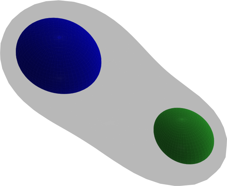
While hyperbolic relaxation methods are generally easier to implement and often more robust than direct elliptic solvers—particularly when given poor initial guesses—they are typically slower. As discussed in Sec. 4.1, locating the common horizon shown in Fig. 1 from a naïve initial guess takes over 10x longer with BHaHAHA than with AHFinderDirect. To close this performance gap, we implement OpenMP parallelization within BHaHAHA and introduce two new techniques within the hyperbolic relaxation framework. First, inspired by multigrid methods, we develop a strategy in which low-cost solutions on coarse grids serve as initial guesses for finer grids, accelerating convergence by more than 12x on 16 cores. Second, we incorporate an over-relaxation technique, adapted from numerical linear algebra, to further accelerate convergence. Together, these innovations reduce the runtime for BHaHAHA—when locating the challenging common horizon from scratch—to within about 10% of AHFinderDirect on 16 cores.
In the more common context of dynamically tracking horizons, BHaHAHA constructs a high-quality initial guess by extrapolating from up to three previous solutions. This accurate guess offers two key advantages. First, being close to the true solution, it significantly reduces the number of relaxation iterations. Second, it confines the search to a thick spherical shell around the expected horizon location rather than the full spherical volume. Since metric data must be interpolated from the source NR grids onto BHaHAHA’s spherical grid, reducing the search volume directly lowers the number of expensive interpolations—a major contributor to AH finder runtime. Together, these improvements significantly reduce overhead, enabling BHaHAHA to outperform AHFinderDirect by approximately 2.1x in dynamic AH tracking at comparable accuracy (Sec. 4.2).
The remainder of this paper is structured as follows. Section 2 reviews the mathematical foundations underlying BHaHAHA, while Sec. 3 details its algorithmic implementation. In Sec. 4, we present numerical results benchmarking BHaHAHA against AHFinderDirect in a range of scenarios, from horizon tracking to highly challenging single-horizon searches. Finally, Sec. 5 summarizes our findings and potential avenues for future enhancement of BHaHAHA.
2 Basic Equations
We adopt Einstein summation notation, with repeated Latin indices implying summation over the three spatial dimensions. The standard ADM (Arnowitt–Deser–Misner) 3+1 decomposition of the spacetime metric [46] is given by
| (1) |
where is the lapse function, the shift vector, and the spatial 3-metric. This decomposition naturally introduces spatial hypersurfaces characterized by an extrinsic curvature , defined by
| (2) |
where is the covariant derivative compatible with .
2.1 Expansion Function
An AH is defined as the outermost marginally outer trapped surface (MOTS) of a BH. Formally, a MOTS appears when the expansion function , which measures the rate of change of the area of an infinitesimal 2-surface along its outward normal, vanishes:
| (3) |
where is the outward unit normal to the MOTS, is the extrinsic curvature of the spatial hypersurface, and is its trace.
In practice, the MOTS is defined implicitly by a scalar level-set function given in spherical coordinates as
| (4) |
so that denotes the interior and the exterior of the MOTS. Since
| (5) |
the unit normal is obtained as
| (6) |
The full covariant divergence of is given by
| (7) |
where the partial divergence can be computed from Eq. 6 as
| (8) |
so that the full covariant divergence becomes
| (9) |
Combining these results, the expansion function is expressed as
| (10) |
which, given the definition of (Eq. 4), (Eq. 5), and (Eq. 6), along with the 3-metric , its derivatives, and the extrinsic curvature , constitutes a nonlinear elliptic PDE for .
2.2 Hyperbolic Relaxation Equations
Having cast the expansion function as a nonlinear elliptic PDE for (Eq. 10), we solve it using a hyperbolic relaxation scheme [35, 36]. The method evolves the system in a pseudo-time via the following damped wave equations:
| (11) |
where is a damping coefficient (units ) and is the relaxation wave speed (dimensionless, set to 1 in BHaHAHA). In the limit , the damping drives the system toward a steady state with , recovering .
2.3 Proper Area-Based MOTS Diagnostics
Integration over the MOTS is central to AH diagnostics. The infinitesimal area element is determined by the induced metric (where Greek indices run over angular coordinates ), computed from an embedding function that describes the surface in 3D Cartesian coordinates . For a MOTS given by in spherical coordinates centered at a Cartesian origin , the Cartesian coordinates of points on this surface are obtained via the standard spherical-to-Cartesian transformation (see Eqs. 16–18, with as the origin for the radial definition). The area element is then:
where is the determinant of the induced metric.
The induced metric is derived by pulling back the ambient 3D metric onto the 2D MOTS using the tangent vectors to the surface, , where :
| (12) |
Explicitly substituting and the derivatives of yields an expression for (cf. Eq. (24) in [27]):
| (13) | |||||
Here, the components are evaluated in spherical coordinates at (Eq. 4).
From this expression, the total MOTS area and irreducible mass are computed as:111Strictly speaking, the second equality holds in stationary spacetimes, but we follow convention in BHaHAHA and define the irreducible mass accordingly.
| (14) |
To update the MOTS location in BHaHAHA, we compute the centroid as the area-weighted average of the Cartesian position vector :
| (15) |
Using spherical coordinates centered at , the components of are given by the standard transformation:
| (16) | |||||
| (17) | |||||
| (18) |
We also compute the minimum, maximum, and mean radii relative to the centroid. The mean radius is defined as the area-weighted average of the Euclidean distance from the centroid:
| (19) |
where is the Kronecker delta.
2.4 Proper Circumference-Based MOTS Diagnostics
The spin of an isolated, nearly stationary BH can be estimated by computing proper circumferences along coordinate planes on the MOTS [20]. We define these via path integrals:
where denotes integration along a closed meridional path of constant , running from pole to pole and back along the MOTS. For numerical evaluation, the line element is interpolated along the path and integrated using high-order quadrature.
For spin aligned with the -axis, the dimensionless spin magnitude is determined from the polar-to-equatorial circumference ratio , with and . Following Alcubierre et al. [19], we invert
| (20) |
where is the complete elliptic integral of the second kind:
The inversion is performed via the Newton-Raphson algorithm, requiring both and its derivative, which depends on the complete elliptic integral of the first kind, .
3 Algorithmic Approach
Like its sister code NRPyElliptic [36], BHaHAHA is a simplified variant of the BlackHoles@Home [47] NR evolution code, generated by the open-source NRPy [43, 44] framework.222The version of BHaHAHA used in this paper can be generated from a Python environment, for example via the Linux command line, using pip install git+https://github.com/nrpy/nrpy.git@92a51d8 && python3 -m nrpy.examples.bhahaha, and following the emitted instructions. NRPy leverages SymPy [48] for symbolic computation and significantly extends its code generation capabilities, converting complex tensorial expressions (e.g., the expansion , Eq. 10) into highly optimized C code. BHaHAHA is implemented as a standalone AH finder library—the first of its kind—intended for general use in any NR code.333Instructions for implementing BHaHAHA into NR codes are provided in the NRPy repository, where BHaHAHA is housed.
The following sections outline the core steps of the BHaHAHA algorithm, detailing how it acquires and processes spacetime metric information from the host NR code, locates an AH using hyperbolic relaxation, and computes diagnostics on it.
3.1 Reading and Processing Metric Data
BHaHAHA requires the host NR code to provide the spatial metric, , and the extrinsic curvature, , in a Cartesian basis, interpolated onto BHaHAHA’s 3D cell-centered spherical grid. The grid’s origin must lie within the AH and fully enclose it. The grid may be configured either as a full sphere—for initial horizon finding—or as a spherical shell of nonzero thickness for subsequent tracking.
Although BHaHAHA seeks a 2D surface defined by , evaluating the expansion requires metric variables and their spatial derivatives at every point on the evolving trial surface in 3D. Performing full 3D interpolations from the host NR code onto at each relaxation step would be computationally prohibitive. To avoid this, BHaHAHA precomputes all necessary geometric quantities on a 3D spherical grid that shares the same angular resolution as . This arrangement enables rapid 1D interpolation along radial spokes (i.e., in at fixed ) to obtain metric data on the trial surface throughout the relaxation process.
After the host NR code interpolates the 12 independent ADM quantities ( and ) onto BHaHAHA’s grid, BHaHAHA transforms them into conformal BSSN variables expressed in the spherical basis. BSSN variables are used instead of ADM largely for convenience, as they are already implemented within the reference-metric formalism in NRPy. To ensure numerical stability, the singular parts of tensor components in this formalism are handled analytically, so that only the regular (nonsingular) parts are ever interpolated or finite-differenced [41, 42, 44].
To compute , all required BSSN variables and first spatial derivatives must be available for interpolation onto the surface at each pseudo-time step. These derivatives (both angular and radial) are computed on the 3D grid using sixth-order finite differencing, employing appropriate boundary conditions (for angular derivatives: parity conditions at poles and ; for radial derivatives upwind/downwind stencils at radial boundaries). These precomputed fields are stored on the 3D spherical grid, ready for 1D radial interpolations onto the trial AH surface.
3.2 Hyperbolic Relaxation Formulation
As introduced in Sec. 2.2, BHaHAHA finds a marginally outer trapped surface (MOTS) by evolving the hyperbolic relaxation system defined in Eq. 11. In these equations, the function represents the trial surface radius on BHaHAHA’s spherical grid, while the auxiliary field serves as a radial velocity-like component during the pseudo-time evolution. For simplicity, the relaxation wave speed is set to unity () in this implementation.444In NRPyElliptic [36], setting to the maximum value allowed by the CFL condition significantly accelerated convergence on prolate spheroidal grids. However, because BHaHAHA uses a spherical angular grid, which exhibits only mild variations in grid spacing from poles to equator, we found this optimization to be ineffective here.
The damping term in the equation for drives the system toward the steady-state condition . As the system relaxes and also approaches zero, the second equation enforces the desired MOTS condition .
To ensure dimensional consistency and achieve scale-invariant behavior independent of the BH’s coordinate mass, the user provides a characteristic BH mass scale and specifies the dimensionless damping coefficient . Internally, BHaHAHA computes so that the damping term carries the correct physical units.
3.3 Initial Data
When no prior guess is provided, BHaHAHA employs a default spherical guess , where is the user-specified maximum radius of the spherical search volume. For subsequent finds (tracking), BHaHAHA constructs an initial guess at by extrapolating data from up to three previous horizon configurations. Lagrange extrapolation of up to second order (depending on the number of available prior configurations) is consistently applied to all quantities. This algorithm predicts: (i) the new centroid from prior centroid locations ; (ii) the expected radial extent from prior radial bounds; and (iii) the horizon shape function pointwise from the prior shapes . The predicted radial extent defines a thick spherical shell onto which the host code interpolates metric data, significantly reducing expensive interpolations compared to using a full spherical volume. The extrapolated shape serves as the initial guess, denoted , for the pseudo-time evolution described by Eq. 11.
3.4 Pseudo-Time Evolution
The system Eq. 11 is integrated forward in pseudo-time using the standard third-order Strong Stability Preserving Runge-Kutta (SSPRK3) scheme [49]. The pseudo-time step is determined by a Courant-Friedrichs-Lewy (CFL) condition based on the wave speed and the proper grid spacings on the evolving surface, and . SSPRK3 was selected after empirical testing showed it permitted a slightly higher CFL factor (1.0) than other methods considered, without increasing computational cost.
Evaluating the right-hand side of Eq. 11, specifically the term, requires the precomputed metric quantities and their derivatives (Sec. 3.1) on the current trial surface . Since this surface generally does not align with the radial grid points of BHaHAHA’s internal 3D grid, these quantities are obtained via interpolation. A key optimization is performed: at the start of each full pseudo-time step (before the first SSPRK3 substep), BHaHAHA performs high-order 1D Lagrange interpolation along radial spokes for each angular grid point , mapping the required precomputed fields from the 3D grid onto the trial surface .
These interpolated values are cached and reused during all subsequent SSPRK3 substeps within that pseudo-time step. This strategy dramatically reduces computational cost compared to repeated 3D interpolations, while maintaining high-order accuracy. Only the angular derivatives of the evolving shape function (needed for ) are recomputed at each SSPRK3 substep using high-order finite differencing, as itself changes within the Runge-Kutta integration.
3.5 Stop Conditions
This pseudo-time evolution proceeds until the trial surface sufficiently satisfies the condition . To determine convergence, BHaHAHA employs physically meaningful and scale-invariant criteria.
Because has dimensions of inverse mass (or inverse length in units), requiring the norm of to be less than would be far more stringent for a BH with coordinate mass than for one with mass . To ensure consistent convergence behavior across a broad range of systems—including high mass ratio binaries—BHaHAHA requires the user to specify a characteristic mass scale for each BH. All convergence criteria are then defined in terms of the dimensionless product .
To our knowledge, BHaHAHA is the first general-purpose AH finder to explicitly incorporate ’s dimensionality into its stopping conditions, a critical step for ensuring robustness regardless of arbitrary overall mass scale or mass ratio.
Convergence is declared and relaxation terminated when both of the following criteria are satisfied:
| (21) |
where and denote the and norm over the angular grid, respectively. The default tolerances are and . This is consistent with the general preference to adopt norms as thresholds for convergence. This said, the tolerances can be adjusted to prioritize averaged accuracy if desired. In typical scenarios, we have never observed and norms to differ by more than a factor of a few. By comparison AHFinderDirect adopts , but as shown in Sec. 4.2, the extra orders of magnitude offer no benefit for typical horizon finds.
3.6 Convergence Acceleration Techniques
Although hyperbolic relaxation is robust, its convergence is limited by the CFL condition, with computational cost scaling as roughly for a -dimensional surface ( here) discretized with points per dimension. To mitigate this, BHaHAHA typically operates at modest angular resolution (defaulting to ), made effective by its use of high-order numerical methods (sixth-order finite differencing, Sec. 3.1, and fifth-order Lagrange interpolation). As shown in Sec. 4, BHaHAHA achieves comparable accuracy to the fourth-order AHFinderDirect [11] at their respective default resolutions and tolerances. To further accelerate convergence towards the state defined by the termination criteria (Sec. 3.5), BHaHAHA introduces two techniques new to hyperbolic relaxation solvers:
3.6.1 Multigrid-Inspired Relaxation
BHaHAHA implements a relaxation strategy inspired by multigrid methods, but tailored to hyperbolic evolution. Rather than transferring residuals between resolution levels as in standard multigrid elliptic solvers, BHaHAHA focuses on generating progressively better initial guesses. It first relaxes the system on a coarse angular grid (e.g., points), where convergence is rapid due to the small number of grid points and the relatively large pseudo-time step permitted by the CFL condition. The resulting solution is then prolonged to the next finer grid (e.g., ) via fifth-order interpolation and used as an initial guess. This hierarchy may continue up to the target resolution (e.g., ), with each finer level requiring significantly fewer iterations due to the improved starting point. The 3D spherical source grid containing BSSN data (Sec. 3.1) is prepared once per resolution level. These data are initially interpolated from the host code at the highest angular resolution; for coarser levels, the required 3D BSSN fields (including derivatives) are downsampled (interpolated) versions of high-resolution data.
3.6.2 Over-Relaxation
During pseudo-time evolution, the early wavelike behavior of the hyperbolic system generally gives way to a slower, asymptotic approach toward the solution. To accelerate convergence in this phase of the evolution, BHaHAHA periodically attempts over-relaxation. It stores a prior shape (at pseudo-time ) and extrapolates from the current shape (at ) via
for extrapolation factors chosen in geometric progression. For each trial shape, BHaHAHA interpolates the metric quantities via 1D radial spokes and computes the expansion . The shape minimizing is selected. If it provides a significant improvement over , the system is updated: is replaced by , is reset to , metric data are interpolated to the new trial surface, and the CFL-limited timestep is recalculated.
3.7 Diagnostics Computation
Upon successful convergence (i.e., when criteria Eq. 21 are satisfied), BHaHAHA computes several diagnostic quantities to provide key physical parameters characterizing the BH at that moment in time, as well as verify the accuracy of the horizon found by BHaHAHA (i.e., norms of ):
-
•
Area & Mass: The proper surface area is computed by integrating the area element over the surface , where is the determinant of the induced 2-metric on the horizon (Eq. 13). The irreducible mass is then estimated as (exact for stationary horizons).
-
•
Centroid & Radii: The coordinate centroid of the horizon surface is computed using Eq. 15. The minimum, maximum, and mean coordinate radii relative to this centroid are also reported.
-
•
Spin (via Circumferences): The proper equatorial circumferences in the coordinate planes passing through the centroid () are computed. These are used to estimate the magnitude of the dimensionless spin components by numerically inverting the Kerr spin-circumference relations given in Eq. 20.
-
•
Expansion Norms: The final and norms of the dimensionless expansion are used to determine whether termination criteria were met.
4 Results
We compare BHaHAHA’s performance, robustness, and accuracy with the widely used AHFinderDirect across several challenging scenarios that showcase its key innovations and utility as a general-purpose AH finder. Section 4.1.1 evaluates the performance gains from BHaHAHA’s acceleration strategies and OpenMP parallelization using a demanding common horizon search with a poor initial guess. Section 4.1.2 tests the scale invariance of BHaHAHA and AHFinderDirect by repeating this search across BH total masses spanning 16 orders of magnitude. While such single-slice tests serve as useful benchmarks, AH finders are more commonly used for tracking horizons in dynamical spacetimes. To this end, Sec. 4.2 assesses BHaHAHA’s performance during a BBH inspiral and merger, identifying the tolerances required to match typical AHFinderDirect errors. Finally, Sec. 4.3 shows that at high resolutions BHaHAHA matches AHFinderDirect and other finders to many significant digits in a precision 3-BH common horizon search, further demonstrating its infrastructure independence through implementation in the BlackHoles@Home NR code.
4.1 BHaHAHA vs. AHFinderDirect Performance Comparison: BBH Merger
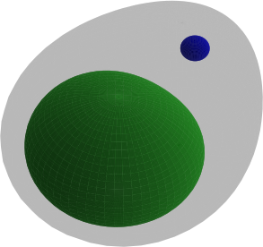
To assess the acceleration techniques of Sec. 3.6, the ET implementation of BHaHAHA is used to locate both individual and common MOTSs on a two-BH zero-momentum Brill–Lindquist [50] spacetime slice with bare masses and , placed at and , respectively. This setup yields the individual and common MOTSs plotted in Fig. 1.
The configuration is made intentionally challenging for AH finders. The large mass ratio creates a highly non-spherical common horizon, and the axis of symmetry is tilted from BHaHAHA’s -axis. Both BHaHAHA and AHFinderDirect are given the same poor initial guesses: three spherical trial surfaces centered on the massive puncture (radius 0.4), the less massive one (radius 0.1), and the common horizon (radius 0.9), with the latter centered at the origin —far from its true location.
4.1.1 Impact of Multigrid and Over-Relaxation Accelerations on BHaHAHA Performance Compared to AHFinderDirect
We establish a baseline by comparing the performance of unmodified BHaHAHA to that of AHFinderDirect in locating the common horizon, using the same poor, origin-centered spherical initial guess. At the default resolution (), unaccelerated BHaHAHA is significantly slower than the serial AHFinderDirect,555AHFinderDirect, as implemented in the ET via AHFinderDirect, is not parallelized with OpenMP. requiring 10–52x more wall-clock time depending on CPU core count (Table 1, first row). Its convergence from the poor initial guess (Fig. 2, solid blue line) begins with wave-like transients and variable damping, followed by steady exponential decay. Fitting this late-time decay (dotted black line) gives an e-folding period of total gridpoint evaluations of (GEs). Reaching the target tolerance (horizontal dotted line) requires approximately GEs.
-
Number of Cores 1 2 4 8 16 BHaHAHA no accel total 73.0 37.6 21.1 14.6 20.6 BHaHAHA OR total 19.9 10.7 6.06 4.43 5.81 BHaHAHA MG total 4.01 2.47 1.71 1.38 1.70 BHaHAHA MG & OR 3D interp 0.54 0.60 0.66 0.67 0.69 horizon find 2.28 1.22 0.68 0.47 0.65 total 2.82 1.82 1.34 1.14 1.34 AHFinderDirect total 1.41 1.41 1.44 1.44 1.48
The multigrid-inspired strategy (Sec. 3.6.1) substantially boosts performance. It solves the problem on successively finer grids—, , and —with each solution initializing the next. This hierarchy accelerates convergence, as achieving convergence on coarse grids is inexpensive: just and of the GEs per iteration compared to . As shown in Fig. 2 (green dash-dot line), the method achieves a tolerance using only of the GEs required by unaccelerated BHaHAHA. Wall-clock time improves by 11–18x across 1–16 cores (Table 1), cutting single-core runtime from 73.0 s to 4.01 s. Jagged features in the convergence plot mark grid resolution transitions.
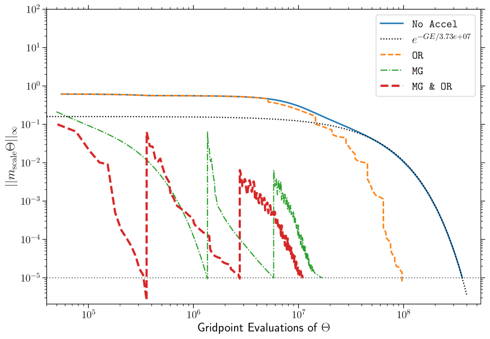
The over-relaxation technique alone (Sec. 3.6.2) provides a modest 3.3–3.7x speedup across 1–16 cores (Fig. 2, orange dashed line; Table 1), reducing single-core runtime from 73.0 s to 19.9 s. This approach is generally less effective at improving performance than the multigrid-inspired strategy.
Combining periodic over-relaxation with multigrid yields the highest performance boost (Fig. 2, thick dashed red line), achieving a tolerance in GEs. This strategy offers a 13–26x speedup across 1–16 cores, lowering the single-core runtime to 2.82 s (Table 1).
Comparing parallel scaling of fully accelerated BHaHAHA (‘BHaHAHA MG & OR’) to serial AHFinderDirect yields additional insight. On one core, BHaHAHA takes 2.82 s—twice the time of AHFinderDirect (1.41 s)—but with the aid of OpenMP scaling is able to reduce runtime to 1.14 s on 8 cores. This outperforms AHFinderDirect’s 1.44 s by . At 16 cores, BHaHAHA slows to 1.34 s, slightly above its 8-core time, likely due to increased OpenMP overhead due to overdecomposition on the grid.
A breakdown of BHaHAHA’s timing (‘BHaHAHA MG & OR’, Table 1) better illustrates its scaling with increased core count. While the ‘horizon find’ computation scales well to 8 cores, the ‘3D interp’ phase—interpolating from the ET Carpet AMR grid [51, 52] to BHaHAHA’s spherical grid—dominates runtime and scales poorly, limiting overall speedup.
4.1.2 Scale Invariance: BHaHAHA vs. AHFinderDirect
Since Einstein’s equations in vacuum are scale-invariant, robustness to total mass scale is a key test of AH finders: rescaling mass () and coordinates () maps solutions to other valid ones. Thus dimensionless quantities like should remain constant. We test this using nonspinning Brill–Lindquist BBH data (Sec. 4.1), rescaling the puncture masses so that spans to . Grid spacing is scaled proportionally () to keep fixed.
At each scale, both BHaHAHA and AHFinderDirect find the common horizon and inner MOTSs. We compute the normalized areas , (larger mass), and (smaller mass). BHaHAHA uses a scale-invariant convergence criterion , while AHFinderDirect uses an absolute tolerance chosen for consistency.
As shown in Table 2, the finders agree well across : and match to five digits; to four. Outside this range, BHaHAHA maintains six-digit accuracy across all 16 orders of magnitude, confirming scale invariance. AHFinderDirect, however, fails for (missing horizons) and diverges for , with deviating by up to 18% at . This suggests AHFinderDirect’s absolute tolerance may cause false convergence at large due to premature settling near the initial guess.
| Mass Scale () | Common () | Inner 1 () | Inner 2 () | |||
|---|---|---|---|---|---|---|
| BAH | AHFD | BAH | AHFD | BAH | AHFD | |
| 50.1715 | NF | 46.5112 | NF | 6.58904 | NF | |
| 50.1715 | 50.1713 | 46.5112 | 46.5111 | 6.58904 | NF | |
| 50.1715 | 50.1713 | 46.5112 | 46.5111 | 6.58904 | 6.58938 | |
| 1 | 50.1715 | 50.1713 | 46.5112 | 46.5111 | 6.58904 | 6.58938 |
| 50.1715 | 50.1713 | 46.5112 | 46.5111 | 6.58904 | 6.58938 | |
| 50.1715 | 58.9557 | 46.5112 | 46.5192 | 6.58904 | 7.47378 | |
| 50.1715 | 58.9557 | 46.5112 | 47.0723 | 6.58904 | 7.30382 | |
4.2 Dynamical Horizon Study: GW150914
Having established BHaHAHA’s robustness to challenging horizon finds on a single spacetime slice, we next evaluate its performance in a fully dynamical setting: an NR simulation of the GW150914-like BBH merger from the ET gallery [53, 54].
The simulation makes use of the best-fit priors from GW150914 [1, 55] with a mass ratio , aligned spins and , and initial separation , with total mass . The initial data is computed using ET’s TwoPunctures thorn [56, 57], with a resolution of () to minimize initial constraint violations. The gauge is initialized with and .
The evolution uses the BSSN formalism implemented in BaikalVacuum [44, 57] with the moving-puncture gauge (1+log lapse, Gamma-driver shift). Numerical methods include 8th-order spatial differencing, RK4 time integration, and 9th-order Kreiss–Oliger dissipation (strength 0.15). Punctures are tracked using the PunctureTracker thorn and AMR is managed by Carpet [51, 52] using 11 refinement levels (factor 2) and an outer boundary of . The finest resolution is . Subcycled time integration uses a CFL factor of 0.45, with timestep ratios: . Full parameters may be found in the ET_BHaHAHA thorn.666The ET_BHaHAHA thorn used in this paper is available in the EinsteinAnalysis repository at https://bitbucket.org/einsteintoolkit/einsteinanalysis, commit ID b306cb. The parameter file used for this example can be found at ET_BHaHAHA/par/GW150914_baikalvacuum.par.
To make the testbed more challenging, we adopt standard moving puncture methods, deliberately omitting recent noise-suppression techniques [47] that can reduce constraint violations on AMR grids in BBH simulations by orders of magnitude. Both BHaHAHA and the standard AHFinderDirect [11, 58] concurrently track AHs, searching every 44 base iterations (). Initially, each identifies two separate horizons.
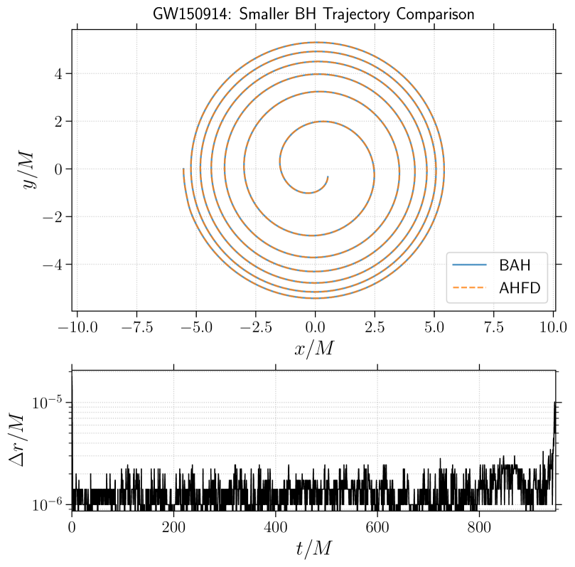
Figure 3 illustrates the inspiral dynamics. The top panel shows the smaller black hole’s AH centroid trajectory as computed independently by BHaHAHA and AHFinderDirect during the orbits preceding common horizon formation. The trajectories are visually indistinguishable, indicating strong agreement. The bottom panel quantifies this, showing their Euclidean separation remains near , confirming the high precision of both finders.
For dynamic tracking, BHaHAHA employs three multigrid levels (, , ), over-relaxation, quadratic extrapolation from up to three prior solutions to estimate the initial shape and centroid, and optimized spherical shell search domains to reduce interpolation costs from the host NR code.
While these features substantially improve BHaHAHA’s performance, they must be evaluated against accuracy constraints: tolerances required to ensure agreement with AHFinderDirect. As we will show, interpolating metric quantities ( and ) from the ET AMR grid introduces a systematic error. Both finders rely on this interpolation to compute derivatives used in evaluating the expansion , leading to an error floor of approximately .
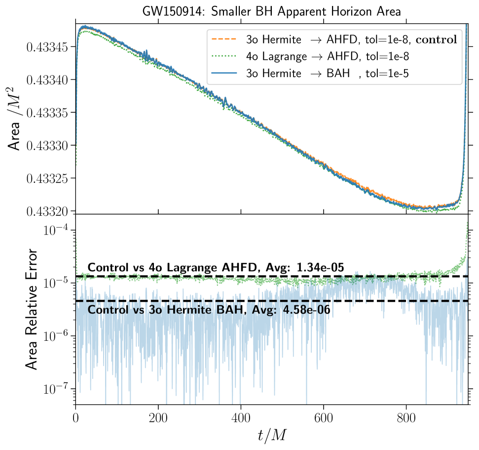
To measure the impact of interpolation error from the host NR code, in Fig. 4, we plot the area of the smaller horizon throughout the entire inspiral using three different approaches. First, AHFinderDirect at default tolerance using the ET’s 3rd-order Hermite interpolation algorithm (control). Second, an identically configured AHFinderDirect, except instead of Hermite, the ET’s 4th-order Lagrange interpolation algorithm is used. Third, BHaHAHA is run with its default tolerance of .
As shown in the bottom panel of Fig. 4, comparing AHFinderDirect with Hermite versus Lagrange interpolation reveals an average relative area difference of . This difference, consistent with the general accuracy of AHFinderDirect reported in the abstract of the AHFinderDirect announcement paper [11], establishes an acceptable relative error floor for our comparisons.
At its default tolerance and using the ET’s 3rd-order Hermite interpolation, BHaHAHA demonstrates excellent agreement with the control run (top panel, Fig. 4). Its average relative area error of is comfortably below the interpolation error floor.
Applying the same error analysis approach illustrated in Fig. 4, we conduct a detailed error analysis on both and norms of in Tables 3 and 4.
| Description | Runtime (s) | |
|---|---|---|
| Input Metric Interp. Error (AHFD) | 500. | |
| BAH | 201 | |
| BAH | 204 | |
| BAH | 256 | |
| BAH | 293 |
| AHFD Error | BAH Error | AHFD; BAH | |
|---|---|---|---|
| Description | () | () | Runtime (s) |
| Input Metric Interp. Error (AHFD) | N/A | 500.; — | |
| AHFD & BAH | 359; 193 | ||
| AHFD & BAH | 494; 240 | ||
| AHFD & BAH | 494; 333 | ||
| AHFD & BAH | 497; 559 | ||
| AHFD & BAH | 501; 870 |
Tightening BHaHAHA’s tolerance (), while keeping loose, reduces the relative area error until it saturates at for (Table 3). For AHFinderDirect, reducing the tolerance improves precision to at (Table 4), but this is artificial, as it relies on identical metric data (provided via 3rd-order Hermite interpolation) from the host NR grid. Similarly, BHaHAHA’s error plateaus at when only the constraint is tightened.
Comparing the convergence of and norms (Tables 3, 4), both saturate around , limited by interpolation from the NR host grid. However, reaches this limit more efficiently. For instance, BHaHAHA achieves in 256s with , while needs and 333s to reach .
At practical tolerances (), still slightly outperforms: BHaHAHA yields in 204s versus in 240s for , both well below the interpolation error floor. Thus, interpolation-limited accuracy is achieved with either norm at —unlike AHFinderDirect, which often uses unnecessarily strict tolerances ().
While enforces strict local accuracy, better optimizes average accuracy and is less sensitive to outliers. However, in keeping with the stop conditions used by most other AH finders, we generally adopt in this work. In practice, the norms agree to within a factor of a few. Thus, by setting BHaHAHA’s defaults to and , we effectively disable the condition in favor of .
At tolerances, BHaHAHA significantly outperforms AHFinderDirect. In GW150914-like inspirals run on a single AMD EPYC 9654 (96-core) node using 8 MPI ranks and 12 OpenMP threads per rank, BHaHAHA achieves interpolation-limited accuracy () in 204–240 seconds, compared to 494 seconds for AHFinderDirect at similar error levels. At stricter tolerances (–), beyond the interpolation limit, AHFinderDirect becomes more efficient as BHaHAHA saturates. The scaling studies presented in Sec. 4.1.1 and Table 1 show that BHaHAHA performs optimally at around 8–16 OpenMP threads. Thus, the 12-thread configuration used here is nearly ideal. Even with fewer threads, however, BHaHAHA would likely retain a substantial speed advantage over AHFinderDirect at standard simulation tolerances.
BHaHAHA’s efficiency at practical tolerances has important implications for large-scale simulations. Since each MPI rank performs one horizon search, the per-node speedup translates directly into reduced overall cost. For standard BBH evolutions at tolerance, BHaHAHA reduces horizon-finding wall time by roughly a factor of two compared to AHFinderDirect, without compromising accuracy. This speedup is easily achieved by enabling the BHaHAHA thorn and choosing appropriate tolerances, with no other changes to the existing ET workflow.
4.2.1 Automatic Triggering of Common Horizon Searches: BHaHAHA’s BBH Mode
AHFinderDirect requires specifying in advance when and where to search for a common horizon—a nontrivial task, especially for BBH mergers occurring away from the origin. To address this, BHaHAHA’s ET implementation includes an experimental “BBH mode” that automatically schedules common horizon searches based on the centroids and radii of individual AHs.
In this GW150914-inspired simulation, “BBH mode” scheduled a common-horizon search at iteration 75680 (), and BHaHAHA subsequently detected the common horizon shown in Fig. 5 at iteration 75944 (). For direct comparison, AHFinderDirect, manually triggered to begin common-horizon searches at iteration 75680 as well, also first detected the common horizon at exactly iteration 75944.
To improve robustness during the highly dynamical early phase of a just-formed common horizon, “BBH mode” doubles the multigrid resolution at the lowest refinement level, raises the iteration ceiling, reduces the CFL factor by 10%, and uses a large fixed-radius initial guess for the first three horizon searches.
Although currently experimental, the implementation of “BBH mode” within the ET serves as a template for integrating it into other NR codes. Future work includes porting it to the BlackHoles@Home NR code and enhancing its robustness across a wider range of BBH scenarios.
4.3 Precision Horizon Finding: Three-BH Critical Radius
Thus far, we have demonstrated that results from BHaHAHA and AHFinderDirect generally agree to within 5–7 significant digits (Secs. 4.1.2 and 4.2), a level primarily limited by metric-interpolation errors from the ET’s Cartesian grids. To investigate whether BHaHAHA can achieve even higher accuracy and match other AH finders’s results at greater precision, we focus here on a more demanding benchmark.
This test also serves to demonstrate BHaHAHA’s infrastructure independence. Here, we use its implementation within the BlackHoles@Home NR code [44, 47, 43], rather than the ET [34, 54] framework used previously. Notably, BlackHoles@Home employs 8th-order finite differencing and 7th-order interpolation, compared to 6th- and 5th-order schemes in ET. This higher-order approach and optimized grid support improved precision.
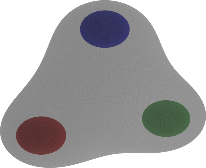
The benchmark problem is the three-black-hole “critical-radius” configuration described by Thornburg [11]. As shown in Fig. 6, three equal-mass Brill–Lindquist punctures (each with bare mass , total mass ) are placed in an equilateral triangle centered at the origin. The task is to find the largest separation admitting a common AH. This critical value, , is a longstanding test for AH finders [11, 27].
To isolate BHaHAHA’s intrinsic accuracy and reduce metric-interpolation error, spacetime data are sampled from a high-resolution SinhSpherical grid native to BlackHoles@Home. This grid uses a uniform angular resolution of and 320 exponentially spaced radial points,777Radial points follow [44], with , . efficiently resolving the smooth tri-nodal horizon. Internally, BHaHAHA was tested at increasing multigrid resolutions (, , ) with a strict convergence criterion: , where for this system.
Using a bisection-style search,888The search sampled radii uniformly between and (code units). At each step, trial radii were evaluated in parallel on six nodes (two per node). was bracketed to:
This lies well within the Richardson-extrapolated value from Thornburg using AHFinderDirect [11], and matches the recent reported by Hui & Lin [27], who used a Cartesian-grid-based multigrid solver in the ET with tolerance . Our effective tolerance of (i.e., ) is about 2.3 times stricter.
Although depends on the convergence tolerance—tighter criteria yield smaller values due to the monotonic decrease of near the MOTS—the agreement across AH finders is excellent. These results demonstrate that, when supplied with high-resolution data and operated at strict tolerances, BHaHAHA achieves agreement with established AH finders to at least 8 significant digits, even in this demanding test case.
5 Conclusions and Future Work
We have introduced BHaHAHA, the BlackHoles@Home Apparent Horizon Algorithm, the first open-source, infrastructure-agnostic library for AH finding in NR. BHaHAHA reformulates the elliptic MOTS equation as a damped nonlinear scalar wave equation on a 2-sphere, using a reference-metric formulation to manage coordinate singularities. It is the first method to use hyperbolic-relaxation flow for AH finding, and inherits the robustness of flow methods to poor initial guesses.
While hyperbolic relaxation is robust, it is typically slower than elliptic solvers. BHaHAHA mitigates this with two key strategies: a multigrid-like refinement that seeds fine-grid solves from coarse-grid solutions, and an over-relaxation technique adapted from numerical linear algebra. In addition, BHaHAHA is OpenMP parallelized to scale across modern multicore CPUs.
These enhancements were critical for performance. In a challenging common horizon test case (Sec. 4.1.1, Fig. 1), they reduced total grid-point evaluations by over 90% and achieved up to 26x speedups on eight cores over a naïve single-core implementation. Further, BHaHAHA outperformed the serial AHFinderDirect by 21% on 8 cores and 9.5% on 16 cores, though it remained about twice as slow on a single core (Table 1).
When tracking horizons in dynamical spacetimes, the accuracy of AH finders is typically limited by interpolation errors when transferring metric data from the host NR grid. For the GW150914-like BBH inspiral of Sec. 4.2, these errors lead to relative horizon area discrepancies of as observed with AHFinderDirect (Fig. 4), consistent with the accuracy reported in the abstract of the AHFinderDirect announcement paper [11]. With similar tolerances, BHaHAHA—using extrapolated initial guesses and optimized interpolation—runs 2.1x faster than AHFinderDirect. At its default tolerance , BHaHAHA yields relative area errors of and horizon trajectories agreeing with AHFinderDirect to within (Fig. 3), showing that BHaHAHA’s speed advantage does not compromise accuracy.
A key strength of BHaHAHA is its invariance to overall system scale: all dimensionful tolerances and parameters are set relative to each horizon mass. This allows BHaHAHA to reliably compute normalized horizon areas across 16 orders of magnitude in mass—a regime where the tested AHFinderDirect implementation fails or deviates significantly (Sec. 4.1.2, Table 2).
Precision tests of the three-throat Brill–Lindquist configuration (Sec. 4.3) show that BHaHAHA, when run with high internal resolution and strict tolerances, reproduces the value of obtained by other state-of-the-art AH finders to all significant digits.
Being an infrastructure-agnostic library, BHaHAHA has been successfully integrated into both the ET and BlackHoles@Home NR frameworks, demonstrating its adaptability. These results further establish hyperbolic relaxation as a fast, accurate, and scale-invariant method for AH finding—combining the robustness of flow-based approaches with performance that matches or exceeds that of AHFinderDirect.
Looking ahead, several developments will enhance BHaHAHA’s capabilities. Planned improvements to the BlackHoles@Home and ET implementations include spatial masking, allowing horizon interiors to be excised or GRHD/GRMHD fields quenched inside black holes. We aim to make the BBH mode more robust for automatic common horizon detection in both the ET and BlackHoles@Home. Efforts are also underway to integrate BHaHAHA into additional NR infrastructures beyond the ET and BlackHoles@Home.
Performance and algorithmic optimizations are also a priority. A major goal is to enable GPU support for BHaHAHA, building on recent success running NRPyElliptic on CUDA-enabled GPUs [37]. We also plan to explore new grid structures, such as tilted ellipsoidal coordinates, to better sample spacetime fields around spinning black holes. On the physics front, we plan to implement the isolated- and dynamical-horizon formalisms [59, 60, 22] to enable advanced quasi-local diagnostics (e.g., spin, mass, and energy or angular momentum fluxes).
The foundational role of hyperbolic relaxation in NR, established decades ago with the Gamma-driver shift conditions [38, 39], has paved the way for its application in standalone initial-data solvers [35, 36, 37]. BHaHAHA’s success in AH finding further demonstrates the power of this approach for solving elliptic PDEs in NR. Crucially, its multigrid-inspired and over-relaxation techniques are broadly applicable and poised to enhance performance across other current and potential hyperbolic relaxation applications, such as initial-data construction, constraint damping, and inverse-curl operations [61]. We aim to continue developing BHaHAHA and explore the application of its acceleration techniques to other key problems in NR.
Acknowledgments
We would like to thank W. K. Black, S. Brandt, P. Diener, M. Fernando, R. Haas, N. Jadoo, B. J. Kelly, S. T. McWilliams, J. Miller, S. C. Noble, E. Schnetter, H. Sundar, and several others for helpful discussions in the preparation of this manuscript. Z.B.E. gratefully acknowledges support from NSF awards PHY-2110352/2508377, PHY-2409654, OAC-2004311/2227105, OAC-2411068, and AST-2108072/2227080, as well as NASA awards ISFM-80NSSC18K0538, TCAN-80NSSC18K1488, and ATP-80NSSC22K1898. TA is thankful for support from NSF grants OAC-2229652 and AST-2108269. L.R.W. gratefully acknowledges support from NASA award LPS-80NSSC24K0360. Z.B.E. and ST received additional support from NASA award ATP-80NSSC22K1898 and the University of Idaho P3-R1 Initiative. This research made use of the resources of the High Performance Computing Center at Idaho National Laboratory, which is supported by the Office of Nuclear Energy of the U.S. Department of Energy and the Nuclear Science User Facilities under Contract No. DE-AC07-05ID14517. In addition, it made use of the Falcon [62] supercomputer, operated by the Idaho C3+3 Collaboration.
References
References
- [1] Abbott B P et al. (LIGO Scientific, Virgo) 2016 Phys. Rev. Lett. 116 061102 (Preprint 1602.03837)
- [2] Abbott T D et al. (LIGO Scientific, Virgo) 2016 Phys. Rev. X 6 041014 (Preprint 1606.01210)
- [3] Abbott B P et al. (LIGO Scientific, Virgo) 2019 Phys. Rev. X 9 031040 (Preprint 1811.12907)
- [4] Abbott R et al. (LIGO Scientific, Virgo) 2021 Phys. Rev. X 11 021053 (Preprint 2010.14527)
- [5] Abbott R et al. (LIGO Scientific, VIRGO) 2024 Phys. Rev. D 109 022001 (Preprint 2108.01045)
- [6] Abbott R et al. (KAGRA, VIRGO, LIGO Scientific) 2023 Phys. Rev. X 13 041039 (Preprint 2111.03606)
- [7] LIGO Scientific Collaboration and Virgo Collaboration (Virgo, LIGO Scientific) 2017 Phys. Rev. Lett. 119 161101:1–18 (Preprint 1710.05832)
- [8] Abbott B P et al. (LIGO Scientific, Virgo, Fermi GBM, INTEGRAL, IceCube, AstroSat Cadmium Zinc Telluride Imager Team, IPN, Insight-Hxmt, ANTARES, Swift, AGILE Team, 1M2H Team, Dark Energy Camera GW-EM, DES, DLT40, GRAWITA, Fermi-LAT, ATCA, ASKAP, Las Cumbres Observatory Group, OzGrav, DWF (Deeper Wider Faster Program), AST3, CAASTRO, VINROUGE, MASTER, J-GEM, GROWTH, JAGWAR, CaltechNRAO, TTU-NRAO, NuSTAR, Pan-STARRS, MAXI Team, TZAC Consortium, KU, Nordic Optical Telescope, ePESSTO, GROND, Texas Tech University, SALT Group, TOROS, BOOTES, MWA, CALET, IKI-GW Follow-up, H.E.S.S., LOFAR, LWA, HAWC, Pierre Auger, ALMA, Euro VLBI Team, Pi of Sky, Chandra Team at McGill University, DFN, ATLAS Telescopes, High Time Resolution Universe Survey, RIMAS, RATIR, SKA South Africa/MeerKAT) 2017 Astrophys. J. Lett. 848 L12 (Preprint 1710.05833)
- [9] Penrose R 1965 Phys. Rev. Lett. 14 57–59
- [10] Senovilla J M M 2011 Int. J. Mod. Phys. D 20 2139 (Preprint 1107.1344)
- [11] Thornburg J 2004 Class. Quant. Grav. 21 743–766 (Preprint gr-qc/0306056)
- [12] Garfinkle D 2002 Phys. Rev. D 65 044029 (Preprint gr-qc/0110013)
- [13] Pretorius F 2005 Class. Quantum Grav. 22 425–451 (Preprint gr-qc/0407110)
- [14] Duez M D, Shapiro S L and Yo H J 2004 Phys. Rev. D 69 104016 (Preprint gr-qc/0401076)
- [15] Hawke I, Loffler F and Nerozzi A 2005 Phys. Rev. D 71 104006 (Preprint gr-qc/0501054)
- [16] Etienne Z B, Liu Y T, Paschalidis V and Shapiro S L 2012 Phys. Rev. D 85 064029 (Preprint 1112.0568)
- [17] Zilhão M and Löffler F 2013 Int. J. Mod. Phys. A 28 1340014 (Preprint 1305.5299)
- [18] Christodoulou D 1970 Phys. Rev. Lett. 25 1596–1597
- [19] Alcubierre M et al. 2005 Phys. Rev. D 72 044004 (Preprint gr-qc/0411149)
- [20] Smarr L 1973 Phys. Rev. D 7 289–295
- [21] Brandt S R and Seidel E 1995 Phys. Rev. D 52 870–886 (Preprint gr-qc/9412073)
- [22] Ashtekar A and Krishnan B 2004 Living Rev. Rel. 7 10 (Preprint gr-qc/0407042)
- [23] Thornburg J 2007 Living Rev. Rel. 10 3 (Preprint gr-qc/0512169)
- [24] França T 2023 Binary Black Holes in Modified Gravity Ph.D. thesis Queen Mary, U. of London (main) (Preprint 2308.12037)
- [25] Andrade T et al. 2021 J. Open Source Softw. 6 3703 (Preprint 2201.03458)
- [26] 2025 GRChombo GitHub repository https://github.com/GRTLCollaboration/GRChombo
- [27] Hui H K and Lin L M 2025 Class. Quant. Grav. 42 055008 (Preprint 2404.16511)
- [28] Gundlach C 1998 Phys. Rev. D 57 863–875 (Preprint gr-qc/9707050)
- [29] Fernando M, Neilsen D, Zlochower Y, Hirschmann E W and Sundar H 2023 Phys. Rev. D 107 064035 (Preprint 2211.11575)
- [30] 2025 Dendro-GR GitHub repository https://github.com/paralab/Dendro-GR
- [31] Kidder L E, Field S E, Foucart F, Schnetter E, Teukolsky S A, Bohn A, Deppe N, Diener P, Hébert F, Lippuner J, Miller J, Ott C D, Scheel M A and Vincent T 2017 jcp 335 84–114 (Preprint 1609.00098)
- [32] 2025 SpECTRE GitHub repository https://github.com/sxs-collaboration/spectre
- [33] Alcubierre M, Brandt S, Bruegmann B, Gundlach C, Masso J, Seidel E and Walker P 2000 Class. Quant. Grav. 17 2159–2190 (Preprint gr-qc/9809004)
- [34] Löffler F et al. 2011 Class. Quantum Grav. 29 115001:1–56 (Preprint {arXiv:1111.3344[gr-qc]})
- [35] Rüter H R, Hilditch D, Bugner M and Brügmann B 2018 Phys. Rev. D 98 084044 (Preprint 1708.07358)
- [36] Assumpcao T, Werneck L R, Jacques T P and Etienne Z B 2022 Phys. Rev. D 105 104037 (Preprint 2111.02424)
- [37] Tootle S D, Werneck L R, Assumpcao T, Jacques T P and Etienne Z B 2025 (Preprint 2501.14030)
- [38] Alcubierre M and Bruegmann B 2001 Phys. Rev. D 63 104006 (Preprint gr-qc/0008067)
- [39] Campanelli M, Lousto C O, Marronetti P and Zlochower Y 2006 Phys. Rev. Lett. 96 111101 (Preprint gr-qc/0511048)
- [40] Brown J D 2009 Phys. Rev. D 80 084042 (Preprint 0908.3814)
- [41] Montero P J and Cordero-Carrion I 2012 prd 85 124037:1–10 (Preprint 1204.5377)
- [42] Baumgarte T W, Montero P J, Cordero-Carrion I and Müller E 2013 prd 87 044026:1–14 (Preprint 1211.6632)
- [43] 2025 NRPy GitHub repository https://github.com/nrpy/nrpy
- [44] Ruchlin I, Etienne Z B and Baumgarte T W 2018 Phys. Rev. D 97 064036 (Preprint {arXiv:1712.07658[gr-qc]})
- [45] Lin L M and Novak J 2007 Class. Quant. Grav. 24 2665–2676 (Preprint gr-qc/0702038)
- [46] Arnowitt R L, Deser S and Misner C W 2008 Gen. Rel. Grav. 40 1997–2027 (Preprint gr-qc/0405109)
- [47] Etienne Z B 2024 Phys. Rev. D 110 064045 (Preprint 2404.01137)
- [48] Meurer A, Smith C P, Paprocki M, Čertík O, Kirpichev S B, Rocklin M, Kumar A, Ivanov S, Moore J K, Singh S, Rathnayake T, Vig S, Granger B E, Muller R P, Bonazzi F, Gupta H, Vats S, Johansson F, Pedregosa F, Curry M J, Terrel A R, Roučka v, Saboo A, Fernando I, Kulal S, Cimrman R and Scopatz A 2017 PeerJ Computer Science 3 e103:1–27 ISSN 2376-5992 URL https://doi.org/10.7717/peerj-cs.103
- [49] Gottlieb S, Shu C W and Tadmor E 2001 SIAM Review 43 89–112 URL https://www.jstor.org/stable/3649684
- [50] Brill D R and Lindquist R W 1963 Phys. Rev. 131 471–476
- [51] Schnetter E, Hawley S H and Hawke I 2004 Class. Quantum Grav. 21 1465–1488 (Preprint gr-qc/0310042)
- [52] 2024 Carpet: Adaptive mesh refinement for the Cactus Framework http://www.carpetcode.org/
- [53] Wardell B, Hinder I and Bentivegna E 2016 Simulation of GW150914 binary black hole merger using the Einstein Toolkit URL https://doi.org/10.5281/zenodo.155394
- [54] 2024 Einstein Toolkit Consortium Homepage http://einsteintoolkit.org/
- [55] Abbott B P et al. (LIGO Scientific, Virgo) 2016 Phys. Rev. Lett. 116 241102 (Preprint 1602.03840)
- [56] Ansorg M, Brügmann B and Tichy W 2004 Phys. Rev. D 70 064011 (Preprint gr-qc/0404056)
- [57] Etienne Z 2024 Updated BaikalVacuum with all improvements implemented available at https://github.com/zachetienne/baikalvacimproved
- [58] Thornburg J 2004 Classical and Quantum Gravity 21 743–766 (Preprint gr-qc/0306056)
- [59] Ashtekar A and Krishnan B 2002 Phys. Rev. Lett. 89 261101 (Preprint gr-qc/0207080)
- [60] Ashtekar A and Krishnan B 2003 Phys. Rev. D 68 104030 (Preprint gr-qc/0308033)
- [61] Silberman Z J, Adams T R, Faber J A, Etienne Z B and Ruchlin I 2019 J. Comput. Phys. 379 421–437 (Preprint 1803.10207)
- [62] Idaho C3+3 Collaboration 2022 Falcon: High Performance Supercomputer DOI: 10.7923/falcon.id