Numerical generation of vector potentials from specified magnetic fields

Abstract

Many codes have been developed to study highly relativistic, magnetized flows around and inside compact objects. Depending on the adopted formalism, some of these codes evolve the vector potential $\mathbf{A}$, and others evolve the magnetic field $\mathbf{B}=\nabla\times\mathbf{A}$ directly. Given that these codes possess unique strengths, sometimes it is desirable to start a simulation using a code that evolves $\mathbf{B}$ and complete it using a code that evolves $\mathbf{A}$. Thus transferring the data from one code to another would require an inverse curl algorithm. This paper describes two new inverse curl techniques in the context of Cartesian numerical grids: a cell-by-cell method, which scales approximately linearly with the numerical grid, and a global linear algebra approach, which has worse scaling properties but is generally more robust (e.g., in the context of a magnetic field possessing some nonzero divergence). We demonstrate these algorithms successfully generate smooth vector potential configurations in challenging special and general relativistic contexts.

1 Introduction

One of the major concerns in numerical evolutions of magnetic fields, often as a component of a broader magnetohydrodynamic (MHD) simulation, is ensuring that the $\nabla\cdot\mathbf{B}=0$ constraint of Maxwell’s equations remains satisfied. If an MHD code cannot maintain this condition, the resulting output may quickly become unphysical due to the introduction of monopoles.

Different numerical algorithms have been developed to ensure that the ${\nabla\cdot\mathbf{B}=0}$ constraint is maintained throughout the simulation domain, both in space and in time. For grid-based Eulerian codes—the application of interest for the authors—these techniques include constrained transport schemes [1, 2], in which the electromagnetic induction equations are carefully rewritten to ensure that if the divergence-free condition is satisfied initially, it is automatically satisfied at all times. An equivalent technique in the case of uniform-resolution, single-patch grids involves evolving the magnetic vector potential $\mathbf{A}$ as a fundamental variable rather than the magnetic field $\mathbf{B}$ (see, e.g., [3]). In the latter case, the fields can be recovered from the potential, which is defined such that $\mathbf{B}=\nabla\times\mathbf{A}$. The divergence of a curl is zero, so the resulting magnetic field computed from the vector potential at any point in space and time is automatically divergence-free.

Often we would prefer to evolve the vector potential $\mathbf{A}$, as any interpolation strategy can be applied to the $\mathbf{A}$-fields without introducing violation to the ${\nabla\cdot\mathbf{B}=0}$ constraint beyond roundoff-level. To this end, with an eye towards scenarios that arise in numerical relativity, we have in mind MHD evolutions on Cartesian grids using the IllinoisGRMHD [3] code within the Einstein Toolkit. IllinoisGRMHD is geared toward simulations of general relativistic MHD (GRMHD) fluid flows in highly-dynamical spacetimes, leading potentially to electromagnetic counterparts to gravitational wave signals observable by Advanced LIGO.

However, IllinoisGRMHD requires that $\mathbf{A}$ fields be specified at all grid points, and in some astrophysically-relevant contexts we are given only magnetic field data, with $\mathbf{A}$ unspecified. Thus, we need a way to generate an $\mathbf{A}$ field corresponding to a specified $\mathbf{B}$ field. This is a key stumbling block, in particular for contexts in which IllinoisGRMHD is the only open-source code available to continue GRMHD evolutions started by other, $\mathbf{B}$-field based codes like Harm3D [4], which may be used, for instance, to perform long-term MHD simulations for spacetimes that either evolve slowly or retain a high degree of symmetry.

Unfortunately, generating a vector potential configuration corresponding to a given magnetic field can be challenging, especially if the magnetic field configuration can, in practical terms, only be represented numerically. To do so, an “inverse-curl” operator would be necessary, potentially including the specification of an electromagnetic gauge to uniquely define the resulting solution.

Several analytic and semi-analytic methods for calculating the inverse curl have been derived, but none are particularly convenient for computing the vector potential of a grid of points using Cartesian coordinates. Sahoo [5], for instance, derives fully-analytic expressions for inverse vector operations, including the inverse curl. This expression involves integrals of the components of $\mathbf{B}$ with respect to the coordinates and thus assumes a simple analytic form of $\mathbf{B}$ is known, which would greatly reduce the computational cost of this integration. In numerical work, we do not typically have this luxury. Webb et al. [6] also find an integral expression for $\mathbf{A}$ in terms of $\mathbf{B}$. Their formula, in addition to requiring a smooth magnetic field, involves integrals along line segments from an origin to the point of interest, which is not computationally feasible for a simulated grid of points. In addition, the vector potential derived numerically in this method has the unfavorable quality that it is path-dependent.

Other methods of calculating the inverse curl have been found for non-Cartesian coordinate systems. Edler [7] derives expressions for the spherical harmonic coefficients of the magnetic fields. From the coefficients, the vector potential can be directly computed. However, we do not know of basis functions for Cartesian grids that are as useful for this purpose as spherical harmonics are for spherical grids. Yang et al. [8] apply a linear-algebra-based technique to extract the 12 integrals of the vector potential along the edges of a volume from the six values of $\mathbf{B}$ on the boundaries of that volume. The values of $\mathbf{A}$ can then be derived from these integrals using sinusoidal functions. The downside to this method is that it assumes a single volume, not small cells within a volume, so there is no way to ensure consistency from one cell to another.

Several groups have adopted finite element analysis to solve practical problems involving magnetic fields and vector potentials, and in the process helped to develop the technique further. For example, Demerdash, Nehl, and Fouad [9] use a tetrahedral element as their basic element. The magnetic field values are defined at the centers of the elements, and they are constant within each tetrahedron. Each element has four values for the vector potential, at the four vertices. Biro, Preis, and Richter [10] find that using edge-based finite elements for the magnetic vector potential is more accurate and numerically stable than using nodal elements. In addition, they conclude that using the Coulomb gauge for the vector potential makes the convergence of the solution for edge-based elements much worse. Even so, the methods of finite element analysis are still relevant to our work: the ability to split a domain into smaller elements, of various possible shapes and sizes, is crucial to calculating the vector potential in the interior of a region, not just on its boundary.

In this paper, we describe two techniques [11] that can be used to perform the inverse curl operation on a staggered numerical grid, including a direct, cell-by-cell approach, as well as a global method involving large-scale sparse linear algebra solvers. The results may be compared using a variety of measures to describe the smoothness of the resulting solution, and we can compare their performance when used to generate initial data for numerical runs. Our paper is organized as follows: In Sec. 2, we describe the staggered grids adopted to solve the problem. Sec. 3 outlines the numerical algorithms we have developed to calculate the inverse curl. Performance and scaling of our codes are reviewed in Sec. 4 and the validation tests are presented in Sec. 5. Sec. 6 concludes the paper.

2 Vector potentials and magnetic fields on staggered grids

2.1 Geometry of staggered grids

Our grids adopt a fixed step size in each of the three Cartesian directions, and ignore complications that arise in relativity from non-constant spatial metrics. In practice, the magnetic constraint equations can always be written in terms of flat-space divergences and curls of quantities, so this assumption results in no loss of generality.

Following the standard approaches used by both constrained transport and vector potential evolution codes, we assume staggered grids for various quantities. Specifically, all hydrodynamic quantities, including fluid pressures and velocities, are known at points represented in Fig. 1 as the centers of grid cells. We note that we reverse the standard conventions about grid-cell locations for visual clarity; one would typically describe integer-indexed quantities as the vertices of the grid, rather than the centers. Similarly, it reverses the notions of grid faces, whose values are represented in our presentation as those with two integer indices and one half-integer index, and grid edges, which here have two half-integer indices and one integer index. In order to convert back to the standard picture, in which grid cells are shifted by half a cell-width in each direction, one must interchange centers with vertices and edges with faces. Modulo this conversion, the procedure below remains unchanged.

For a numerical grid cell with index $(i,j,k)$ (where $i$ corresponds to a unique Cartesian point $x$, $j$ a unique Cartesian point $y$, and $k$ a unique Cartesian point $z$), the hydrodynamic variable storage locations are defined as follows

$$\rho,P,\mathbf{v}\,:\,(i,j,k)\,.$$ (1)

In order to maintain divergence-free magnetic fields, we evaluate the expression $\nabla\cdot\mathbf{B}$ at grid cell centers by shifting the evaluation points for the magnetic field to cell faces,

$$B_{\scriptscriptstyle{\pm}}^{x}:\left(i\pm\nicefrac{{1}}{{2}},j,k\right);\quad B_{\scriptscriptstyle{\pm}}^{y}:\left(i,j\pm\nicefrac{{1}}{{2}},k\right);\quad B_{\scriptscriptstyle{\pm}}^{z}:\left(i,j,k\pm\nicefrac{{1}}{{2}}\right)\,.$$ (2)

Then $\nabla\cdot\mathbf{B}$ at point $(i,j,k)$ is given by:

$$\nabla\cdot\mathbf{B}=\frac{B^{x}_{\scriptscriptstyle{+}}-B^{x}_{\scriptscriptstyle{-}}}{I}+\frac{B^{y}_{\scriptscriptstyle{+}}-B^{y}_{\scriptscriptstyle{-}}}{J}+\frac{B^{z}_{\scriptscriptstyle{+}}-B^{z}_{\scriptscriptstyle{-}}}{K}\,,$$ (3)

where $I$, $J$, and $K$ represent the Cartesian $x$-, $y$-, and $z$-directions grid spacings of a cell, respectively. Performing the calculation in this way, we obtain a second-order, centered finite-differencing scheme.

The divergence-free condition will be satisfied to roundoff error automatically, provided we define the vector potential $\mathbf{A}$ at the edges of each cell with staggering given by

$$A^{x}_{\scriptscriptstyle{\pm\pm}}:\left(i,j\pm\nicefrac{{1}}{{2}},k\pm\nicefrac{{1}}{{2}}\right);~{}A^{y}_{\scriptscriptstyle{\pm\pm}}:\left(i\pm\nicefrac{{1}}{{2}},j,k\pm\nicefrac{{1}}{{2}}\right);~{}A^{z}_{\scriptscriptstyle{\pm\pm}}:\left(i\pm\nicefrac{{1}}{{2}},j\pm\nicefrac{{1}}{{2}},k\right)\,,$$ (4)

where we note for reasons of cyclic symmetry that one should read the $\pm$ subscripts for $A^{y}$ terms as representing the $z$-direction offset and then the $x$-direction offset, rather than the other way around. Then the discretized formula for the curl is

$$B^{i}_{\scriptscriptstyle{\pm}}=\frac{A^{k}_{\scriptscriptstyle{\pm+}}-A^{k}_{\scriptscriptstyle{\pm-}}}{J}-\frac{A^{j}_{\scriptscriptstyle{+\pm}}-A^{j}_{\scriptscriptstyle{-\pm}}}{K}\,,$$ (5)

where $(i,j,k)$ represent a positively oriented cycle of the elements $(x,y,z)$—i.e., $(x,y,z)$, $(y,z,x)$, or $(z,x,y)$.

Cancellation of the numerical divergence of $\mathbf{B}$ is guaranteed, as the value of the vector potential at each edge is both added and subtracted when evaluating Eq. (3). For example, the curl condition on the top face of the cell yields the expression

$$B^{z}_{\scriptscriptstyle{+}}= \;\frac{A^{y}_{\scriptscriptstyle{++}}-A^{y}_{\scriptscriptstyle{+-}}}{I}-\frac{A^{x}_{\scriptscriptstyle{++}}-A^{x}_{\scriptscriptstyle{-+}}}{J}$$

$$B^{z}(i,j,\nicefrac{{1}}{{2}})= \;\frac{A^{y}(i+\nicefrac{{1}}{{2}},j,k+\nicefrac{{1}}{{2}})-A^{y}(i-\nicefrac{{1}}{{2}},j,k+\nicefrac{{1}}{{2}})}{I}$$

$$-\frac{A^{x}(i,j+\nicefrac{{1}}{{2}},k+\nicefrac{{1}}{{2}})-A^{x}(i,j-\nicefrac{{1}}{{2}},k+\nicefrac{{1}}{{2}})}{J}\,.$$ (6)

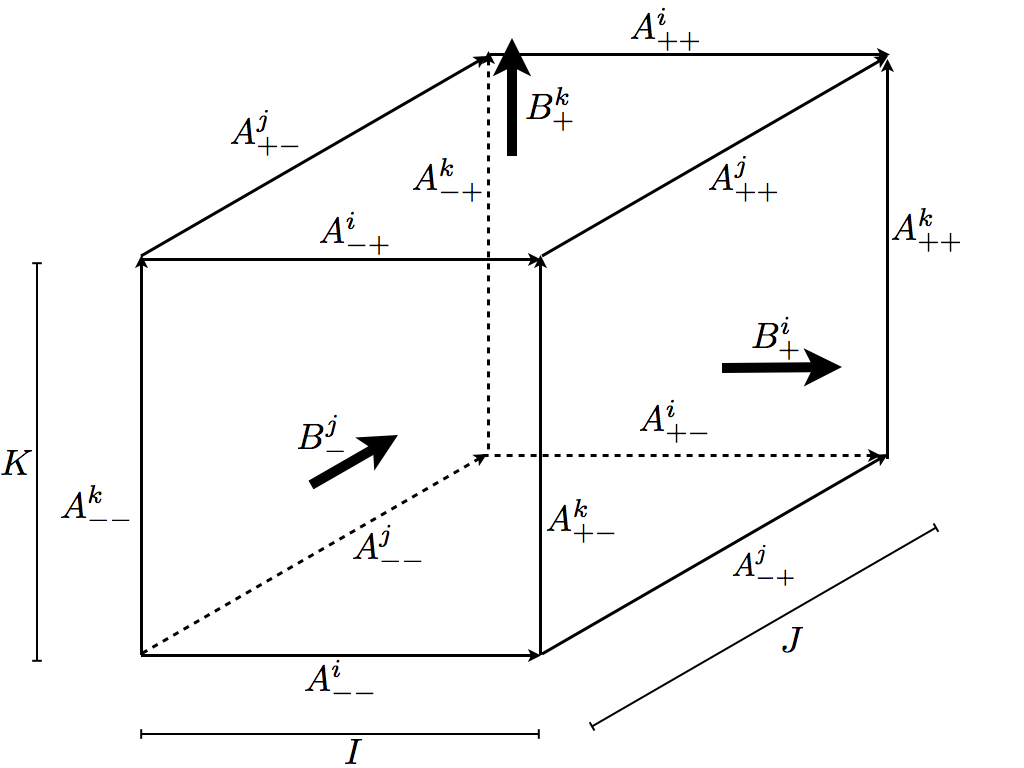
Figure 1: Example numerical grid cell, showing the locations at which various quantities are defined. Hydrodynamic quantities are defined at cell centers, magnetic fields at the centers of the cell faces (for clarity, only three of the six values for this cell are labeled), and magnetic vector potentials at the centers of cell edges. Due to the symmetry of the problem, $(i,j,k)$ may be taken as any positively oriented cycle of the elements $(x,y,z)$ See Eqs. (2), (4), and the surrounding text for an explanation of the index conventions for the fields.

We note that for the purposes of bookkeeping, the quantities defined above potentially have different dimensions because of the staggering. If the grid of cells has dimension $L\times M\times N$ in the $x$-, $y$-, and $z$-directions, respectively, then the numerical grid sizes of the magnetic quantities are as follows:

$$A^{x} :L\times(M+1)\times(N+1)\,, \quad B^{x} :(L+1)\times M\times N\,,$$

$$A^{y} :(L+1)\times M\times(N+1)\,, \quad B^{y} :L\times(M+1)\times N\,,$$

$$A^{z} :(L+1)\times(M+1)\times N\,, \quad B^{z} :L\times M\times(N+1)\,.$$ (7)

2.2 Uniqueness and gauge choice

Determining a vector potential $\mathbf{A}$ that corresponds to a given magnetic field $\mathbf{B}$ is an under-constrained problem, and solutions are never unique. This is known as the gauge freedom of $\mathbf{A}$. In general, if $\nabla\times\mathbf{A}=\mathbf{B}$, it is also true that

$$\nabla\times(\mathbf{A}+\nabla\phi)=\mathbf{B}\,,$$ (8)

for any scalar field $\phi$. For numerical reasons, the methods described here produce solutions in the Coulomb gauge, for which $\nabla\cdot\mathbf{A}=0$; i.e., the vector potential is also divergence-free. Numerically, this is equivalent to the condition

$$0= \left[\nabla\cdot\mathbf{A}\right](i+\nicefrac{{1}}{{2}},j+\nicefrac{{1}}{{2}},k+\nicefrac{{1}}{{2}})$$

$$= \frac{A^{x}(i+1,j+\nicefrac{{1}}{{2}},k+\nicefrac{{1}}{{2}})-A^{x}(i,j+\nicefrac{{1}}{{2}},k+\nicefrac{{1}}{{2}})}{I}$$

$$+\frac{A^{y}(i+\nicefrac{{1}}{{2}},j+1,k+\nicefrac{{1}}{{2}})-A^{y}(i+\nicefrac{{1}}{{2}},j,k+\nicefrac{{1}}{{2}})}{J}$$

$$+\frac{A^{z}(i+\nicefrac{{1}}{{2}},j+\nicefrac{{1}}{{2}},k+1)-A^{z}(i+\nicefrac{{1}}{{2}},j+\nicefrac{{1}}{{2}},k)}{K}\,,$$ (9)

where the natural location to evaluate this expression is at the grid vertices.

The Coulomb gauge is uniquely defined by requiring regularity when considering infinite domains. For finite domains, however, the Coulomb gauge solution is not unique, as one may add in gradients of the solutions of the Laplace equation that take the form $\mathbf{a}=\nabla(r^{l}Y_{lm})$, where $r$ is the spherical radius, $l$ is a non-negative integer, and $Y_{lm}$ is a spherical harmonic function, without affecting either the curl or the divergence of $\mathbf{A}$:

$$\nabla\times\mathbf{a}=\mathbf{0} \Rightarrow\nabla\times(\mathbf{A}+\mathbf{a})=\nabla\times\mathbf{A}=\mathbf{B}\,,$$

$$\nabla\cdot\mathbf{a}=0 \Rightarrow\nabla\cdot(\mathbf{A}+\mathbf{a})=\nabla\cdot\mathbf{A}=0\,.$$ (10)

Given that our domains are finite, we must therefore specify additional boundary conditions for our numerical solutions. These additional conditions are discussed below.

3 Solution techniques

In this section we describe two solution techniques to calculate the vector potential. We note that neither of these techniques are based on the Helmholtz decomposition, in which the vector potential can be calculated via:

$$\mathbf{A}_{\rm H}(\mathbf{r})=\frac{1}{4\pi}\int_{\mathcal{V}}\frac{\nabla^{\prime}\times\mathbf{B}(\mathbf{r}^{\prime})}{|\mathbf{r}-\mathbf{r}^{\prime}|}\mathrm{d}V^{\prime}-\frac{1}{4\pi}\oint_{\partial\mathcal{V}}\frac{\hat{\mathbf{n}}^{\prime}\times\mathbf{B}(\mathbf{r}^{\prime})}{|\mathbf{r}-\mathbf{r}^{\prime}|}\mathrm{d}S^{\prime}\,.$$ (11)

For magnetic fields that extend through the domain boundaries, the second term in this equation is a non-zero surface term that is more difficult to compute globally than either of the techniques we describe below. In addition, a corresponding expression for a scalar potential $\Phi$ includes an additional surface term that must be eliminated via a gauge transformation to obtain the correct vector potential. All in all, this is more work than our techniques.

3.1 Cell-by-cell generation of the vector potential

We present an algorithm for generating the vector potential on a cell-by-cell basis that is linearly dependent on the values of the magnetic field $\mathbf{B}$ across each face of the cell. The divergence of $\mathbf{B}$ is assumed numerically zero; if this isn’t the case—say because data were interpolated—we recommend use of a divergence cleaning method as a first step. Otherwise an inconsistent vector potential will be produced, as we define our staggered vector potential to produce a divergence-free magnetic field by construction.

The basic outline of the cell-by-cell method is as follows:

• Choose an arbitrary point on the grid to be the origin, and use the “six-face” technique (Sec. 3.1.1) to determine the $\mathbf{A}$-field values in that cell. For all our tests, we started in the corner of the grid for which $i=j=k=0$.

• Extend the solution along the six coordinate directions from the origin, using the “five-face” technique (Sec. 3.1.2) to incorporate the four previously determined values for the overlapping edges of the shared face.

• Further extend to the three “coordinate planes,” now using the “four-face” technique (Sec. 3.1.3) to take into account the seven previously computed edge values. (Note: If the chosen origin is (0,0,0), these planes would be the $xy$-, $xz$-, and $yz$-planes)

• Finish off the calculation by using the “three-face” technique (Sec. 3.1.4) on all remaining cells in the grid.

In Table 1, we list the number of times we use each of these techniques for a grid of size $L\times M\times N$, regardless of which cell is chosen to initiate the process.

Method	# of cells
Six-face	$1$
Five-face	$L+M+N-3$
Four-face	$LM+LN+MN-2(L+M+N)+3$
Three-face	$LMN-(LM+LN+MN)+(L+M+N)-1$

Table 1: Cell counts for each of the cell-by-cell techniques discussed below.

3.1.1 Initial cell: six undetermined faces

For the first cell in the grid that we consider, there is no prior information about the vector potential, and it must be completely determined based on the six values of the magnetic field across the faces. The problem is under-determined without making some assumptions. By assuming that whatever formulae we use to compute the vector potential will be invariant under rotations of the cube, we obtain a unique solution (as detailed in A):

$$A^{i}_{\scriptscriptstyle{--}} =\frac{5}{24}(-KB^{j}_{\scriptscriptstyle{-}}+JB^{k}_{\scriptscriptstyle{-}})+\frac{1}{24}(-KB^{j}_{\scriptscriptstyle{+}}+JB^{k}_{\scriptscriptstyle{+}})\,,$$

$$A^{i}_{\scriptscriptstyle{+-}} =\frac{5}{24}(-KB^{j}_{\scriptscriptstyle{+}}-JB^{k}_{\scriptscriptstyle{-}})+\frac{1}{24}(-KB^{j}_{\scriptscriptstyle{-}}-JB^{k}_{\scriptscriptstyle{+}})\,,$$

$$A^{i}_{\scriptscriptstyle{++}} =\frac{5}{24}(KB^{j}_{\scriptscriptstyle{+}}-JB^{k}_{\scriptscriptstyle{+}})+\frac{1}{24}(KB^{j}_{\scriptscriptstyle{-}}-JB^{k}_{\scriptscriptstyle{-}})\,,$$

$$A^{i}_{\scriptscriptstyle{-+}} =\frac{5}{24}(KB^{j}_{\scriptscriptstyle{-}}+JB^{k}_{\scriptscriptstyle{+}})+\frac{1}{24}(KB^{j}_{\scriptscriptstyle{+}}+JB^{k}_{\scriptscriptstyle{-}})\,,$$ (12)

where we may take any positive cyclic permutations of $x,y,z$ in terms of $i,j,k$.

3.1.2 Five undetermined faces

Once the vector potential is calculated for an initial cell, we may extend the solution to neighboring cells under the condition that the vector potential values shared with previously constructed cells are not changed.

As the solution is propagated in each coordinate direction from the initial cell, there will be cases in which one face and the four edges that surround it have already been determined, leaving five faces and eight edges yet to be determined. Call the previously determined face $B^{i}_{-}$, having denoted it $B^{i}_{+}$ when calculating vector potentials for the prior cell. For the new cell, we first compute a solution using the six-face technique described in Sec. 3.1.1, denoting it as $\tilde{A}$. In general this will lead to conflicting results for the previously determined overlapping edges because nothing enforces consistency between $\tilde{A}$ on our new cell compared to values from previous cells. To remove inconsistencies, we propagate changes to the non-overlapping, heretofore unspecified edges. To do so, we add a constraint based on consistency. If the six-face solution $\tilde{A}$ is consistent with previously computed values, we adopt it and move on. If not, we modify it on the eight undefined edges as follows.

Define $\hat{A}^{j}_{\pm-}$ and $A^{k}_{-\pm}$ to be the vector potential values computed previously for the face encompassing $B^{i}_{-}$, and define mismatches

$$\delta{A}^{j}_{\pm-}\equiv\tilde{A}^{j}_{\pm-}-\hat{A}^{j}_{\pm-}\,;~{}~{}\delta{A}^{k}_{-\pm}\equiv\tilde{A}^{k}_{-\pm}-\hat{A}^{k}_{-\pm}\,.$$ (13)

There are two consistent ways to determine the new edge values in a symmetric way (i.e. a way that is not preferential towards any one direction $x$, $y$, or $z$). The simplest is to propagate the differences from the edges surrounding the face $B^{i}_{-}$ to those surrounding the face $B^{i}_{+}$, making sure to keep the orientation of the change correct, setting

$$A^{j}_{\pm+} =\tilde{A}^{j}_{\pm+}-\delta A^{j}_{\pm-}\,,$$

$$A^{k}_{+\pm} =\tilde{A}^{k}_{+\pm}-\delta A^{k}_{-\pm}\,,$$

$$A^{i}_{\pm\pm} =\tilde{A}^{i}_{\pm\pm}\,.$$ (14)

Alternately, one may change the values of the terms $A^{i}_{\pm\pm}$ on the adjoining edges to the known face, leaving the edge values of the opposing face unchanged. We note that any linear combination of the two methods will also generate a consistent vector potential for the new cell as well. All results shown here use only the first of these methods.

3.1.3 Four undetermined faces

Once the solution for the vector potential has been extended in each cardinal direction from the initial cell, the next step is to expand it into the coordinate planes, the planes for which one index is equal to its “origin” value. If the chosen origin is (0,0,0), these planes would be the $xy$-, $xz$-, and $yz$-planes. This requires solving for the vector potential for cells in which edges for two adjoining faces have been determined, leaving five leftover edges spanning parts of the four remaining faces.

Again, we begin construction of the remaining vector potential values by using the six-face method to construct a set of values denoted $\tilde{A}$. If we assume that the faces containing the quantities $B^{i}_{\scriptscriptstyle{-}}$ and $B^{j}_{\scriptscriptstyle{-}}$ were previously determined, our task is to determine the new values for $A^{i}_{\scriptscriptstyle{+\pm}}$, $A^{j}_{\scriptscriptstyle{\pm+}}$, and $A^{k}_{\scriptscriptstyle{++}}$. The resulting problem is similar to the alternate approach for five undetermined faces, and we find

$$A^{i}_{\scriptscriptstyle{+-}} =\tilde{A}^{i}_{\scriptscriptstyle{+-}}-\frac{3\left(\delta A^{i}_{\scriptscriptstyle{--}}-\frac{I}{J}\delta A^{j}_{\scriptscriptstyle{--}}+\frac{I}{K}\delta A^{k}_{\scriptscriptstyle{-+}}\right)+\left(\delta A^{i}_{\scriptscriptstyle{-+}}-\frac{I}{J}\delta A^{j}_{\scriptscriptstyle{+-}}+\frac{I}{K}\delta A^{k}_{\scriptscriptstyle{+-}}\right)}{8}\,,$$

$$A^{j}_{\scriptscriptstyle{-+}} =\tilde{A}^{j}_{\scriptscriptstyle{-+}}-\frac{3\left(-\frac{J}{I}\delta A^{i}_{\scriptscriptstyle{--}}+\delta A^{j}_{\scriptscriptstyle{--}}+\frac{J}{K}\delta A^{k}_{\scriptscriptstyle{+-}}\right)+\left(-\frac{J}{I}\delta A^{i}_{\scriptscriptstyle{-+}}+\delta A^{j}_{\scriptscriptstyle{+-}}+\frac{J}{K}\delta A^{k}_{\scriptscriptstyle{-+}}\right)}{8}\,,$$

$$A^{i}_{\scriptscriptstyle{++}} =\tilde{A}^{i}_{\scriptscriptstyle{++}}-\frac{3\left(\delta A^{i}_{\scriptscriptstyle{-+}}-\frac{I}{J}\delta A^{j}_{\scriptscriptstyle{+-}}-\frac{I}{K}\delta A^{k}_{\scriptscriptstyle{-+}}\right)+\left(\delta A^{i}_{\scriptscriptstyle{--}}-\frac{I}{J}\delta A^{j}_{\scriptscriptstyle{--}}-\frac{I}{K}\delta A^{k}_{\scriptscriptstyle{+-}}\right)}{8}\,,$$

$$A^{j}_{\scriptscriptstyle{++}} =\tilde{A}^{j}_{\scriptscriptstyle{++}}-\frac{3\left(-\frac{J}{I}\delta A^{i}_{\scriptscriptstyle{-+}}+\delta A^{j}_{\scriptscriptstyle{+-}}-\frac{J}{K}\delta A^{k}_{\scriptscriptstyle{+-}}\right)+\left(-\frac{J}{I}\delta A^{i}_{\scriptscriptstyle{--}}+\delta A^{j}_{\scriptscriptstyle{--}}-\frac{J}{K}\delta A^{k}_{\scriptscriptstyle{-+}}\right)}{8}\,,$$

$$A^{k}_{\scriptscriptstyle{++}} =\tilde{A}^{k}_{\scriptscriptstyle{++}}\,.$$ (15)

Notice $A^{k}_{\scriptscriptstyle{++}}$ plays a slightly different role than the others as the edge bordering a pair of faces opposite the two has already been determined.

3.1.4 Three undetermined faces

The generic case describing the majority of the cells within our grid is one for which the vector potential has been determined on the nine edges encircling three adjoining faces of the cell. This leaves three undetermined edge values and three undetermined faces. If we assume that all data have been determined on the faces supplying the values for $B^{i}_{\scriptscriptstyle{-}}$, $B^{j}_{\scriptscriptstyle{-}}$, and $B^{k}_{\scriptscriptstyle{-}}$, then the only remaining vector potential values left to be determined would be $A^{i}_{\scriptscriptstyle{++}}$, $A^{j}_{\scriptscriptstyle{++}}$, and $A^{k}_{\scriptscriptstyle{++}}$. Once we have determined the value of any of these three, the other two values follow by requiring $\mathbf{B}=\nabla\times\mathbf{A}$ for each face. Once one of the three values is set, there is at most one undetermined edge on any face, so they can be easily calculated.

Using the same conventions as before, we may work out the values using our initial-cell techniques, defining differences as in the previous cases, and then evaluating the symmetric formulae

$$A^{i}_{\scriptscriptstyle{++}} =\tilde{A}^{i}_{\scriptscriptstyle{++}}-\frac{1}{3}\left(\delta A^{i}_{\scriptscriptstyle{+-}}+\delta A^{i}_{\scriptscriptstyle{-+}}-\frac{I}{J}\delta A^{j}_{\scriptscriptstyle{+-}}-\frac{I}{K}\delta A^{k}_{\scriptscriptstyle{-+}}\right)\,,$$

$$A^{j}_{\scriptscriptstyle{++}} =\tilde{A}^{j}_{\scriptscriptstyle{++}}-\frac{1}{3}\left(\delta A^{j}_{\scriptscriptstyle{+-}}+\delta A^{j}_{\scriptscriptstyle{-+}}-\frac{J}{K}\delta A^{k}_{\scriptscriptstyle{+-}}-\frac{J}{I}\delta A^{i}_{\scriptscriptstyle{-+}}\right)\,,$$

$$A^{k}_{\scriptscriptstyle{++}} =\tilde{A}^{k}_{\scriptscriptstyle{++}}-\frac{1}{3}\left(\delta A^{k}_{\scriptscriptstyle{+-}}+\delta A^{k}_{\scriptscriptstyle{-+}}-\frac{K}{I}\delta A^{i}_{\scriptscriptstyle{+-}}-\frac{K}{J}\delta A^{j}_{-+}\right)\,.$$ (16)

3.1.5 Conversion to Coulomb gauge and removal of noise

After applying this cell-by-cell algorithm, we find our solution to possess a few undesirable properties. First, nothing in these techniques will guarantee that the vector potentials we generate in a cell-by-cell way remain smooth, and indeed we find that by propagating changes across each cell in turn, we accrue rather large changes within a cell by the time we reach the edges of our grid, with potentially large jumps in the vector potential values on a cell-by-cell basis. Furthermore, the vector potential is determined in a gauge that seems arbitrary and has no convenient mathematical description. To minimize the first of these problems and eliminate the second, we convert our result to the Coulomb gauge using a convolution technique that is described below.

In general, our numerically constructed vector potential will not satisfy the Coulomb gauge condition. If we assume that we can determine a field $\phi$ to perform a gauge transformation of the form $\mathbf{A}_{C}=\mathbf{A}-\nabla\phi$, where $\mathbf{A}_{C}$ is our desired Coulomb gauge solution, under the condition that $\nabla\cdot\mathbf{A}_{C}=0$, we find

$$0=\nabla\cdot\mathbf{A}_{C} =\nabla\cdot\mathbf{A}-\nabla^{2}\phi$$

$$\nabla^{2}\phi =\nabla\cdot\mathbf{A}\,.$$ (17)

There are numerous ways to solve the resulting scalar Poisson equation, but given the absence of well-defined boundary conditions, we choose a Fast Fourier Transform (FFT)-based convolution method. Analytically, under the assumption that $\phi\to 0$ as $r\to\infty$, the solution to Eq. (17) is given by

$$\phi=-\frac{1}{4\pi}\iiint\frac{\left[\nabla\cdot\mathbf{A}\right](\mathbf{r}^{\prime})}{|\mathbf{r}-\mathbf{r}^{\prime}|}\mathrm{d}^{3}\mathbf{r}^{\prime}=\mathcal{F}^{-1}\left\{\mathcal{F}\left[\nabla\cdot\mathbf{A}\right]\star\mathcal{F}\left[-1/(4\pi r)\right]\right\}\,.$$ (18)

Here, the integral is evaluated over the volume of the computational domain, the symbols $\mathcal{F}$ and $\mathcal{F}^{-1}$ represent forward and reverse Fourier transforms respectively, and the $\star$ operator implies that the transformed arrays are multiplied element-by-element to perform a convolution. In practice, we do not actually convolve with the function $-1/4\pi r$ because it will not have zero Laplacian when discretized, yielding a solution that contains a nontrivial divergence. Instead, we numerically solve the three-dimensional Laplace equation for a $\delta$-function source and use this as a basis for our convolution kernel, as described in B.

3.2 Global linear algebra

Perhaps the most straightforward method to construct a staggered vector potential configuration corresponding to a given magnetic field is to treat the problem as a large, sparse linear algebra problem.

Let us first consider exactly how many equations need to be solved. According to Eq. (7), there are $3LMN+2(LM+LN+MN)+(L+M+N)$ vector potential values that must be set. Our direct cell-by-cell method yields a count for the number of equations that must be devoted to enforcing consistency between magnetic field values on cell faces and the vector potential values spanning that face. Noting that each “$n$”-face method provides $n-1$ consistency equations along with one that will automatically be satisfied by the divergence-free criterion, we find a total count of $2LMN+(LM+LN+MN)$ equations required to enforce consistency after summing over the cell counts shown in Table 1. To construct a well-posed system, the remaining equations, numbering $LMN+(LM+LN+MN)+L+M+N=(L+1)(M+1)(N+1)-1$ must be specified to choose a particular gauge condition. We note that this number corresponds to the total number of grid vertices present, save one.

While any gauge condition expressible in linear form may be chosen, we will describe how to implement the Coulomb gauge condition for the sake of consistency with the cell-by-cell method. For vertices on the interior of the grid, this simply means implementing Eq. (9), while for the vertices on the boundary we must make some assumption about the vector potential components that lie outside of the computational domain. We choose a simple, nonsingular option: zero the normal components of the vector potential at the boundary of the domain.

While it is straightforward to construct a sparse matrix problem whose solution is the desired vector potential configuration, computational efficiency concerns force us to consider the organization of the linear system. Unlike the case for calculating the convolution kernel for Coulomb gauge conversion described in Sec. 3.1.5, this matrix cannot be made diagonally dominant, nor can it easily be constructed in symmetric form, so several efficient techniques for solving sparse systems are immediately ruled out. We have found that most solvers perform better when the diagonal terms are non-zero in each row, and when the bandwidth of the non-zero elements is minimized, which motivates our approach to the problem. In what follows, we discuss a straightforward approach to generating a sparse linear system that yields a vector potential solution in the Coulomb gauge, satisfying the principles above.

Our linear system consists of one equation for each of the unknown vector potential values: a total of $3LMN+2(LM+LN+MN)+L+M+N$ equations. Each of the vector potential components is organized in dimension-by-dimension order, with the $z$-coordinate varying most rapidly and the $x$-coordinate the slowest. In order to maximize geometric proximity of neighboring elements in our linear system, we recommend interleaving the vector potential components; thus, successive rows of our matrix represent $A^{x}$, $A^{y}$, and $A^{z}$ components in turn (this is easiest for cubic grids, for which the different vector potential components contain the same number of elements on the grid).

The first set of linear equations is found by associating each $A^{x}$ value with a corresponding instance of the Coulomb gauge condition. In particular, the matrix row corresponding to a value $A^{x}(i,j+\nicefrac{{1}}{{2}},k+\nicefrac{{1}}{{2}})$ is associated with the equation

$$0=[\nabla\cdot\mathbf{A}](i+\nicefrac{{1}}{{2}},j+\nicefrac{{1}}{{2}},k+\nicefrac{{1}}{{2}})\,,$$ (19)

where the right-hand side is evaluated using Eq. (9). Again, any vector potential value lying outside the computational domain is set to zero. This has the effect of enforcing the Coulomb condition at every grid vertex in the domain except those on the “leftmost” face with coordinates $(-\nicefrac{{1}}{{2}},j+\nicefrac{{1}}{{2}},k+\nicefrac{{1}}{{2}})$, which are handled later.

For the rows corresponding to $A^{y}$ values, we use two different types of equations. For the leftmost set of values, i.e., those with $i=-\nicefrac{{1}}{{2}}$, the Coulomb condition is enforced, such that for the row corresponding to $A^{y}(-\nicefrac{{1}}{{2}},j,k+\nicefrac{{1}}{{2}})$, our matrix row implements the equation

$$0=[\nabla\cdot\mathbf{A}](-\nicefrac{{1}}{{2}},j+\nicefrac{{1}}{{2}},k+\nicefrac{{1}}{{2}})\,,$$ (20)

with the same treatment as above for components lying outside the computational domain. Combined with the previous step, the only vertices at which the Coulomb condition has not been applied are those on the grid edge satisfying the condition $i=j=-\nicefrac{{1}}{{2}}$.

For the remaining rows corresponding to $A^{y}$ values, we demand consistency with the $B^{z}$ value for the given magnetic field. In particular, for the row corresponding to $A^{y}(i+\nicefrac{{1}}{{2}},j,k+\nicefrac{{1}}{{2}})$, we implement the equation

$$B^{z}(i,j,k+\nicefrac{{1}}{{2}})= \frac{A^{y}(i+\nicefrac{{1}}{{2}},j,k+\nicefrac{{1}}{{2}})-A^{y}(i-\nicefrac{{1}}{{2}},j,k+\nicefrac{{1}}{{2}})}{I}$$

$$-\frac{A^{x}(i,j+\nicefrac{{1}}{{2}},k+\nicefrac{{1}}{{2}})-A^{x}(i,j-\nicefrac{{1}}{{2}},k+\nicefrac{{1}}{{2}})}{J}\,.$$ (21)

For rows corresponding to $A^{z}$ values, three sets of equations must be implemented:

1. For those on the edge of the domain, with coordinates $i=j=-\nicefrac{{1}}{{2}}$, the Coulomb gauge condition is applied, so that for the row corresponding to $A^{z}(-\nicefrac{{1}}{{2}},-\nicefrac{{1}}{{2}},k)$, we implement

   $$0=[\nabla\cdot\mathbf{A}](-\nicefrac{{1}}{{2}},-\nicefrac{{1}}{{2}},k+\nicefrac{{1}}{{2}})\,.$$ (22)

   At this point, the Coulomb condition has been enforced at every vertex within the domain, except the corner point with coordinates $i=j=k=-\nicefrac{{1}}{{2}}$. This serves as the single point at which we do not have the degrees of freedom available to implement the Coulomb condition.

2. For remaining $A^{z}$ values with coordinates $i=-\nicefrac{{1}}{{2}}$, we enforce consistency for given values of $B^{x}$. In particular, for rows corresponding to the values $A^{z}(-\nicefrac{{1}}{{2}},j+\nicefrac{{1}}{{2}},k)$, we implement

   $$B^{x}(-\nicefrac{{1}}{{2}},j,k)= \frac{A^{z}(-\nicefrac{{1}}{{2}},j+\nicefrac{{1}}{{2}},k)-A^{z}(-\nicefrac{{1}}{{2}},j-\nicefrac{{1}}{{2}},k)}{J}$$

   $$-\frac{A^{y}(-\nicefrac{{1}}{{2}},j,k+\nicefrac{{1}}{{2}})-A^{y}(-\nicefrac{{1}}{{2}},j,k-\nicefrac{{1}}{{2}})}{K}\,.$$ (23)

3. For the remaining rows corresponding to $A^{z}$ values lying elsewhere, with $i\neq-\nicefrac{{1}}{{2}}$, we enforce consistency for the given $B^{y}$ values. Rows corresponding to values $A^{z}(i+\nicefrac{{1}}{{2}},j+\nicefrac{{1}}{{2}},k)$ are used to solve the equations

   $$B^{y}(i,j+\nicefrac{{1}}{{2}},k)= \frac{A^{x}(i,j+\nicefrac{{1}}{{2}},k+\nicefrac{{1}}{{2}})-A^{x}(i,j+\nicefrac{{1}}{{2}},k-\nicefrac{{1}}{{2}})}{K}$$

   $$-\frac{A^{z}(i+\nicefrac{{1}}{{2}},j+\nicefrac{{1}}{{2}},k)-A^{z}(i-\nicefrac{{1}}{{2}},j+\nicefrac{{1}}{{2}},k)}{I}\,.$$ (24)

For input magnetic field configurations that are divergence-free, our method yields the unique vector potential consistent with both it as well as the gauge and boundary conditions. For a magnetic field that does contain numerical divergences, our method acts as an implicit one-dimensional “divergence cleaner”, sweeping numerical divergences off of the grid in a cell-by-cell fashion, working from the $B^{x}$ values on the leftmost face of the grid and transferring away divergences to the right and eventually out of the rightmost face of the grid. Our choice of the roles of the $x$-, $y$-, and $z$-directions is arbitrary, chosen simply for convenience.

The linear system of equations was implemented in the MUMPS [12, 13, 14] infrastructure, an MPI-parallelized sparse matrix package. With it, we are capable of generating suitable vector potentials even on numerical grids of order $100^{3}$ in size, as discussed and demonstrated in the following sections.

4 Code performance

We have tested the performance of our code on the NewHorizons computational cluster at RIT. Overall, it consists of 64-bit AMD and Intel CPUs interconnected with a high-speed, low-latency QDR InfiniBand fabric, and 4 GB of RAM per core. Specifically, our simulations were run on a subset of NewHorizons with dual-core AMD Opteron^TM processors.

Our cell-by-cell method is written as a serial code. As shown in Fig. 2, the computational time it requires scales linearly with the number of grid cells, and can be expected to follow this behavior even for much larger grids. Because the cell-by-cell method is strictly serial, it must be run on a single core, so the CPU core time is equal to the walltime. The code converges for all resolutions on a single core. It requires very little memory to generate its initial vector potential configuration beyond that required to store the magnetic field and vector potential values. Larger grids are required to perform the FFT convolution while converting the vector potential to the Coulomb gauge, but if need be this step could be separated from the rest of the code and run in parallel using the existing FFTW infrastructure [15], which is the leading MPI-parallelized multi-dimensional FFT package.

Fig. 3 shows that the walltime required to use our global linear algebra method largely scales as the number of gridpoints, $N$, to the $\nicefrac{{5}}{{3}}$ power, as expected due to how MUMPS implements basic Block-Low Rank (BLR) factorization [16]. The only significant deviation from this pattern appears at large grid sizes, for cases in which RAM runs out and swapping occurs. More minor deviations from this pattern occur due to matrix inversion requiring a significant communication overhead (handled internally by the MUMPS package). Thus the use of additional cores typically increases the required CPU core time to complete a run, even if walltime is reduced. In terms of memory, this method scales as $N$ to the $\nicefrac{{4}}{{3}}$ power.

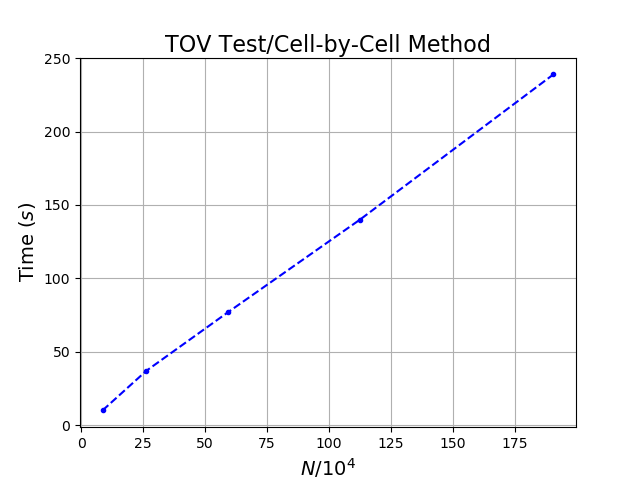
Figure 2: Scaling results for the cell-by-cell method, as measured in walltime versus number of grid cells.

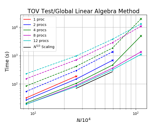
Figure 3: Walltime and CPU core time for the global linear algebra method run on different numbers of cores on NewHorizons. For a given number of CPU cores, the solid line represents the walltime, and the dashed line the CPU core time. Points marked with $\times$’s correspond to the highest resolution $N$ for which the code converges with the given amount of RAM (4GB/core on NewHorizons).

5 Numerical tests

To test our codes, we use the IllinoisGRMHD code within the Einstein Toolkit as our dynamical evolution code for various magnetized fluid configurations, as it evolves the magnetic vector potential over time as its dynamical variable. For each configuration, we perform the simulation twice.

First, we run IllinoisGRMHD to the designated final time as a baseline. We call this the “uninterrupted run”. Next we start a second, “restarted” run, in which the simulation proceeds to a predetermined “checkpoint” time, typically halfway through the simulation. At this point, we output the $\mathbf{A}$ field and numerically compute a $\mathbf{B}$ field from it (via the definition of $\mathbf{A}$) and use these magnetic fields as input for our cell-by-cell and global-linear-algebra codes. We then generate a new vector potential $\mathbf{A}^{\prime}$ from the $\mathbf{B}$ field, which will typically differ significantly from those generated by IllinoisGRMHD. We feed $\mathbf{A}^{\prime}$ back into IllinoisGRMHD and restart the run at the checkpoint time and continue until the final time.

We expect that if our approach is valid, the final magnetic fields (i.e., the physical, as opposed to the gauge-dependent, field) will agree to many significant digits between the restarted or uninterrupted runs. What follows is a demonstration of the validity of our approach in a variety of contexts: a magnetized two-dimensional, relativistically-spinning rotor (Sec. 5.1), a weakly-magnetized neutron star (Sec. 5.2.1), and an extremely-magnetized neutron star (Sec. 5.2.2).

5.1 Rotor test

The rotor test, as described in [17] consists of a disk of material in the $xy$-plane, referred to as a rotor, which possesses ten times the density of the surrounding material. The rotor is spinning such that its edge is moving at $0.995c$, and the entire medium is permeated by a uniform magnetic field in the $x$-direction. We run the simulations until the rotor has undergone two-thirds of a full rotation, with a checkpoint time ($t_{c}$) of one-third a full rotation.

Fig. 4 shows one component of the magnetic vector potential, $A^{x}$, in arbitrary units, plotted in the $xy$-plane at the checkpoint time. These are data from the output of the cell-by-cell method. Fig. 5 displays the magnetic field component $B^{x}$ on the same plane at the same time, also from the output of the cell-by-cell code. By inspection, these fields appear fairly smooth in their own right, but are they consistent with those of the uninterrupted run?

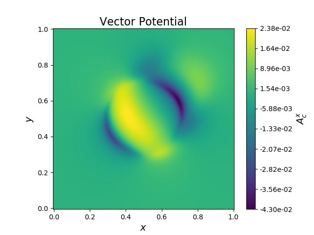
Figure 4: The magnetic vector potential $A^{x}$ plotted vs $x$ and $y$ at the checkpoint time $t_{c}$ after running through the cell-by-cell method. All quantities are in arbitrary units.

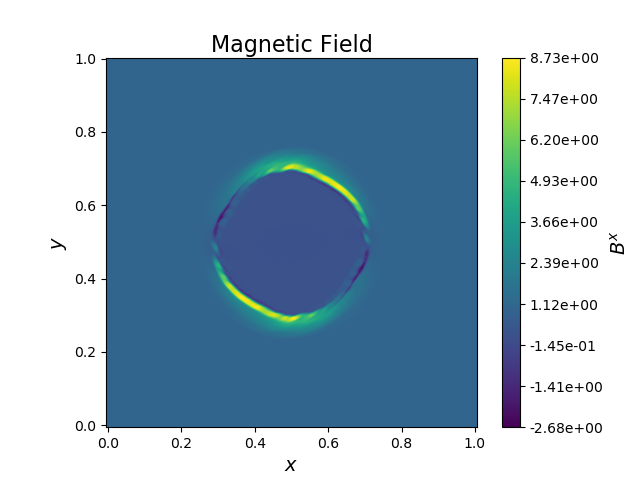
Figure 5: The magnetic field $B^{x}$ plotted vs $x$ and $y$ at the checkpoint time $t_{c}$ after running through the cell-by-cell method.

To compare the two runs of IllinoisGRMHD, we look at the components of the magnetic field $\mathbf{B}$. We do not directly compare the vector potential $\mathbf{A}$ between the two runs because the chosen vector potential gauges are different, depending both on whether an inverse curl algorithm is applied and on which such algorithm is chosen. Thus the final $\mathbf{A}$ field can be very different between uninterrupted and restarted runs, yet still yield the same magnetic field. This is why we say the magnetic field is the physically relevant quantity. Fig. 6 displays the dominant magnetic-field component, $B^{x}$, versus $x$ at the final time for all three runs: uninterrupted, restarted with cell-by-cell data, and restarted with global linear algebra data. Notice the agreement is within about one part in $10^{8}$ or more throughout the entire data set.

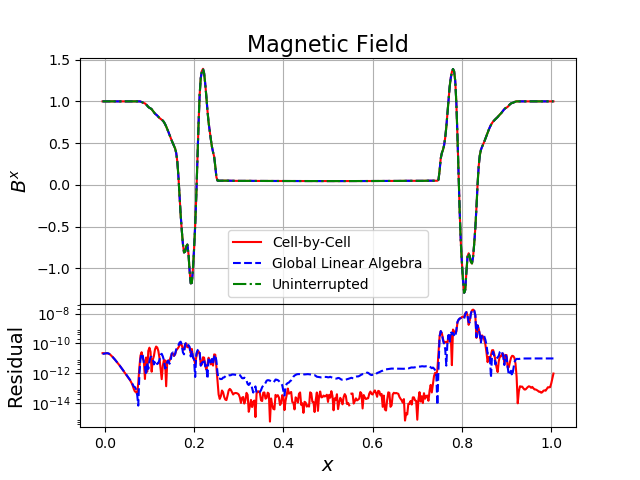
Figure 6: Top: The magnetic field $B^{x}$ vs $x$ at the final time $t_{f}$ after running the rotor through the cell-by-cell and global linear algebra methods. Bottom: The absolute difference between the cell-by-cell and global linear algebra runs and the corresponding uninterrupted run.

5.2 Magnetized neutron stars

Here we consider models of neutron stars with interior, poloidal magnetic fields, described using the Tolman-Oppenheimer-Volkhoff (TOV) model, a configuration that is also described in [17]. In Sec. 5.2.1, we start with a magnetic field strength parameter of $A_{b}\approx 0.64$, which results in a ratio of magnetic pressure to gas pressure of $b^{2}/2P\sim 0.001$. This should result in a star with little to no evolution due to magnetic effects, so we call this the “stable” case. Then, in Sec. 5.2.2, we set the initial magnetic field strength a value $10^{4}$ times larger, resulting in a magnetic to gas pressure ratio $10^{8}$ times larger. This should cause the magnetic pressure to violently blow apart the star, so we refer to this as the “unstable” case. The timescale of interest in these tests is the dynamical timescale of the stable TOV star, $t_{\rm dyn}$. The final time for all tests is fixed at $4\,t_{\rm dyn}$, and the checkpoint time is set to $t_{\rm dyn}$.

5.2.1 Magnetically stable case

As expected, there was not much evolution of the magnetic, hydrodynamic, or gravitational fields in the “stable” configuration. The neutron star slowly relaxes from its initial state. Fig. 7 shows the dominant magnetic field component ($B^{z}$) along the $x$ axis for the cell-by-cell and global linear algebra runs at the final time $4\,t_{\rm dyn}$. Conventions are the same as in Fig. 6. Agreement between runs is exceptional, particularly in the region of interest: the interior of the star ($|x|\lesssim 0.65$) where the magnetic fields remain nonzero throughout the evolution.

However, small disagreements exist at the boundary, due to the hybrid quadratic-cubic boundary conditions described in C. These boundary conditions pose some difficulty for numerical evolutions, as even the uninterrupted case shows the development of magnetic phenomena near the grid boundary. Also note this effect is only present on one side of the grid, when $x\approx-2$. We believe this to be due to IllinoisGRMHD’s extrapolation of $\mathbf{A}$ to fill in ghost cells at the boundary. In a full-scale simulation, the boundary will be sufficiently far away that such edge effects will not be a problem.

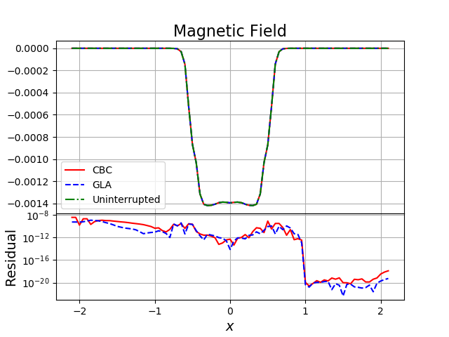
Figure 7: Top: The resultant $B^{z}$ vs $x$ after running the stable TOV star through the cell-by-cell and global linear algebra routines and restarting. Bottom: The absolute difference between the cell-by-cell and global linear algebra runs and the corresponding uninterrupted run. The checkpoint time was the dynamical time, and the final time was four times the dynamical time.

5.2.2 Magnetically unstable case

Our inverse curl algorithms also performed well in this test, though agreement dropped to about one part in $10^{4}$, likely due to the transmission of errors from the boundary (the simulation lasts $\approx 9$ light-crossing times). Over the course of the simulation, the star blew itself apart, ejecting material towards the edge of the grid. The data for $B^{z}$ vs $x$ are displayed in Fig. 8 using the same conventions as Fig. 7 in the previous section. Here the data on both ends of the grid ($x\approx-2$ and $x\approx 2$) actually match each other better than in the stable case. We think this is due to the behavior seen in the stable case being wiped out by the error caused by the outflow of the star exploding.

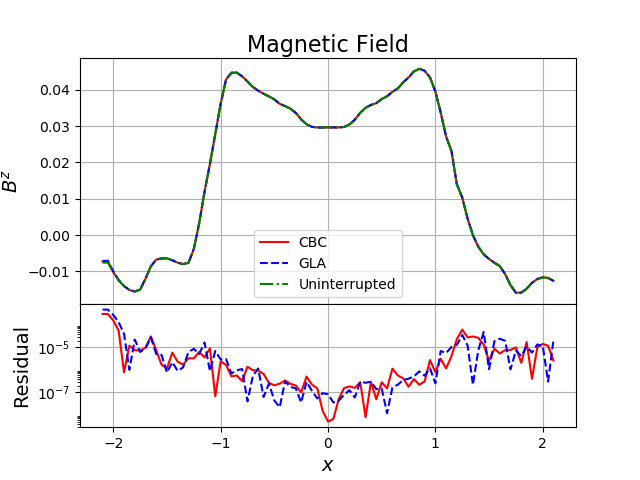
Figure 8: Top: The resultant $B^{z}$ vs $x$ after running the unstable TOV star through the cell-by-cell and global linear algebra routines and restarting. Bottom: The absolute difference between the cell-by-cell and global linear algebra runs and the corresponding uninterrupted run. The checkpoint time was the stable dynamical time, and the final time was four times the stable dynamical time.

6 Conclusion

The techniques described here are sufficient to construct a vector potential on a staggered numerical grid, appropriate for use in applications in which magnetic fields evolved using, e.g., a constrained transport approach, must be converted into a vector potential. Our solution consists of a numerical implementation of the “inverse curl” operator over a finite rectangular domain. This problem is typically much more difficult to solve than the case of a spherical domain, for which a spectral solution can be written down explicitly in terms of vector spherical harmonic modes. Additionally, these methods can be applied to any problem in which two quantities are related by the curl, such as the fluid velocity and vorticity in the context of fluid dynamics.

Each of our techniques possesses unique strengths and weaknesses. The cell-by-cell method is very fast and scales as $\mathcal{O}(N)$ in both time and memory. On the other hand, the global linear algebra method requires more memory and is slower, but it is a much more symmetric technique that uniformly cleans nonzero divergences in the input magnetic fields and applies Coulomb gauge conditions as it solves, instead of as a separate step. The global linear algebra method is also much more amenable to the implementation of different boundary conditions and mesh refinement than the cell-by-cell method.

Mesh refinement is an important tool used in numerical relativity simulations to apply additional resolution in regions where it is necessary, such as near black holes or neutron stars. Both Harm3D and IllinoisGRMHD have the capability to use mesh refinement, and so any method aimed at bridging the gap between them via inverse curl algorithms must also have such capabilities. Unfortunately, the staggering of the grid in the cell-by-cell method makes mesh refinement, even by a simple factor of two, prohibitively complicated and most likely infeasible. The global linear algebra method, however, can handle mesh refinement with careful consideration. Another way to implement mesh refinement is to use an inherently multi-grid method, which we explore in a upcoming paper.

Appendix A Notes on the direct cell-by-cell solution method

A.1 Six faces

To derive the “six-face” expressions for the vector potential values, a single configuration can be constructed to establish a maximally symmetric choice for the coefficients (i.e. a choice that is not preferential towards any one direction $x$, $y$, or $z$). In Fig. 9, a particular magnetic field configuration is shown, in which a magnetic field of magnitude $B^{k}_{\scriptscriptstyle{+}}=-4K$ can be seen as entering a cell from the top, while the values $B^{i}_{\scriptscriptstyle{\pm}}=\pm I,~{}B^{j}_{\scriptscriptstyle{\pm}}=\pm J$ represent the same field leaving the cell equally through the four sides. No flux enters or leaves through the bottom of the cell, where we set $B^{k}_{\scriptscriptstyle{-}}=0$. For this configuration, symmetry arguments can be used to specify each of the vector potential values. Around the top face of the cell, we expect the vector potential values to all be equal (up to a common scaling factor) depending on the dimensions of the cell:

$$A^{i}_{\scriptscriptstyle{++}}=-A^{i}_{\scriptscriptstyle{-+}}=JK\,;~{}~{}A^{j}_{\scriptscriptstyle{++}}=-A^{j}_{\scriptscriptstyle{+-}}=-IK\,,$$ (25)

while those on the bottom should all be zero:

$$A^{i}_{\scriptscriptstyle{\pm-}}=A^{j}_{\scriptscriptstyle{-\pm}}=0\,.$$ (26)

If we assume, based on the symmetry of the problem, that the vector potential on a given edge picks up a contribution proportional to a quantity $\alpha$ for the two faces that border the edge and a contribution $\beta$ from the two on the opposite sides from these, we find, for an edge value on the top face, that

$$A^{i}_{\scriptscriptstyle{++}} =\alpha(KB^{j}_{\scriptscriptstyle{+}}-JB^{k}_{\scriptscriptstyle{+}})+\beta(KB^{j}_{\scriptscriptstyle{-}}-JB^{k}_{\scriptscriptstyle{-}})\,,$$

$$JK =\alpha(5JK)-\beta(JK)~{}~{}\rightarrow~{}~{}5\alpha-\beta=1\,,$$ (27)

while for one on the bottom face,

$$A^{i}_{\scriptscriptstyle{--}} =\alpha(-KB^{j}_{\scriptscriptstyle{-}}+JB^{k}_{\scriptscriptstyle{+}})+\beta(-KB^{j}_{\scriptscriptstyle{+}}+JB^{k}_{\scriptscriptstyle{+}})\,,$$

$$0 =\alpha(JK)+\beta(-5JK)~{}~{}\rightarrow~{}~{}\alpha-5\beta=0\,.$$ (28)

The solution to this set of equations is $\alpha=5/24$, $\beta=1/24$.

This solution implies that for this configuration, the vertical edges, with values $A^{k}_{\pm\pm}$, which must be equal but could be assigned any value to yield a self-consistent magnetic field, will be set to zero. This seems appropriate, as it implies that for a spatially uniform magnetic field oriented along one of the coordinate axes, the vector potential values will be purely normal with no parallel component.

Figure 9: The sample configuration used to calculate $\alpha$ and $\beta$. This configuration is a magnetic field that enters the top of the box and uniformly leaves the sides. It results in the vector potential circulating around the four edges composing the top face, with the other eight vector potential values all evaluating to zero.

A.2 Five faces

When calculating the vector potentials for the five-face method, there are two independent methods by which differences may be symmetrically propagated between the previously calculated solution and the new six-face solution from the predetermined edges to those yet to be calculated. These differences may be computed in at least the following two ways:

• Propagate the differences from the face $B^{i}_{\scriptscriptstyle{-}}$ to $B^{i}_{\scriptscriptstyle{+}}$, making sure to keep the orientation of the change correct, using the result from Eq. (14).

• Change only the values of the terms $A^{i}_{\scriptscriptstyle{\pm\pm}}$ on the adjoining edges to the known face, leaving the edge values of the opposing face unchanged. The symmetric form of this operation is given by the set of equations:

  $$A^{i}_{\scriptscriptstyle{++}} =\tilde{A}_{\scriptscriptstyle{++}}-\frac{I\left[3(-K\delta A^{j}_{\scriptscriptstyle{+-}}-J\delta A^{k}_{\scriptscriptstyle{-+}})+(-K\delta A^{j}_{\scriptscriptstyle{--}}-J\delta A^{k}_{\scriptscriptstyle{--}})\right]}{8JK}\,,$$

  $$A^{i}_{\scriptscriptstyle{+-}} =\tilde{A}_{\scriptscriptstyle{-+}}-\frac{I\left[3(-K\delta A^{j}_{\scriptscriptstyle{--}}+J\delta A^{k}_{\scriptscriptstyle{-+}})+(-K\delta A^{j}_{\scriptscriptstyle{+-}}+J\delta A^{k}_{\scriptscriptstyle{--}})\right]}{8JK}\,,$$

  $$A^{i}_{\scriptscriptstyle{--}} =\tilde{A}_{\scriptscriptstyle{--}}-\frac{I\left[3(K\delta A^{j}_{\scriptscriptstyle{--}}+J\delta A^{k}_{\scriptscriptstyle{--}})+(K\delta A^{j}_{\scriptscriptstyle{+-}}+J\delta A^{k}_{\scriptscriptstyle{-+}})\right]}{8JK}\,,$$

  $$A^{i}_{\scriptscriptstyle{-+}} =\tilde{A}_{\scriptscriptstyle{+-}}-\frac{I\left[3(K\delta A^{j}_{\scriptscriptstyle{+-}}-J\delta A^{k}_{\scriptscriptstyle{--}})+(K\delta A^{j}_{\scriptscriptstyle{--}}-J\delta A^{k}_{\scriptscriptstyle{-+}})\right]}{8JK}\,,$$

  $$A^{j}_{\scriptscriptstyle{\pm+}} =\tilde{A}^{j}_{\scriptscriptstyle{\pm+}}\,,$$

  $$A^{k}_{\scriptscriptstyle{+\pm}} =\tilde{A}^{k}_{\scriptscriptstyle{+\pm}}\,,$$ (29)

  where the differences in the equations above are subject to a consistency condition:

  $$J(\delta A^{k}_{\scriptscriptstyle{-+}}-\delta A^{k}_{\scriptscriptstyle{--}})-K(\delta A^{j}_{\scriptscriptstyle{+-}}-\delta A^{j}_{\scriptscriptstyle{--}})=0\,.$$ (30)

We note that any linear combination of the two methods described above will also yield a valid solution.

Appendix B Convolution technique for Coulomb gauge condition

In what follows, we will simplify our discussion by assuming that our physical grid is cubic, with $N$ points in each dimension labeled from 1 to $N$, with uniform grid spacing $I$ in each of the three directions. We note, though, that these methods may be trivially generalized for cases where either the grid dimensions, grid spacings, or both are different in different directions.

In order to solve Eq. (18) via a convolution method, we will require a solution $\chi$ to the equation

$$\nabla^{2}\chi=\delta(r)\,,$$ (31)

which will serve as a convolution kernel. This kernel function must be evaluated on a grid at least one cell larger in each direction than our physical grid, indexed so that the origin is placed at a corner and the spatial domain is thought of as an octant. Thus we assume it is of size $N_{\rm ker}^{3}$, where $N_{\rm ker}\geq N+1$ and the indices run from 0 to $N_{\rm ker}-1$. Ideally, one should choose the value of $N_{\rm ker}$ to be the smallest allowed value that can be expressed in the form $2^{m}+1$, for positive integer $m$, or a similar quantity involving small-integer factors, in order to perform the FFT described below.

The analytic solution for Eq. (31) is well known to be $\chi=-1/4\pi r$, where $r$ is the three-dimensional distance from a point to the origin, $r(i,j,k)=I\sqrt{i^{2}+j^{2}+k^{2}}$, but this function $\chi$ is singular at the origin and not an exact solution if we interpret the Laplacian operator as a finite-differencing expression. Instead, we can solve

$$\chi^{*}(i-1,j,k) +\chi^{\prime}(i+1,j,k)+\chi^{*}(i,j-1,k)+\chi^{\prime}(i,j+1,k)$$

$$+\chi^{*}(i,j,k-1)+\chi^{\prime}(i,j,k+1)-6\chi(i,j,k)=\begin{cases}I^{2};&i=j=k=0\\ 0;&{\rm otherwise}\end{cases}\,,$$ (32)

where the notation $\chi^{*}$ is used to describe the appropriate boundary conditions that we will apply at the three faces of the cube describing coordinate planes, and the notation $\chi^{\prime}$ is used to describe those that we will apply at the three faces that lie on the exterior. At the former faces, we impose reflection symmetry, such that

$$\chi^{*}(i,j,k)=\begin{cases}\chi^{*}(1,j,k);&i=-1\\ \chi^{*}(i,1,k);&j=-1\\ \chi^{*}(i,j,1);&k=-1\\ \chi(i,j,k);&{\rm otherwise}\end{cases}\,,$$ (33)

in order to handle cases where a neighboring value lies outside the grid across one of the coordinate planes. At our outer boundaries, we impose a $1/r$ falloff condition:

$$\chi^{\prime}(i,j,k)=\begin{cases}\frac{r(N_{\rm ker}-1,j,k)}{r(N_{\rm ker},j,k)}\chi^{\prime}(N_{\rm ker}-1,j,k);&i=N_{\rm ker}\\ \\ \frac{r(i,N_{\rm ker}-1,k)}{r(i,N_{\rm ker},k)}\chi^{\prime}(i,N_{\rm ker}-1,k);&j=N_{\rm ker}\\ \\ \frac{r(i,j,N_{\rm ker}-1)}{r(i,j,N_{\rm ker})}\chi^{\prime}(i,j,N_{\rm ker}-1);&k=N_{\rm ker}\\ \\ \chi(i,j,k);&{\rm otherwise}\end{cases}\,,$$ (34)

though the Dirichlet condition $\chi^{\prime}(i,j,k)=0$ would also be a valid choice. The resulting linear system, which is sparse and diagonally dominant, can be solved using any standard linear algebra package. We have done so using eigen [18].

To perform the FFT-based convolution, we need to map the convolution kernel function and the grid containing the divergence of the vector potential into a larger grid, to avoid aliasing effects. Assuming that we have chosen the value of $N_{\rm ker}$ appropriately, our FFT grids will have dimensions $N_{\rm fft}\times N_{\rm fft}\times N_{\rm fft}$, where $N_{\rm fft}=2(N_{\rm ker}-1)$ and we assume the indices range from 0 to $N_{\rm fft}-1$ in each direction. The convolution kernel function is

$$\chi_{\rm fft}(i,j,k)=\chi(I,J,K)\,,$$ (35)

where $I=\min(i,N_{\rm fft}-i)$, $J=\min(j,N_{\rm fft}-j)$, and $K=\min(k,N_{\rm fft}-k)$. The data array is given by

$$\psi_{\rm fft}(i,j,k)=\begin{cases}\left[\nabla\cdot\mathbf{A}\right](i-\nicefrac{{1}}{{2}},j-\nicefrac{{1}}{{2}},k-\nicefrac{{1}}{{2}});&i<N~{}{\rm and}~{}j<N~{}{\rm and}~{}k<N\\ 0;&{\rm otherwise}\end{cases}\,.$$

We may now evaluate

$$\phi_{\rm fft}=\mathcal{F}^{-1}\left\{\mathcal{F}[\psi_{\rm fft}]\star\mathcal{F}[\chi_{\rm fft}]\right\}\,,$$ (36)

where the symbols $\mathcal{F}$ and $\mathcal{F}^{-1}$ represent forward and reverse Fourier transforms, and the $\star$ operator implies that we multiply the transformed arrays against each other element by element. Our implementation uses the FFTW package to perform these operations. Having calculated this field, we may then set

$$\phi(i-\nicefrac{{1}}{{2}},j-\nicefrac{{1}}{{2}},k-\nicefrac{{1}}{{2}})=\phi_{\rm fft}(i,j,k)\,,$$ (37)

for all indices $1\leq i\leq N$, $1\leq j\leq N$, and $1\leq k\leq N$ and then set $\mathbf{A}_{c}=\mathbf{A}-\nabla\phi$ using our staggered coordinates, e.g.,

$$A_{c}^{x}(i,j+\nicefrac{{1}}{{2}},k+\nicefrac{{1}}{{2}})= A^{x}(i,j+\nicefrac{{1}}{{2}},k+\nicefrac{{1}}{{2}})$$

$$-\frac{\phi(i+\nicefrac{{1}}{{2}},j+\nicefrac{{1}}{{2}},k+\nicefrac{{1}}{{2}})-\phi(i-\nicefrac{{1}}{{2}},j+\nicefrac{{1}}{{2}},k+\nicefrac{{1}}{{2}})}{I}\,.$$ (38)

The resulting vector potential configuration satisfies the Coulomb condition in the interior and remains consistent with the given magnetic field, both up to machine precision levels everywhere.

Appendix C Ghost cell treatment

IllinoisGRMHD explicitly creates ghost cells outside the grid. However, the cell-by-cell and global linear algebra methods do not take this into account. They treat all the data as if they are part of the physical grid. Without any adjustment, this causes inconsistencies when data are fed back into IllinoisGRMHD because by default, IllinoisGRMHD linearly extrapolates data in the ghost cells. This is an issue outside of the $\mathbf{B}$ to $\mathbf{A}$ calculation; it is purely related to the interface with IllinoisGRMHD. Therefore it is valid to handle the ghost cells independent of the $\mathbf{B}$ to $\mathbf{A}$ calculation.

To achieve matching behavior at the boundaries between our methods and IllinoisGRMHD, it is necessary to treat different ghost zones in different ways. This is due to staggering of the data in our methods and IllinoisGRMHD, as described in Section 2. If we just extrapolated all $\mathbf{A}$-values linearly to match the IllinoisGRMHD default, we would introduce errors into the condition that $\mathbf{B}=\nabla\times\mathbf{A}$. Therefore we use hybrid quadratic-cubic conditions. In this scheme, ghost values are handled as follows: normal $\mathbf{A}$-field components are extrapolated quadratically from data within the physical grid, and tangential $\mathbf{A}$-field components are extrapolated cubically.

For example, if we are looking at the ghost cells on the $+x$-side of the grid, then we would have

$$A^{x}(i,j,k)= 3A^{x}(i-1,j,k)-3A^{x}(i-2,j,k)+A^{x}(i-3,j,k)$$

$$A^{y}(i,j,k)= 4A^{y}(i-1,j,k)-6A^{y}(i-2,j,k)+4A^{y}(i-3,j,k)$$

$$-A^{y}(i-4,j,k)$$

$$A^{z}(i,j,k)= 4A^{z}(i-1,j,k)-6A^{z}(i-2,j,k)+4A^{z}(i-3,j,k)$$

$$-A^{z}(i-4,j,k)\,,$$ (39)

where, if the number of ghost cells on either side of the grid is $n_{\mathrm{ghost}}$, $i$ runs from $L+n_{\mathrm{ghost}}-1$ to $L+2(n_{\mathrm{ghost}}-1)$, inclusive, and $j$ and $k$ cover their full range of values, including ghost cells.

References

References

- [1] D. S. Balsara, D. S. Spicer, A Staggered Mesh Algorithm Using High Order Godunov Fluxes to Ensure Solenoidal Magnetic Fields in Magnetohydrodynamic Simulations, J. Comp. Phys. 149 (1999) 270–292. doi:10.1006/jcph.1998.6153.
- [2] G. Tóth, The Constraint in Shock-Capturing Magnetohydrodynamics Codes, J. Comp. Phys. 161 (2000) 605–652. doi:10.1006/jcph.2000.6519.
- [3] Z. B. Etienne, V. Paschalidis, R. Haas, P. Mösta, S. L. Shapiro, IllinoisGRMHD: an open-source, user-friendly GRMHD code for dynamical spacetimes, Classical and Quantum Gravity 32 (17) (2015) 175009. arXiv:1501.07276, doi:10.1088/0264-9381/32/17/175009.
- [4] C. F. Gammie, J. C. McKinney, G. Tóth, HARM: A Numerical scheme for general relativistic magnetohydrodynamics, Astrophys. J. 589 (2003) 444–457. arXiv:astro-ph/0301509, doi:10.1086/374594.
- [5] S. Sahoo, Inverse Vector Operators, ArXiv e-printsarXiv:0804.2239.
- [6] G. M. Webb, Q. Hu, B. Dasgupta, G. P. Zank, Homotopy formulas for the magnetic vector potential and magnetic helicity: The Parker spiral interplanetary magnetic field and magnetic flux ropes, Journal of Geophysical Research (Space Physics) 115 (2010) 10112. doi:10.1029/2010JA015513.
- [7] K. T. Edler, Spherical harmonic inductive detection coils and their use in dynamic pre-emphasis for magnetic resonance imaging, Ph.D. thesis, University of Manitoba (Canada) (2010).
- [8] S. Yang, J. Büchner, J. Carlo Santos, H. Zhang, Method of Relative Magnetic Helicity Computation II: Boundary Conditions for the Vector Potentials, ArXiv e-printsarXiv:1304.3526.
- [9] N. Demerdash, T. Nehl, F. Fouad, Finite element formulation and analysis of three dimensional magnetic field problems, IEEE Transactions on Magnetics 16 (1980) 1092–1094. doi:10.1109/TMAG.1980.1060817.
- [10] O. Biro, K. Preis, K. R. Richter, On the use of the magnetic vector potential in the nodal and edge finite element analysis of 3D magnetostatic problems, IEEE Transactions on Magnetics 32 (1996) 651–654. doi:10.1109/20.497322.
-
[11]
GitHub repository containing
our methods.
URL https://github.com/zsilberman/Inverse-Curl -
[12]
P. R. Amestoy, I. S. Duff, J.-Y. L’Excellent, J. Koster,
A fully asynchronous
multifrontal solver using distributed dynamic scheduling, SIAM Journal on
Matrix Analysis and Applications 23 (1) (2001) 15–41.
doi:10.1137/S0895479899358194.
URL https://doi.org/10.1137/S0895479899358194 - [13] P. R. Amestoy, A. Guermouche, J.-Y. L’Excellent, S. Pralet, Hybrid scheduling for the parallel solution of linear systems, Parallel Computing 32 (2) (2006) 136 – 156, parallel Matrix Algorithms and Applications (PMAA’04). doi:https://doi.org/10.1016/j.parco.2005.07.004.
-
[14]
MUMPS: A Parallel Sparse
Direct Solver.
URL http://mumps.enseeiht.fr/index.php?page=home - [15] M. Frigo, S. G. Johnson, The design and implementation of FFTW3, Proceedings of the IEEE 93 (2) (2005) 216–231, special issue on “Program Generation, Optimization, and Platform Adaptation”.
- [16] P. Amestoy, A. Buttari, J.-Y. L’Excellent, T. Mary, On the complexity of the block low-rank multifrontal factorization, SIAM Journal on Scientific Computing 39 (4) (2017) A1710–A1740. arXiv:https://doi.org/10.1137/16M1077192, doi:10.1137/16M1077192.
- [17] P. Mösta, B. C. Mundim, J. A. Faber, R. Haas, S. C. Noble, T. Bode, F. Löffler, C. D. Ott, C. Reisswig, E. Schnetter, GRHydro: a new open-source general-relativistic magnetohydrodynamics code for the Einstein toolkit, Classical and Quantum Gravity 31 (1) (2014) 015005. arXiv:1304.5544, doi:10.1088/0264-9381/31/1/015005.
-
[18]
G. Guennebaud, B. Jacob, et al., Eigen v3
(2010).
URL http://eigen.tuxfamily.org