Massively parallel simulations of binary black holes with Dendro-GR

Abstract

We present results from the new Dendro-GR code. These include simulations of binary black hole mergers for mass ratios up to $q=16$. Dendro-GR uses Wavelet Adaptive Multi-Resolution (WAMR) to generate an unstructured grid adapted to the spacetime geometry together with an octree based data structure. We demonstrate good scaling, improved convergence properties and efficient use of computational resources. We validate the code with comparisons to LazEv.

I Introduction

The gravitational wave detectors LIGO/Virgo have made a number of epochal discoveries [1, 2]. These have given us a dramatically broader conception and understanding of the high-energy universe and some of its compact object constituents [3, 4, 5] As these detectors continually improve [6, 7, 8] and are added to by new detectors, such as KAGRA [9], we can confidently expect an ongoing parade of additional discoveries.

The detection and analysis of gravitational waves uses a library of modeled waveforms for comparison with the detector output signal. Numerical relativity waveforms are computed using the full nonlinear, Einstein equations, and these waveforms span the evolution of the binary system from inspiral, through merger, and finally to ringdown. These waveforms may be used directly in the analysis of gravitational waves [10, 11], or to inform and validate faster, approximate methods for generating waveforms, such as semi-analytical and phenomenological methods (see, e.g., [12, 13, 14, 15, 16, 17, 18, 19]). Numerical relativity can also probe certain astrophysical scenarios that are difficult to model with approximate methods. Examples of such scenarios include non-vacuum spacetimes, such as systems with neutron stars, accretion disks, and/or magnetic fields. Even some vacuum binary black hole systems can be difficult to model with approximate techniques, such as binaries with large eccentricity, high spins, or large mass ratios. We use the mass ratio $q=m_{1}/m_{2}$, where $m_{1}$ is the mass of the primary with $m_{1}\geq m_{2}$.

While there are advantages to using numerical relativity waveforms directly in gravitational wave analysis, there are significant challenges in calculating waveforms of sufficient quality. The waveforms must be sufficiently long, have errors bounded within known tolerances, and they must span a large region of the binary parameter space. The development of newer, more sensitive gravitational wave detectors significantly complicates the challenge. For example, recent work on requirements for third generation detectors [20, 21, 22] and LISA [23] estimate that errors in numerical relativity waveforms need to be reduced by an order of magnitude [24]. Another study found that numerical resolutions of BBH spacetimes will need to be increased by almost a factor of ten in some cases [25]. Reducing the error in numerical waveforms to the level required by 3G detectors will require new algorithms and methods in numerical relativity.

The challenge of producing waveforms for future gravitational wave detectors will require highly scalable numerical relativity codes that are able to efficiently run on exascale supercomputers. Dendro-GR is a new code for relativistic astrophysics that is designed to meet some of the next-generation challenges in numerical relativity. Dendro-GR scales well on massively parallel supercomputers, and it uses fast, responsive adaptive multi-resolution based on wavelets (WAMR). Importantly, Dendro-GR easily accommodates many well-tested numerical methods that have been developed in the relativity community, such as the evolution of Einstein equations in the BSSN formalism and high-resolution shock-capturing methods for relativistic fluid dynamics.

Several projects are currently being developed in the community that use modern adaptive-mesh infrastructures and sophisticated numerical algorithms to meet this computational challenge. Among these are GR-Athena++ [26], which uses the highly-efficient octree AMR infrastructure of Athena++ for full numerical relativity simulations coupled to GRMHD, GR-Chombo [27], a fully modern AMR numerical relativity code allowing for complex grid configurations, and CarpetX, which is a new AMR driver for the Einstein Toolkit [28, 29] that is built on the AMReX toolkit [30]. Pseudospectral and discontinuous Galerkin methods promise some advantages for massively parallel computing. Spectre [31] uses discontinuous Galerkin methods and a task-based parallelization scheme. Nmesh [32, 33] and bamps [34] are other codes using DG methods. Simflowny [35] has a domain specific language and a web-based development environment and graphical user interface. Simflowny can generate code for multiple platforms, such as SAMRAI [36]. Dendro-GR uses an efficient octree structure to store the grid elements similar in spirit to that used in GR-Athena++. While Dendro-GR’s wavelet decomposition with an unstructured grid is similar in spirit to Spectre.

This paper presents results from some of the first binary black hole mergers performed with Dendro-GR. We study gravitational waves from binary black hole systems with mass ratios up to $q=16$. We compare results with the well-known LazEv [37, 38] code in some cases, and find that the solutions match in the convergence limit. We also present performance data for Dendro-GR.

II Methods

Dendro-GR has been built with the intention of tackling relativistic astrophysics problems involving merging compact objects. Its development uses and accommodates a number of standard techniques within numerical relativity as well as including some new approaches; all with an eye to improving the efficiency, scalability and time to solution for still challenging problems such as large mass ratio binary black holes. Among the conventional and well-tested numerical methods used in Dendro-GR   we solve the Einstein equations using the BSSN formulation together with typical coordinate conditions, initial data, and finite differencing algorithms. Newer approaches used within Dendro-GR include some of the following and are discussed at greater length subsequently in this section. The code uses a dynamic grid which is constructed via an expansion of the grid functions in an interpolating wavelet basis. In this basis, terms in the wavelet expansion can be mapped to individual grid points. The resulting unstructured grid is naturally represented computationally as an octree. On integrating the equations of motion in time, each node of this octree is separately unzipped (decompressed) into a local point representation on a uniform Cartesian grid. The integrated functions are then zipped (compressed) back to a sparse representation by thresholding the coefficients of the wavelet expansion. This sparse representation is compact and computationally efficient as it conserves computer memory and reduces parallel communication. This section describes some of these key components of Dendro-GR in more detail. We begin with a brief description of our formalism for solving the Einstein equations and setting initial data. We then describe the generation of the grid using WAMR and the process for integrating the equations.

II.1 Formalism

There is an extensive literature on solving the BSSN equations in general relativity, including monographs such as [39, 40, 41, 42]. This section briefly outlines our particular choices for solving the BSSN equations. We write the BSSN equations in terms of the conformal factor [38]

$$\chi^{-1}=\det(\gamma_{ij}).$$ (1)

For gauge conditions, we use the “$1+\log$” slicing condition and the $\Gamma$-driver shift as used in [43]

$$\partial_{t}\alpha = \beta^{i}\partial_{i}\alpha-2\alpha K$$ (2)

$$\partial_{t}\beta^{i} = \beta^{j}\partial_{j}\beta^{i}+{3\over 4}B^{i}$$ (3)

$$\partial_{t}B^{i} = \beta^{j}\partial_{j}B^{i}+\partial_{t}{\tilde{\Gamma}}^{i}-\beta^{j}\partial_{j}{\tilde{\Gamma}}^{i}-\eta B^{i}.$$ (4)

Spatial derivatives are calculated using centered finite difference operators that are ${\rm O}(h^{6})$ in the grid spacing, $h$.

The semi-discrete Einstein equations are integrated in time using explicit fourth-order Runge-Kutta and a CFL of 0.25. Kreiss-Oliger dissipation is added to the equations using a fifth-order operator

$$\Delta^{6}_{x}u^{n}_{m} =\left(-u^{n}_{m+3}+6u^{n}_{m+2}-15u^{n}_{m+1}+20u^{n}_{m}\right.$$

$$\quad\left.-15u^{n}_{m+1}+6u^{n}_{m-2}-u^{n}_{m-3}\right)/\left({64\triangle x}\right),$$ (5)

with a tunable amplitude parameter $\sigma$, $0\leq\sigma<1$, which allows one to adjust the amount of dissipation [39]. As discussed below in Section IV.1, we found best results with $\sigma=0.4$. We make the common choice to enforce certain algebraic constraints and derivative definitions as described, for example, in [44]. Outgoing radiative boundary conditions are applied to the dynamical variables.

We extract gravitational waves from our simulations at five radii between $50\>M\leq r\leq 100\>M$ using the Penrose scalar, $\psi_{4}$ [39, 45]. Their decomposition with respect to spin weighted spherical harmonics (SWSH) is performed using Lebedev quadrature [46]. To evaluate $\psi_{4}$ at each of the quadrature points on each 2-sphere, we perform an efficient search operation on the underlying grid, and SWSH projection coefficients are computed with a parallel reduction operation [47].

II.2 Initial Data

Initial data for both Dendro-GR and LazEv are set using the TwoPunctures code [48] from the EinsteinToolkit [29, 28]. For the initial values of shift, both codes set $\beta^{i}(t=0)=0$. Initial values of the lapse in Dendro-GR  use the ad-hoc function $\alpha(t=0)=\tilde{\psi}^{-2}$, where $\tilde{\psi}=1+m_{p1}/(2r_{1})+{m}_{p2}/(2r_{2})$, $r_{i}$ is the coordinate distance to the $i$th BH, and ${m}_{pi}$ is the bare mass parameter of the $i$th BH. In LazEv   the initial lapse is $\tilde{\psi}=1+1/(4r_{1})+1/(4r_{2})$.

Table 1: The initial configuration parameters for non-spinning binary black hole systems for increasing mass ratio. The presented numerical waveforms are based on these initial data parameters. The parameters for $q\geq 2$ were obtained using the expressions in [49]. The initial data are set using the bare mass parameters. The black holes are placed initially on the $x$-axis at the locations $x_{1}$ and $x_{2}$ as given in the table. The linear momentum of the the second black hole is given in the last two columns, $\mathbf{p}_{2}=(p_{x},p_{y})$, and $\mathbf{p}_{1}=-\mathbf{p}_{2}$.

Mass ratio	Puncture Parameter		ADM Mass		Total	x-position		Momentum BH2
$q=m_{1}/m_{2}$	$m_{p2}$	$m_{p1}$	$m_{2}$	$m_{1}$	ADM Mass	$x_{2}$	$x_{1}$	$p_{x}$	$p_{y}$
1	4.8240E-1	4.8240E-1	5.0010E-1	5.0010E-1	9.8844E-1	4	-4	0	0.1140
2	0.31715	0.65150	6.6667E-1	-3.3333E-1	9.8931E-1	5.3238	-2.6762	-1.7777E-03	1.0049E-01
4	1.8805E-01	7.8937E-01	2.0000E-1	8.0000E-1	9.9237E-1	6.3873	-1.6127	-1.0647E-03	7.2660E-02
8	1.0362E-01	8.8245E-01	1.1111E-1	8.8889E-1	9.9534E-1	7.1006	-8.9938E-1	-4.9937E-04	4.5037E-02
16	5.4585E-02	9.3761E-01	5.8824E-2	9.4118E-1	9.9740E-1	7.5226	-4.7741E-1	-1.9532E-04	2.5319E-02

In this paper, we evolve non-spinning black hole binaries with mass ratios $q=1,2,4,8$, and $16$. We place the black holes initially on the $x$-axis, with the binary’s center of mass at the origin. The smaller black hole with mass $m_{2}$ is placed on the positive $x$-axis, and the initial coordinate separation is fixed to $x_{2}-x_{1}=8\>M$. Initial data parameters for the $q=1$ binary are ad-hoc quasi-circular parameters, chosen to match previous work [50]. Parameters for all other cases were found using the low eccentricity post-Newtonian expressions reported in [49]. To simplify comparisons with LazEv, we set the TwoPunctures code to use the bare puncture masses and other parameters shown in Table 1 directly. Finally, we ran the $q=1,2$, and $4$ cases with both Dendro-GR and LazEv, while the higher mass ratio simulations were only run with Dendro-GR.

II.3 Symbolic code generation

The evaluation of the BSSN equations at a given grid point is computationally expensive and can be challenging due to the large number of terms associated with the equations. Manually writing code to evaluate these equations can be prone to error, difficult to debug, and challenging to perform architecture specific optimizations. To address some of these issues, we have developed a SymPy-based code generation framework for Dendro-GR. This tool has some of the same capabilities as NrPy+ [51, 52], but is more limited in scope. Using our symbolic framework, we compute the directed acyclic graph representing the underlying computations for the BSSN equations. We perform optimizations to reduce the overall number of operations as well as architecture specific optimizations that improve our code’s performance portability. The current implementation of the symbolic framework supports CPUs and GPUs [53, 47].

II.4 Grid generation with WAMR

The computational complexity of the Einstein equations, together with the requirement of high accuracy across multiple spatial and temporal scales, motivates the use of grid adaptivity. Dendro-GR uses a wavelet-based approach which results in a representation of the underlying field variables on a sparse, adaptive mesh. We describe briefly here the fundamental aspects of this sparse representation. More complete details can be found in [54, 55, 47, 53]. While we use the coefficients in a wavelet expansion to generate the computational grid, we store the grid functions only in the point representation. Thus, the wavelet coefficients are not used to integrate the equations of motion.

Two essential ingredients in our approach are the notion of iterative interpolation [56] and the wavelet representation itself [57, 58]. We demonstrate both of these in one dimension. The extension to multiple dimensions is straightforward and is accomplished by simply repeating the procedures we will describe in each additional dimension. To fix ideas, we first define a set of nested grids, $V_{j}$, where

$$V_{j}=\bigl{\{}x^{j,k}:x^{j,k}=2^{-j}\,k\Delta x\bigr{\}},$$

where $j$ and $k$ are nonnegative integers and $\Delta x$ is the spacing on the base grid (or level) and which is labeled with $j=0$. This base grid, $V_{0}$, is comprised of $N+1$ gridpoints evenly spaced on a domain of length $L=N\Delta x$. Each finer grid with $j>0$ contains each point in every coarser grid. Values of a field, $u$, at level $j$ are designated $u(x^{j,k})\equiv u^{j,k}$. If known, these values are copied from coarser grids to all required fine grids. For example to go from $V_{j}$ to $V_{j+1}$, we take $u^{j+1,2k}=u^{j,k}$. A similar copy happens to all higher level fine grids. Of course, on these finer grids, there will be points newly appearing. The field values on those gridpoints new to grid $V_{j+1}$ are interpolated from the known values on the coarser grid $V_{j}$. We generally use Lagrange interpolation. In this manner, all fields at any refinement level can be had (see Fig. 2). This iterated interpolation, continued to arbitrarily large levels produces continuous functions with compact support [57].

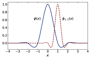
Figure 1: This shows the fundamental solution of the iterated interpolation, $\phi(x)$ (solid), and a basis element attached to the grid $V_{1}$ called $\phi_{1,1}(x)$ (dashed). All the basis functions are scaled, translated versions of the fundamental solution.

The process just described is the start of how our sparse grid will emerge. But it also produces a natural basis set with which we can represent our fields. This basis set is comprised of interpolating functions created via iteration from a sequence of zeros and a single value of one living on $V_{0}$ (sometimes referred to as a Kronecker sequence). More specifically, define a function $\phi_{0,k}(x)$ which takes values at the points $x^{0,l}$ (imagine on the base grid) of $\phi_{0,k}(x^{0,l})=\delta^{l}_{k}$. Now interpolate as described above to find $\phi_{0,k}$ at other gridpoints and iterate. This can be repeated for $\phi_{j,k}$ with $j>0$. The resulting iterated interpolating functions will have a number of properties, including compact support and a two scale relation given by

$$\phi_{j,k}(x)=\sum_{l}c_{j,k}^{l}\,\phi_{j+1,l}(x),$$

where the coefficients $c_{j,k}^{l}$ will depend on the order of the interpolation. Significantly, each of these iterated, interpolating functions are scaled, translated versions of a single, fundamental function, $\phi(x)$, related to a particular limiting function of the above iterated interpolation. It is related to the Daubechies scaling function and shown in Fig. 1.

With these iterated, interpolating functions in hand, we can now return to and complete our wavelet representation. Note that at each point of each level, we have an associated scaling function

$$\phi_{j,k}(x)=\phi\bigl{(}2^{j}x/\Delta x-k\bigr{)},$$

which, when taken all together, constructs a basis at each level, $j$. However, across levels, the set of scaling functions is overdetermined and will not form a basis for the entire grid until we deal with the redundancy introduced by having common points in $V_{j}$ and $V_{j+1}$. To this end, we consider the complementary space to $V_{j}$, which we call $W_{j}$, such that

$$W_{j}=\bigl{\{}x^{j,k}:x^{j,k}=2^{-j}k\,\Delta x,k\,{\rm odd}\bigr{\}},$$

and is that set of points in $V_{j}$ that are not in $V_{j-1}$ (see Fig. 2b). With this definition, we use the set of grids given by $\{V_{0},W_{j}\}$ and thereby have a basis with respect to which we can define our fields $u$:

$$u(x)=\sum_{k\in S_{0}}u^{0,k}\,\phi_{0,k}(x)+\sum_{j=1}^{\infty}\sum_{k\in S_{j}}d^{j,k}\,\phi_{j,k}(x).$$

The coefficients $u^{0,k}$ and $d^{j,k}$ are expansion coefficients with $S_{0}={0,1,...,N}$ providing the index set for the base grid, $V_{0}$, and $S_{j}={1,3,...,2^{j+1}N-1}$ being the index set for the fine grid given by $W_{j}$. This last expression is our interpolating wavelet expansion in which $u^{0,k}$ are just the values of the field on the base points and the coefficients $d^{j,k}$, referred to as wavelet coefficients, are but the differences between the field values $u^{j,k}$ and the interpolated values at $x^{j,k}$ coming from the next lower level, $j-1$. If we designate these interpolated values as ${\tilde{u}}^{j,k}$ the wavelet coefficients are then computed simply as

$$d^{j,k}=u^{j,k}-{\tilde{u}}^{j,k}.$$

Figure 2: This illustrates a simplified conception of how the grid is constructed. In (a), one dimensional nested grids, $V_{j}$, (for $j=0,1,2$) are shown. Note that every fine grid contains all the gridpoints on every coarser grid. This redundancy is removed in (b) on defining the complementary spaces, $W_{j}$ (colored red and blue). We compute wavelet coefficients ($d^{j,k}$) as the difference between $u^{j,k}$ and the field as interpolated from level $V_{j-1}$. In (c), those gridpoints with wavelet coefficients larger than a predetermined threshold, $\epsilon$, are tagged (here with circles) as essential to the calculation. For those gridpoints with $|d^{j,k}|<\epsilon$, the corresponding terms in the interpolating wavelet expansion are ignored and the gridpoints are discarded from the mesh, as illustrated in ${\bf(d)}$.

We can think of that part of the expansion with the scaling functions as encoding the smooth part of the field, $u(x)$, while the wavelet coefficients provide information about the function on fine scales. Because of the highly local nature of the wavelets used, this representation will have many wavelets in regions exhibiting strong spatial variations while few will be necessary in regions where the field is changing slowly.

With the wavelet representation in hand, compression is now possible. More particularly, we can make the representation sparse by choosing a threshold value, $\epsilon$, such that if the magnitude of the wavelet coefficients, $|d^{j,k}|$, is smaller than $\epsilon$, we truncate the expansion and discard the corresponding gridpoints from the grid itself. Doing so both reduces the grid size and provides an error bound on the representation of the field. In Fig. 2c and 2d we illustrate this approach to constructing the grid. As already mentioned, extending to multiple dimensions amounts to taking the basis functions to be products of the one dimensional basis functions.

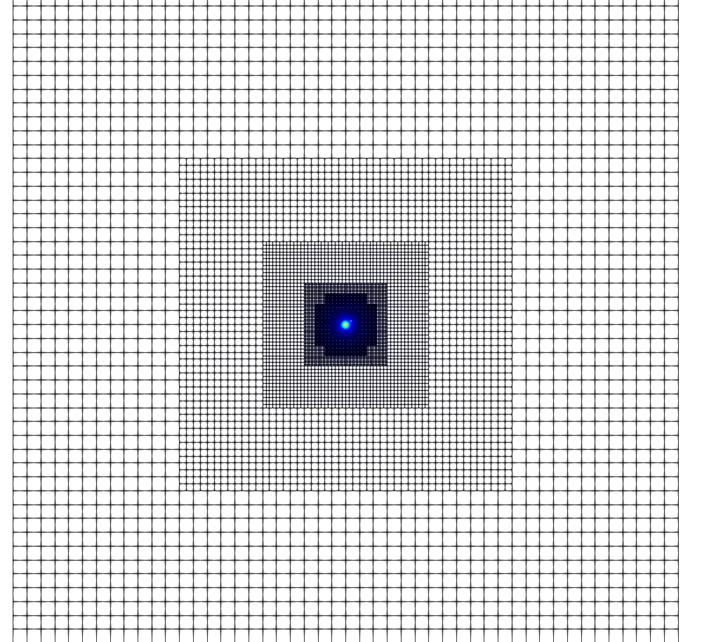
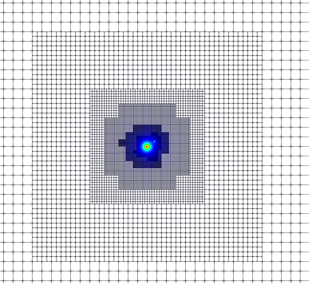
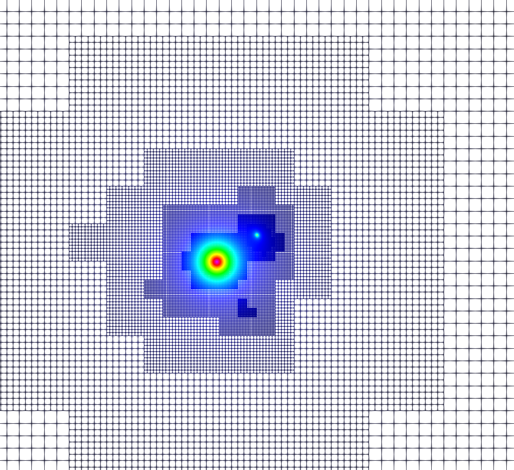
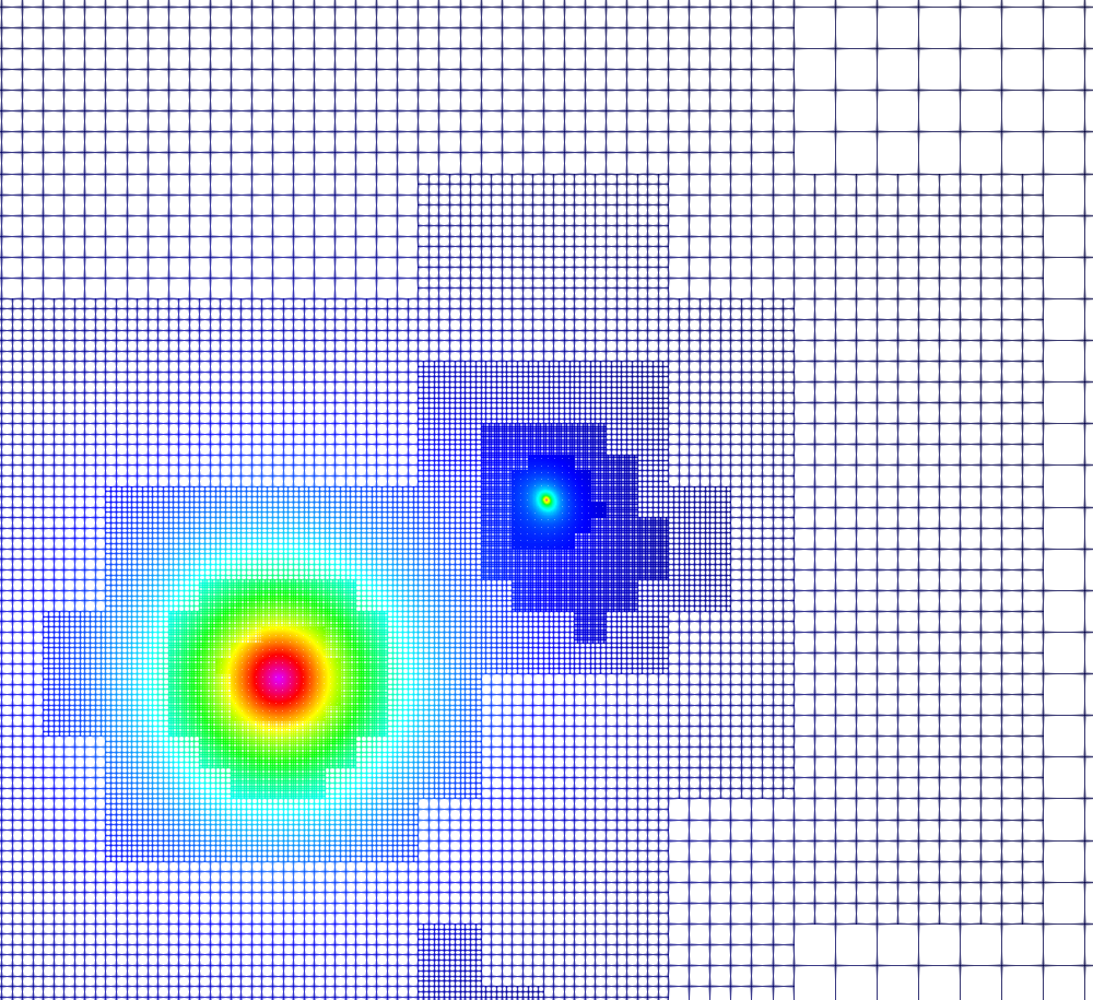
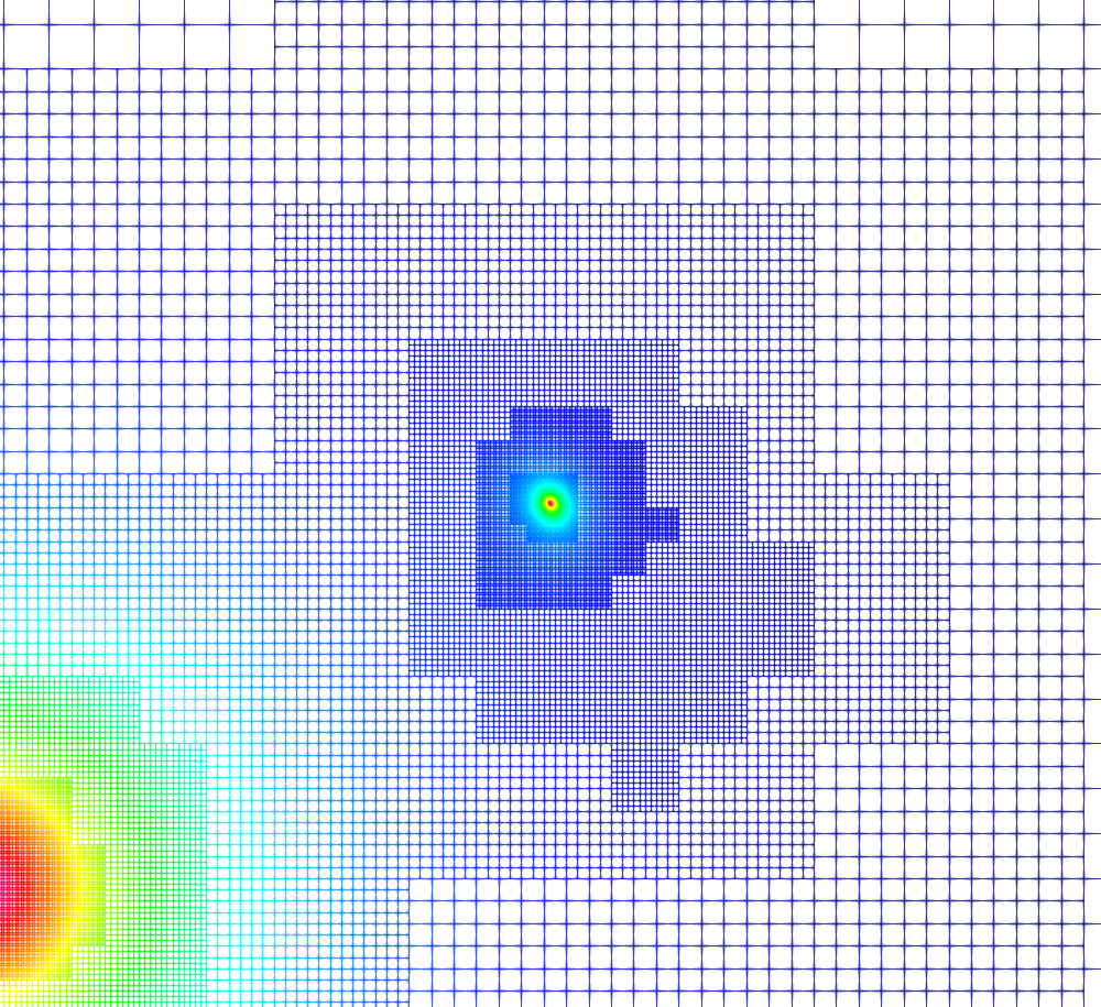
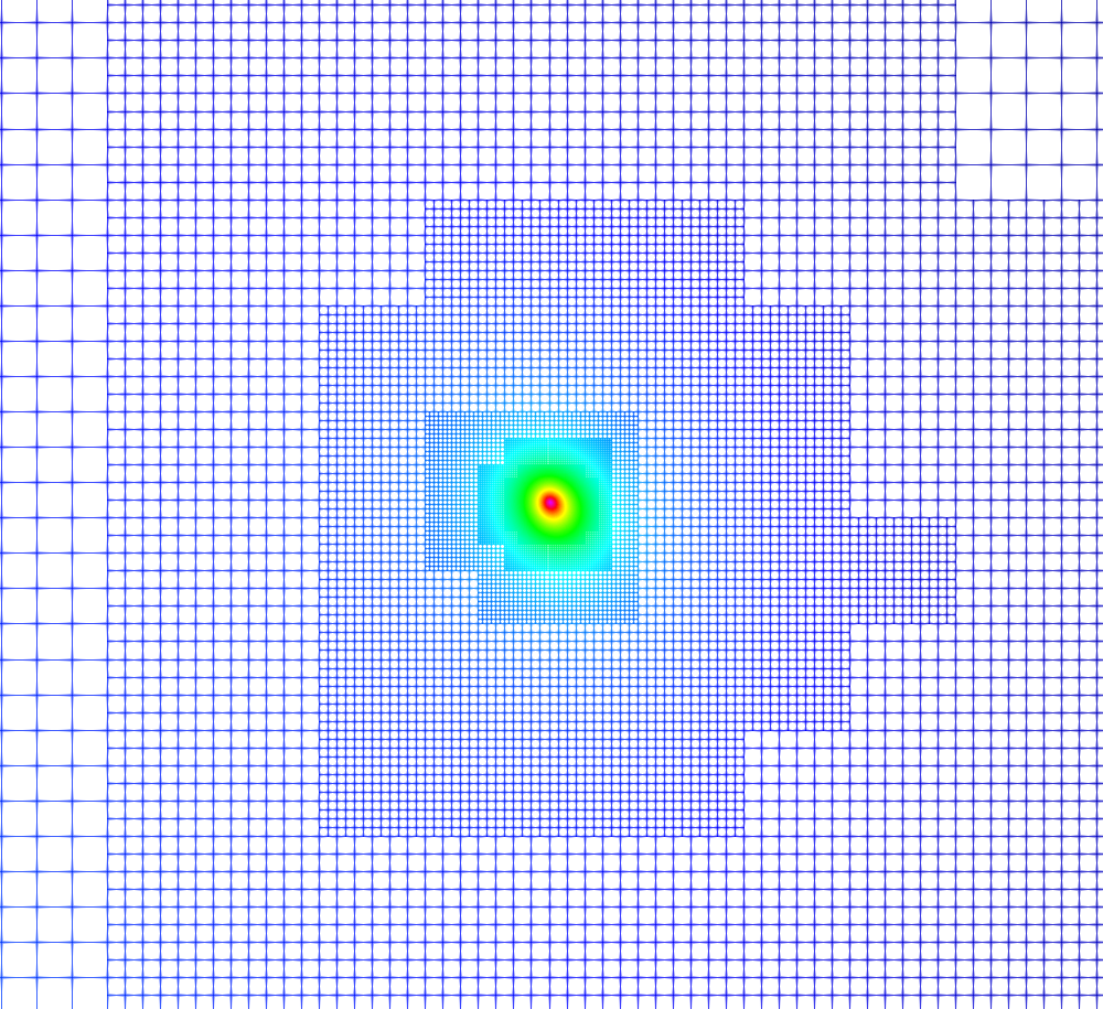
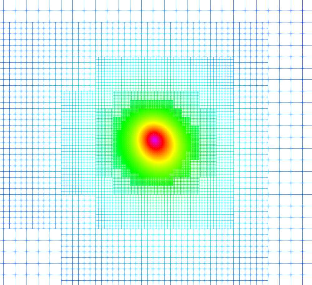
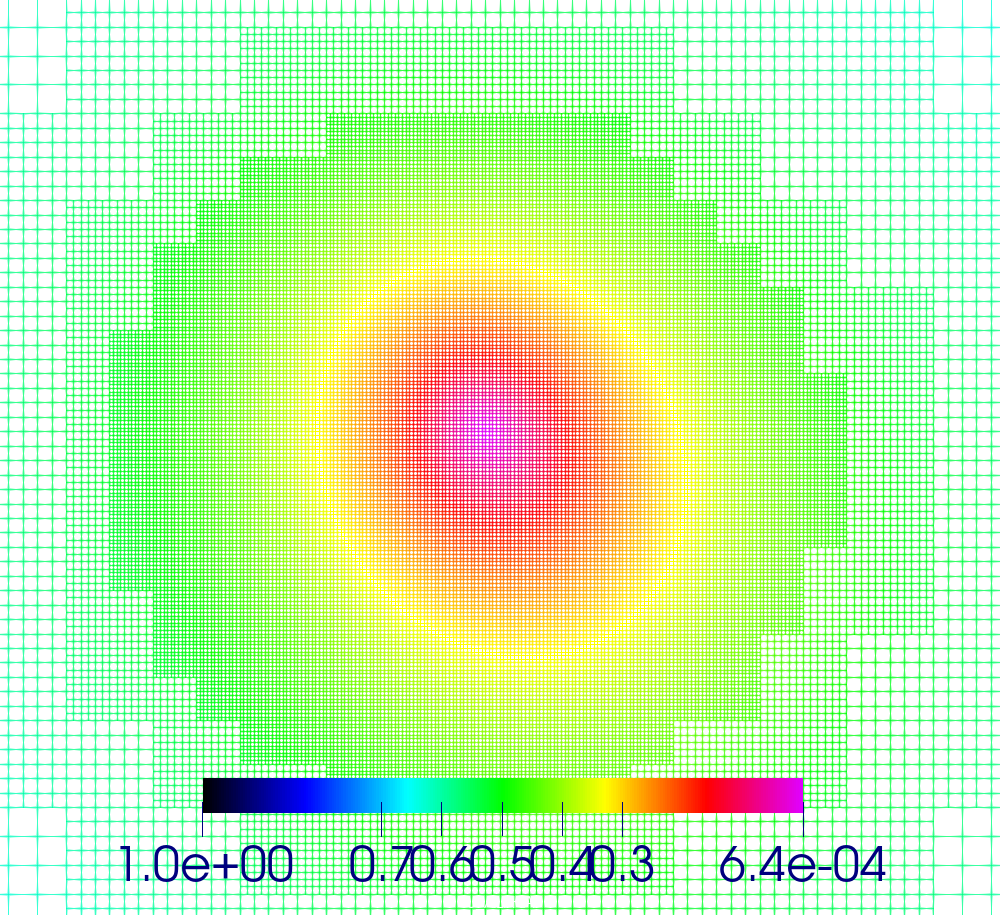
Figure 3: This figure plots the lapse on the computational grid generated for a $q=16$ black hole binary, after the system has evolved for two orbits. The top left frame shows the entire computational domain, and moving to the right each frame successively zooms in towards the smaller of the two black holes. The computational grid is sparse, with refinement concentrated about the black holes, making it very computationally efficient. The 2:1 refinement constraint for constructing the grid, discussed in Sec. II.6.2, is also apparent in the overall grid structure.

An example of the WAMR-constructed grid used to evolve binary black holes is shown in Fig. 3, which shows the grid for a $q=16$ binary before merger. This computational grid is very efficient: the grid is sparse with refined regions that adapt to the small-scale features of the spacetime. The grid does not require refined regions to be rectangular on large scales, significantly saving on computational and memory costs. Moreover, large overlapping regions between refinement levels are not required.

II.5 Refinement Functions

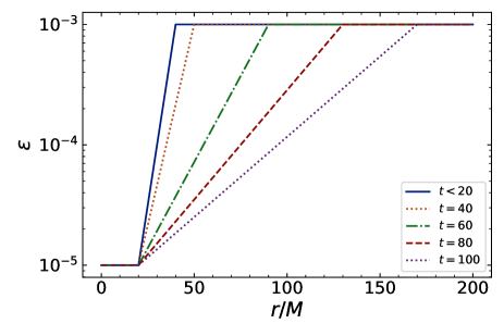
Figure 4: This figure shows the wavelet tolerance, $\epsilon(r)$, for refinement function RF3 at a few representative times. This refinement function is spherically symmetric, centered on the origin of the grid, and is independent of the black hole masses. The minimum wavelet tolerance is used over a relatively large region at the center of the grid. After $t=20M$, the wavelet tolerance decreases in the GW extraction zone, $50<r/M<100$, allowing the initial junk radiation to pass before triggering refinement in this region.

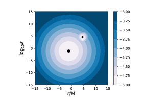
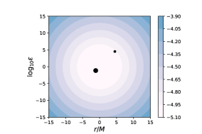
Figure 5: This figure shows the wavelet tolerance, $\epsilon(r)$, using refinement function RF4 for a $q=4$ binary at two times, $t=0$ and $t=40M$. The black dots indicate representative positions and relative coordinate sizes for the two black holes, though not necessarily the physical horizons. This refinement function has the minimum tolerance centered about each black hole. After $t=20M$, the refinement function becomes spherically symmetric and centered at the grid origin, with $\epsilon$ decreasing in the wave extraction region, similar to RF3.

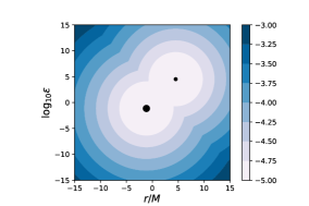
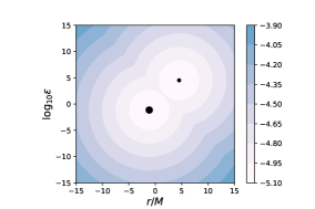
Figure 6: This figure shows the wavelet tolerance, $\epsilon(r)$, using refinement function RF5 for a $q=4$ binary at two times, $t=0$ and $t=40M$. The black dots indicate representative positions and relative sizes for the two black holes, however, not the physical horizons. This refinement function has the minimum tolerance centered about each black hole. After $t=20M$, the refinement function reduces to a functional form similar to RF3, but centered about each black hole, rather than the grid’s origin.

Interpolating wavelets are sensitive to any non-differentiable or non-convergent parts of a solution, triggering immediate refinement. This is important for resolving small-scale features in solutions. However, refinement can be triggered by uninteresting or unphysical features as well. In binary black hole spacetimes, we are primarily interested in resolving the binary at the center of the grid and following radiation out to the extraction region. To achieve computational efficiency, therefore, it is important to control where refinement occurs, focusing on physically interesting features in the solution.

One way to manage refinement in Dendro-GR is to set a maximum allowed level of refinement for the entire grid, $J_{\rm max}$. This limit is enforced globally for all times, and is chosen to allow for an expected minimum grid resolution. It is important to note that the spacetime at the black hole puncture is not smooth, and the WAMR grid will continue refining on this feature until the maximum level of refinement is reached. As we evolve binaries with large mass ratios, we need to prevent over-refinement of the more massive black hole in the binary. We modify the naive use of $J_{\rm max}$ by tracking the black hole locations and imposing a mass dependent constraint on the maximum refinement level about each black hole. We refine a sphere expected to extend beyond the apparent horizon to the local maximum refinement level.

Recall that refinement in WAMR is controlled by the wavelet tolerance $\epsilon$. Usually, $\epsilon$ is taken to be a constant. However, we have found that using a spatially-dependent wavelet tolerance, $\epsilon=\epsilon(r)$, allows us to focus refinement near the center of the grid and to reduce refinement beyond the wave extraction zone. We typically choose minimum and maximum values of $\epsilon$, for the inner and outer regions of the grid, respectively, and let $\log\epsilon$ vary linearly between these limits.

Unfortunately, the situation is further complicated by junk radiation in the initial data and time-dependent gauge effects as the initial data relax onto the grid. This latter effect includes a fast moving gauge wave whose frequency becomes higher with increasing mass ratio, $q$. These features trigger substantial refinement as $q$ increases. Over-refining on this high-frequency radiation is a waste of computational resources. In order to limit over-refinement at early times, we have also found it beneficial to make $\epsilon$ a function of time near the beginning of the run.

For the purposes of this work, we define three refinement functions, labelled RF3, RF4, and RF5. RF3 is time-dependent, spherically symmetric, and linear in $\log\epsilon$, as shown in Fig. 4. This refinement function works quite well for smaller values of $q$, such as $q\lesssim 5$. As $q$ increases, however, this refinement function results in prohibitively expensive runs because of spurious waves originating around the smaller black hole. As a result, we introduce an additional spatial dependence to the refinement functions at early times, RF4 and RF5, to more sharply focus refinement at early times around the individual black holes. Figs. 5–6 show these two refinement functions at $t=0$ and $t=40M$. Beyond $t=40M$, these refinement functions become identical to RF3. Notice that refinement is concentrated in a region around the origin and the binary system, with $\epsilon$ increasing at larger radii. Both are also tuned in time to allow for sufficient resolution of the outgoing radiation in the extraction region, while limiting refinement on the initial burst of spurious radiation.

We note that the definitions of these refinement functions are ad hoc, and tuned to the specific runs reported here through experimentation. When used with sufficient resolution, the refinement functions do not appear to interfere with or change significantly the convergence properties of Dendro-GR, as discussed in Sec. IV below, while significantly improving the computational efficiency of the runs. In future work, we will explore generalizations that could be more widely applicable.

II.6 Octree

II.6.1 Octree partitioning

Octree based adaptive space discretizations (see Fig. 7) are commonly used in computational science applications [59, 60, 61, 62, 63, 47, 55]. Using octrees as the underlying data structure for spatial discretization is advantageous due to its simplicity, intrinsic hierarchical structure and relative ease of use in designing scalable parallel algorithms.

In octree based adaptive multiresolution (AMR) applications, the local number of octants changes rapidly as the grid adapts and attempts to capture the spatially varying solution. This will create load imbalances between partitions that can reduce parallel performance. In order to maintain good load balancing, we need fast and efficient partitioning algorithms which, preferably, scale like $\mathcal{O}(n)$ where $n$ is the number of octants. Doing so will also reduce the overall communication cost between partitions. To this end, we use space filling curves (SFC) [64] with a flexible partitioning scheme [55]. Based on the order with which these curves traverse the octants, we are able to define a partial ordering operator on the octree domain, which, in turn, is used to sort the octree. Once this happens, higher dimensional partitioning reduces to a 1D problem along a curve.

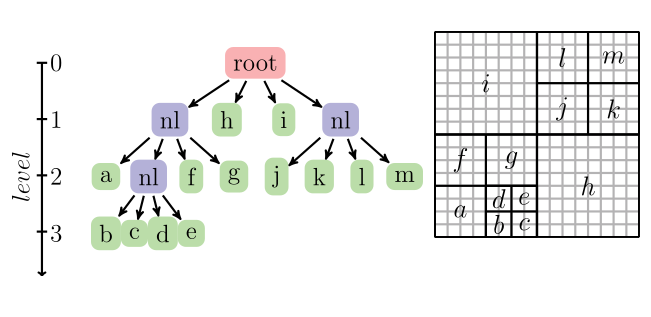
Figure 7: A simple illustration of a 2D quadtree (in 3D, it would be an octree) as a data structure to represent a 2D adaptive grid. Note that we start from the root level, and perform a hierarchical division of each dimension to generate spatially varying resolution on the computational domain. In terms of storage, we only store the leaf nodes of the tree since non-leaf nodes can be computed by performing a top-down or bottom-up traversal of the tree.

Figure 8: This figure shows a $2D$ example of the octant local (center) and octant shared (right) nodal representation (with $d=2$) of the adaptive quadtree shown on the left. Note that the octant local representation has grid points that are local to each octant and contains duplicate grid points in neighboring octants. By removing duplicate and hanging grid points we get the octant shared representation. In this figure, grid points are color coded based on the octant level.

II.6.2 Octree construction and balancing

Octree construction is the process of creating an adaptive octree discretization to capture a function $f:\Omega\rightarrow\mathcal{R}^{n}$ defined on a computational domain $\Omega$. The wavelet expansion of $f$ determines the adaptive structure for the user-specified tolerance function $\epsilon$. Initially, we begin from the root level of the octree and continue refining if the computed wavelet coefficients are greater than $\epsilon$. In our case, with the BSSN equations, the initial grid is generated based on two puncture initial data (§II.2). All processes begin from the root level and continue refinement until at least $p$ octants are produced (where $p$ denotes the number of processes). These $p$ octants are equally partitioned across processes. Further refinement occurs in an element-local fashion. As the number of octants increases with refinement, the octree is periodically re-partitioned to ensure load balancing.

We enforce an additional constraint on the octree during refinement which we refer to as “2:1 grid balancing.” [65] This particular constraint enforces the condition that for a given octant in the octree, all of its geometric neighbors (faces, edges, and vertices) differ, at most, by a single level. Imposing this constraint ensures that the refinement structure varies smoothly through the entire grid. Moreover, we are guaranteed a correct interpolation stencil for points at level $j$ from points at level $j-1$. As a result, this simplifies the subsequent mesh generation process significantly.

II.6.3 Mesh generation

In order to perform numerical computations, the octree requires the notion of neighborhood information. The number of grid points placed in each octant depends on the degree of the finite difference stencil or polynomial interpolant used. For $d^{th}$-order finite differences, $(d+1)^{3}$ points are placed on each octant. We refer to this representation as octant local. The wavelets are calculated via interpolations of the same order. As octants are shared through faces, edges, and vertices, neighboring octants will contain redundant informaton. These are efficiently identified and then removed in order to get the octant shared  respresentation (see Fig. 8). We have two mappings between these two data representations which allow for finite difference stencil computations of arbitrary order.

Figure 9: This figure shows a simplified example of the octree to block decomposition and the unzip operation. The left figure shows the octant shared representation. The block decomposition is shown in the middle. Note that the given octree is decomposed into four regular blocks of different sizes. The right figure shows the decomposed blocks padded with values coming from neighboring octants with interpolated points when needed to give local uniform blocks.

II.6.4 Evaluating the equations

All the field variables are defined in the compact octant shared, or zipped, representation. This zipped representation allows for efficient low overhead inter-process communication. However, to enable finite-difference (FD) computations, it is necessary to decompose the adaptive octree into smaller regular grid patches or blocks. Following this decomposition from the octree to a block, we compute a padding region for which the width depends on the maximum FD stencil radius (see Fig. 9). The unzipped representation denotes the octant local representation together with the padding region constructed from the adaptive octree. This unzipped representation is purely local to each process and discarded after FD stencils are evaluated (see Fig. 9).

III The LazEv Code

The LazEv code [37] was one of the two original codes to implement the moving puncture approach [38, 66]. The current version uses the conformal function $W=\sqrt{\chi}=\exp(-2\phi)$ [67], eighth-order centered finite differencing in space [68] and a fourth-order Runge Kutta time integrator.

The LazEv code uses the EinsteinToolkit [29, 28] / Cactus [69] / Carpet [70] infrastructure. The Carpet mesh refinement driver provides a “moving boxes” style of mesh refinement. In this approach, refined grids of fixed size are arranged about the coordinate centers of both holes. The Carpet code then moves these fine grids about the computational domain by following the trajectories of the two BHs.

The LazEv code implements both the BSSN [71, 72, 73] and CCZ4 [74] evolution systems. For the tests here, we use the BSSN system. For the gauge conditions, we use a modified 1+log lapse and a modified Gamma-driver shift condition [75, 38, 76],

$$(\partial_{t}-\beta^{i}\partial_{i})\alpha = -2\alpha K,$$ (6a)

$$\partial_{t}\beta^{a} = (3/4)\tilde{\Gamma}^{a}-\eta(\vec{x})\beta^{a}\,.$$ (6b)

For the function $\eta$, we choose

$$\eta(\vec{r})=(\eta_{c}-\eta_{o})\exp(-(r/\eta_{s})^{4})+\eta_{o},$$ (7)

where $\eta_{c}=2.0/M$, $\eta_{s}=40.0M$, and $\eta_{o}=0.25/M$. With this choice, $\eta$ is small in the outer zones. The magnitude of $\eta$ limits how large the timestep can be with $dt_{\rm max}\propto 1/\eta$ [77], Because this limit is independent of spatial resolution, it is only significant in the very coarse outer zones where the standard CFL condition would otherwise lead to a large value for $dt_{\rm max}$.

We use AHFinderDirect [78] to locate apparent horizons. We measure the magnitude of the horizon spin using the isolated horizon (IH) algorithm [79]. Note that once we have the horizon spin, we can calculate the horizon mass via the Christodoulou formula

$${m_{H}}=\sqrt{m_{\rm irr}^{2}+S_{H}^{2}/(4m_{\rm irr}^{2})}\,,$$ (8)

where $m_{\rm irr}=\sqrt{A/(16\pi)}$, $A$ is the surface area of the horizon, and $S_{H}$ is the spin angular momentum of the BH (in units of $M^{2}$).

We calculate the radiation scalar $\psi_{4}$ using the Antenna thorn [80, 81]. We then extrapolate the waveform to an infinite observer location using perturbative formulas from [82].

While we use eighth-order centered difference stencils, we use a fifth-order Kreiss-Oliger dissipation stencil and fifth-order spatial prolongation operator (prolongation in time is second-order). We found that a rather large dissipation coefficient of $\epsilon_{\rm dis}=0.4$ gave the best results.

IV Tests

In this section we present some numerical results to demonstrate the overall accuracy and performance of the Dendro-GR framework. We first present results that suggest that the maximum amount of Kreiss-Oliger dissipation should be used when solving BSSN-like formulations of the Einstein equations. Higher amounts of Kreiss-Oliger dissipation increase the rate of convergence observed in our tests. Second, we study binary black hole mergers with mass ratios $1\leq q\leq 16$ using Dendro-GR. We show that these results converge to equivalent solutions obtained using LazEv. Finally, we present results on the numerical performance of Dendro-GR. We discuss some of the refinement challenges in binary black hole spacetimes, and show how different refinement strategies affect the overall computational cost of the solution.

IV.1 Effects of Kreiss-Oliger Dissipation on BBH mergers

Table 2: Some parameters and run-time information for the runs presented in this paper. All runs used wavelet tolerances $\epsilon_{\rm min}=10^{-5}$ and $\epsilon_{\rm max}=10^{-3}$. Runs were performed on Expanse at SDSC.

Run ID	Mass ratio	$J_{\rm max}$	$\Delta x_{\rm min}$	$J_{\rm max}$	$\Delta x_{\rm min}$	RF	SUs	Wall Time
	$q=m_{1}/m_{2}$	(BH2)	(BH2)	(BH1)	(BH1)		(${\rm cpu}\cdot{\rm hrs}$)	(hrs)
q1A	1	15	4.069e-3	15	4.069e-3	2	–	–
q2RF3l	2	15	4.069e-3	14	8.138e-3	3	5 540	43
q2RF3m	2	16	2.034e-3	15	4.069e-3	3	41 170	80
q2RF3l	2	15	4.069e-3	14	8.138e-3	4	5 229	41
q2RF4m	2	16	2.034e-3	15	4.069e-3	4	39 521	77
q4	4	16	2.034e-3	14	8.138e-3	3	22 717	89
q8RF3	8	18	5.086e-4	14	8.138e-3	3	485 810	483
q8RF4	8	18	5.086e-4	14	8.138e-3	4	101 915	318
q8RF5	8	18	5.086e-4	14	8.138e-3	5	64 477	263
q16RF4	16	19	2.543e-4	14	8.138e-3	4	799 590	1 149
q16RF5	16	19	2.543e-4	14	8.138e-3	5	–	–

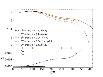
Figure 10: This figure shows the effect of Kreiss-Oliger dissipation on the $q=1$ binary BH merger using the LazEv code. Shown are results of the binary separation versus time using both different finite difference orders and different dissipation amplitudes ($\sigma$). The top frame plots the coordinate separation ($r$) between the BHs as a function of coordinate time for runs with large ($\sigma=0.4$) and small ($\sigma=0.04$) Kreiss-Oliger dissipation, different finite difference orders ($4,6,8$) and at two resolutions. The three high dissipation cases computed with different FD orders are indistinguishable on this plot (solid and dashed dot curves). In contrast, the small dissipation cases are significantly different, while clear convergence is seen. The lower panel plots the difference between the 4th and 6th-order results ($r_{46}=r_{\rm 4th}-r_{\rm 6th}$) and the 6th and 8th-order ($r_{68}=r_{\rm 6th}-r_{\rm 8th}$) results for $\sigma=0.4$. Note that even though the corresponding three curves in the top panel are indistinguishable, clear convergence with increasing order is seen in the lower panel. Note that $h$ indicates the coarsest resolution of the AMR grid and $h_{0}=3.3M$.

Kreiss-Oliger dissipation is widely used in numerical relativity. This dissipation is explicitly added to the numerical scheme to eliminate high-frequency noise that can arise in the evolution, especially near the puncture, where spacetime variables are non-differentiable and at refinement boundaries. A common expectation is that one should minimize the amount of explicit dissipation provided that high-frequency noise is well controlled. However, when performing the initial comparisons of results from binary black hole mergers with Dendro-GR and LazEv, we found the opposite to be true.

In our tests, the fifth-order Kreiss-Oliger dissipation operator in Eq. 5 is added to the RHS of the semi-discrete equations with the parameter $\sigma$, $0\leq\sigma<1$. We performed multiple binary black hole mergers for $q=1$ with different values of $\sigma$ using both LazEv and Dendro-GR. Results from LazEv  are shown in Fig. 10, which plots the coordinate separation between the two black holes. This figure shows that the runs with small dissipation, $\sigma=0.04$, differ from those with large dissipation, $\sigma=0.4$. Further, the solution with small dissipation converges towards those with large dissipation with increasing resolution. Curiously, for the runs with large dissipation, the order of the spatial finite derivatives, fourth order vs sixth, and the order of the Kreiss-Oliger dissipation operator, fifth vs ninth, was not as important as the amount of dissipation, i.e., the value of $\sigma$. Similar results were obtained with Dendro-GR.

This result is counter-intuitive, and we are not aware of a similar discussion in the literature. The numerical noise in the $\sigma=0.04$ runs was well-controlled, and visual inspection of the solutions did not indicate potential problems. However, when solving the BSSN equations for black hole spacetimes, better solutions at lower resolutions are obtained using larger amounts of explicit numerical dissipation.

IV.2 Convergence tests for Dendro-GR and LazEv

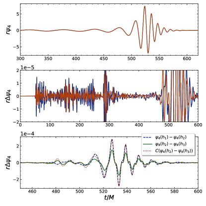
Figure 11: Convergence test of a $q=1$, non-spinning binary using LazEv. The top panel shows the low and high resolution waveforms. The middle panel shows the differences in the waveforms between the low and medium resolutions (in blue) and the medium and high resolutions (in red). Because the waveforms are of comparable size, initially there is small, but non-convergent noise (at these resolutions). The bottom panel shows the differences rescaled, assuming $3.5$ order convergence, at the peak of the waveform. At the peak, the stochastic AMR noise is smaller than the truncation error.

Convergence is an important test not only of the computational code, but it is also the only way to establish an estimate of the overall error in the waveform. To test the convergence of both codes, we evolved initial data for an equal mass ($q=1$), non-spinning binary. The initial data parameters are shown in Table 1. For the $q=1$ binary, we ran the LazEv code at three resolutions, $\Delta x=h_{0}$, $h_{0}/1.2$ and $h_{0}/1.44$ with $h_{0}=3.3M$, on the coarsest grid with nine levels of refinement. As shown in the center panel of Fig. 11, the waveform is not initially convergent, as relatively small stochastic errors owing to reflections of high-frequency spurious radiation off the refinement boundaries dominate the error. As these high-frequency waves dissipate and the physical signal gets larger, convergence of the error becomes clear. The bottom panel shows that the waveform is convergent for the late inspiral at order 3.5. Note that Fig. 10 also shows convergence of the radial separation for the $q=1$ case. The $q=2$ binaries were run with base resolutions of $h_{0}/1.2$ and $h_{0}/1.4$, but added an additional level of refinement around the smaller BH. Similar convergence results were obtained for $q=2$. Finally, for $q=4$, we ran with a base resolution of $h_{0}/1.2$ and added two additional refinement levels (compared to $q=1$) about the smaller black hole.

Dendro-GR uses an unstructured grid, and convergence is both more difficult to define and more challenging to demonstrate. Convergence depends both on the spatial resolution, $\Delta x$, as well as the wavelet tolerance, $\epsilon$. Fig. 12 shows the convergence of Dendro-GR solutions (for $\psi_{4}$) at two resolutions, labeled low (runs q2RF3l and q2RF4l) and medium (q2RF3m and q2RF4m) , for $q=2$ binaries. The highest resolution LazEv $\psi_{4}$ is also plotted for comparison. With respect to changing $\Delta x$, the low and medium resolution runs converge to the LazEv solution.

As mentioned above, we choose the wavelet tolerance $\epsilon$ to be a function of both time and space in Dendro-GR. Thus choosing different refinement functions can also potentially affect the solution. Fig. 12 also shows this effect by plotting results from two different wavelet refinement functions, RF3 and RF4, for each resolution. In this case, the effect of changing the refinement function had a relatively small effect on the solution and the overall runtime, see Table 2.

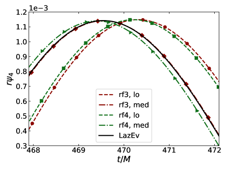
Figure 12: This figure shows the convergence of Dendro-GR solutions with decreasing $\Delta x$. For $q=2$, GW solutions were computed at two resolutions with two refinement functions with fixed $\epsilon_{\rm min}$. The low resolution runs are plotted with dashed lines, with some representative points indicated with circles and squares. The higher resolutions runs are plotted with dashed dot lines, and representative points are indicated with triangles and diamonds. The RF3 solutions are in red and the RF4 in green. Both RF3 and RF4 solutions converge to the LazEv solution (solid black line) as the maximum refinement level is increased. The convergence is largely unaffected by the choice of refinement function.

Fig. 13 illustrates the effect of only varying $\epsilon$ on the solution. This figure compares the Dendro-GR waveforms for three values of $\epsilon_{\rm min}=\{10^{-3},10^{-5},10^{-6}\}$ with the highest resolution LazEv waveform, by plotting the difference. Clearly the differences decrease with decreasing $\epsilon$, as smaller values for $\epsilon$ triggers larger refined regions in the octree. While this is a form of convergence with respect to wavelet tolerance, the maximum refinement level, $J_{\rm max}$, and the minimum resolution, $\Delta x_{\rm min}$, are fixed, so this is not convergence in the Richardson sense of the term.

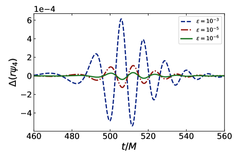
Figure 13: This figure shows convergence with respect to $\epsilon$ given a fixed maximum refinement level. The plot shows the difference between the extracted GWs using the LazEv  and Dendro-GR codes for the real part of the $\psi_{4}$ scalar with decreasing $\epsilon$. The Dendro-GR  solutions with decreasing $\epsilon$ converge to the LazEv  waveforms. Refinement function RF3 was used here.

IV.3 Dendro-GR binaries with different mass ratios

Table 2 gives some refinement and performance information for the Dendro-GR runs reported in this paper. The refinement information includes the maximum allowed refinement level, $J_{\rm max}$, the minimum resolution used in the run, $\Delta_{\rm min}$, and the refinement function. The performance information provides an estimate for the total number of SUs, defined as the number of CPU$\cdot$hours to complete the run. This number is approximated, because Dendro-GR dynamically changes the number of active threads during a run. Finally, the table includes the total wall-clock time used to complete the run. While this information is valuable in providing a general view of Dendro-GR’s performance, we caution that detailed conclusions cannot be drawn. First, the runs in this table were run over a long time period. During this time code changes were made, and parameters were adjusted as we gained experience with the code. These changes impacted the computational costs of the runs. Secondly, wallclock times depend on the number of cores used for each job, the final integration time, the workload per core, etc. For comparison, the LazEv $q=1$ medium resolution run used 27472 SUs, while the high resolution run used 71651 SUs. The LazEv $q=2$ medium resolution run used 100766 SUs, while the high resolution run used 228065 SUs. Finally, the LazEv $q=4$ medium resolution used 169799 SUs, while the LazEv $q=4$ high resolution used 474683 SUs. All the LazEv  runs were performed on the same Intel Skylake cluster. Note that the LazEv  runs were performed at relatively high resolution to ensure that the error in the LazEv simulations is small compared to the Dendro-GR simulations. These high resolution runs are required because we will use the LazEv  simulations to calibrate the accuracy of the Dendro-GR simulations.

Figs. 14–15 show gravitational waveforms computed for non-spinning binaries with mass ratios up to $q=16$. Parameters for the initial data are shown in Table 2, which also gives resolution and refinement function data, as well as the computational cost and time to solution. As noted in Sec. II.2, the initial data for $q\geq 2$ are constructed from a single family of initial data [49], while data for $q=1$ are constructed from ad hoc parameters. For $q=1,2$ and $4$, the figures also show waveforms computed with LazEv. Due to the relativity long walltime required, we chose not to complete the correspondingly high-resolution simulations for $q=4$ simulations. Thus the difference between the Dendro-GR and LazEv waveforms for $q=4$ may only indicate that the LazEv simulation was underresolved. Importantly, due to its scaling, the Dendro simulations were obtained more quickly. The binaries with $q=8$ and $q=16$ were performed only with Dendro-GR. These figures show that Dendro-GR produces gravitational waveforms very similar to LazEv. The mismatch for these different waveforms are calculated below, in Sec. IV.4. Unfortunately, it is difficult to draw conclusions the accuracy of Dendro-GR across different values of $q$, because these runs were performed over a long period of time with changing refinement strategies and a changing code base. Many of the code changes and new approaches were motivated, in fact, in the process of running these cases. We were not able to go back and rerun all cases with the same version of the code and consistent refinement criteria.

As discussed in Sec. II.5, a gauge wave propogates across the computational domain at early times, as the coordinates transition from the Bowen-York gauge conditions, used to calculate the initial data [48], to the puncture gauge conditions used in the evolution. The wavelength of the gauge wave is related to the black hole size, and thus the frequency of this unphysical wave increases with mass ratio, $q$. The high frequency wave triggered excessive refinement at the beginning of the higher mass ratio runs, particularly for $q\geq 8$, prompting our experimentation with different wavelet refinement functions. We ran simulations of the $q=8$ binary with three different refinement functions, and plot the resulting waveforms in Fig. 15. RF3 uses $\epsilon_{\rm min}$ over a larger volume of the grid, while RF4 and RF5 allow for a larger wavelet tolerance over a larger region of the grid. Consequently, RF3 likely gives a more precise solution but at a greater computational cost as it may tend to over-refinement. While RF4 and RF5 are more computationally efficient, differences in the waveforms become noticable. For $q=16$, RF3 was too expensive, and this run was only done with RF4 and RF5. The RF5 run was not completed, as the differences in results for RF3 and RF5 for $q=8$ were large. Interestingly, the differences in RF3 and RF4 occur only at the initial time. After $t=40M$, both refinement functions are identical. The phase differences seen in the figure seem to arise solely from small variations in the refinement at early times.

The number of computational cores used in the $q=8$ and $q=16$ runs are plotted in Figs. 16 and 17, respectively. Dendro-GR regularly repartitions the computational workload across the available cores. To balance the communication cost between cores, it will use fewer cores than the total number available if the workload per core drops below some threshold. In these runs, over-refinement on the high frequency gauge wave and junk radiation remains a problem, and causes the large increase in demand for computational resources at the beginning of the run. As this radiation moves beyond gravitational wave extraction region, the grid is coarsened and the runs become much more efficient.

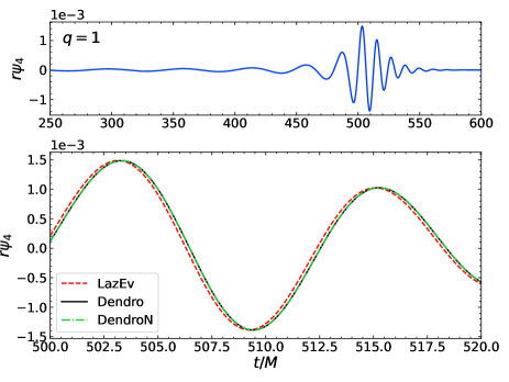
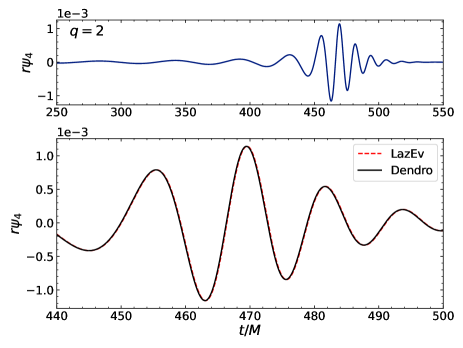
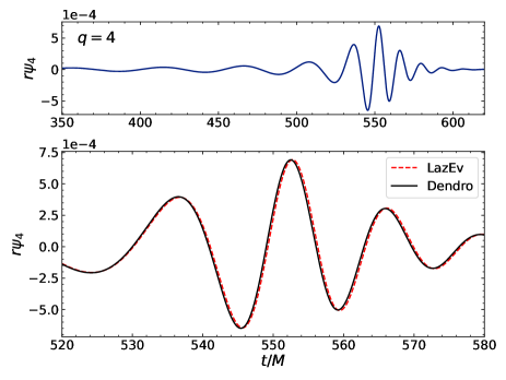
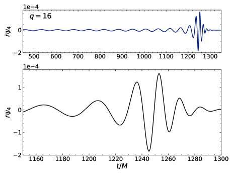
Figure 14: Plots comparing the waveform for the $q=1,2,4,16$ cases. LazEv and Dendro-GR waveforms are given for all except $q=16$, where only Dendro-GR results were produced. This figure plots the real part of $\psi_{4}$ for the highest resolution Dendro-GR and LazEv (where available) runs.

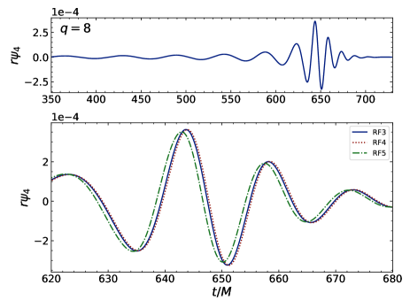
Figure 15: This figure shows the real part of $\psi_{4}$ for a $q=8$ black hole binary, computed with Dendro-GR using three different refinement functions with the same minimum spatial resolution. RF3 has the smallest error tolerance at the center of the grid, but is very computationally expensive. The RF4 solution is quite similar to RF3, but at roughly one fifth of the computational cost (see Table 2). The RF5 solution is the least expensive to compute, but for the parameters used here, the phase error is significant.

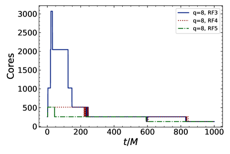
Figure 16: This figure shows the effect of different refinement functions on the computational cost of evolving a $q=8$ black hole binary with Dendro-GR by plotting the number of computational cores used during the simulation as a function of the computational time. The three refinement functions, RF3, RF4, and RF5, differ only for $t\leq 40~{}M$. Thus, the differences arise primarily in how the initial junk radiation and gauge waves are resolved. As shown in Fig. 15, the gravitational wave results from RF3 and RF4 are similar, although the maximum workload for RF4 was about 6 times smaller than the maximum workload for RF3. The results for RF5, while the most efficient run, show larger differences from the other two cases.

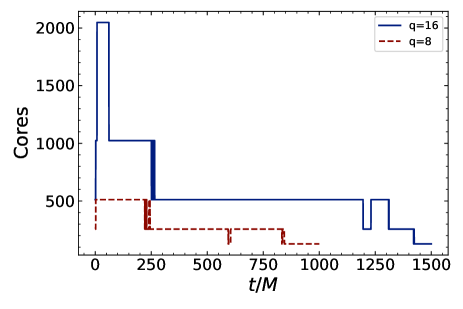
Figure 17: This figure shows the number of computational cores used in $q=8$ and $q=16$ binary black holes merger simulations with RF4.

IV.4 Overlaps

When using numerical waveforms for gravitational wave data analysis, numerical convergence provides an important estimation of the error in the numerical solution. Ideally, the convergence error, determined by comparing the solutions computed at two different resolutions, is smaller than the other errors in the analysis. However, convergence testing overlooks the frequency response of a real-world detector. The overlap provides a way to compare two waveforms as measured in a detector with a given frequency response. In addition, the overlap helps us to determine the computational resources required to simulate a particular configuration. This allows us to determine how similar two waveforms, computed at different resolutions or with different codes, are to one another.

For this analysis, we will measure the consistency of two waveforms using the CreateCompatibleComplexOverlap function in LaLSimUtils (which is freely available) [83, 84]. This function automatically optimizes over both time translations and phase shifts. Because of this, the mode-by-mode mismatch allows for the phase shifts of different modes to be inconsistent. That is, one expects each $m$-mode to be shifted by $m\phi$.

Internally, this function uses the inner product

$$\left\langle h_{1}|h_{2}\right\rangle=2\,\int_{-\infty}^{\infty}\frac{h_{1}^{*}(f)h_{2}(f)}{S_{n}(f)}\mathrm{d}f,$$ (9)

where $h(f)$ is the Fourier transform of the complex waveform $h(t)$ and we use the Advanced-LIGO design sensitivity Zero-Detuned-HighP noise curve [85] with $f_{\text{min}}=20$ Hz and $f_{\text{max}}=2000$ Hz. This inner product is then further maximized over time and phase shifts as described in [86]

$$\left\langle h_{1}|h_{2}\right\rangle=\max_{t_{0},\phi_{0}}\left[\,2\,\left|\int_{-\infty}^{\infty}\frac{h_{1}^{*}(f)h_{2}(f)}{S_{n}(f)}\mathrm{d}f\right|\,\right].$$ (10)

The overlap of two waveforms is then given by

$$\mathcal{O}=\frac{\left\langle h_{1}|h_{2}\right\rangle}{\sqrt{\left\langle h_{1}|h_{1}\right\rangle\left\langle h_{2}|h_{2}\right\rangle}}$$ (11)

and the mismatch is given by

$$\mathcal{M}=1-\mathcal{O}.$$ (12)

Because Eq. (9) directly involves the detector’s noise sensitivity curve, $S_{n}(f)$, the mismatch is a function of the actual frequency waveform and is not invariant under a change in the total mass of the system. Depending on the total mass, only a portion of the waveform may be in the detector’s sensitivity region. As an example, for systems with small total mass, LIGO is most sensitive to the low-frequency portion of the signal at early times. For systems with a large total mass, however, LIGO is most sensitive to the high-frequency merger and early ringdown portion of the waveforms.

We use the mismatch, $\cal M$, to compare the Dendro-GR and LazEv  waveforms. A mismatch of ${\cal M}<0.005$ was determined in Ref. [87] to be minimally acceptable for advanced LIGO analysis. Ideally, a mismatch ${\cal M}\ll 0.005$ is desired. However, this limit of $<0.005$ is for the net mismatch in the observed waveforms (i.e., after summing all modes). Setting the mismatch tolerance to $<0.005$ for all subdominant modes is therefore more restrictive than required. Here, we want to use the mismatch between the LazEv and Dendro-GR simulations to measure the truncation error in the Dendro-GR simulations. This is only true if the error in the LazEv simulations is much smaller than the Dendro-GR simulations. To an attempt to guarantee this, we require that the corresponding LazEv-to-LazEv mismatches (between the medium and high resolutions) are much smaller than the corresponding LazEv-to-Dendro-GR mismatches (we note that a small LazEv-to-LazEv mismatch may not account for all possible global errors). When this is not the case, the mismatch between the two codes is not a measure of the error of the Dendro-GR simulations. Figs. 18 - 20 show the overlaps for different modes of $\psi_{4}$ computed with Dendro-GR  and LazEv, for the $q=1$, $q=2$, and $q=4$ binaries, respectively. In particular, we use the high-resolution LazEv solutions as the base solutions for comparison with the Dendro-GR and medium-resolution LazEv waveforms. The figure shows the modes in order of decreasing amplitude. The $q=1$ subdominant Dendro $(2,0)$ mode shows a significant mismatch with the corresponding LazEv mode. All modes with amplitude larger than the $(2,0)$ mode show much smaller mismatches between Dendro and LazEv. The $q=2$ and $q=4$ comparisons show similar behavior (here, more modes are non-trivial, and the $(2,0)$ mode is subdominant to all modes shown).

Fig. 21 shows the overlaps in the $(\ell,m)=(2,-2)$ mode of $\psi_{4}$ for Dendro-GR waveforms computed with different refinement criteria. These overlaps compare solutions computed with different refinement functions, RF3 and RF4, with a refinement tolerance $\epsilon=10^{-5}$. The figure also shows the overlap for a solution computed with RF3 and the refinement tolerance set to $\epsilon=10^{-6}$. The main result from this figure is that higher resolution (more restrictive error tolerance) leads to a better agreement between LazEv and Dendro. Finally, the overlap of the medium-resolution LazEv solution is shown. Consistent with the earlier convergence results, the Dendro-GR runs match the high-resolution LazEv solution well, and the RF3 solution is slightly closer. Finally, Fig. 22 shows the overlap of the Dendro-GR solutions for the $q=8$ binary computed with the RF3 and RF4 refinement functions.

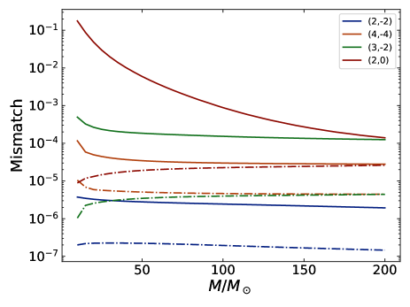
Figure 18: This figure shows the overlaps in gravitational waveforms for various modes of the Dendro-GR and LazEv solutions for a $q=1$ binary. The dot-dashed lines show the overlaps of the LazEv  medium resolution waveforms against the LazEv high-resolution waveforms. The solid lines show the overlaps of the Dendro-GR waveforms against the LazEv high-resolution waveforms. The modes are presented in order of decreasing amplitude. The $(2,0)$ mode, which fails our accuracy goal of ${\cal M}<0.005$ is subdominant to all the other modes.

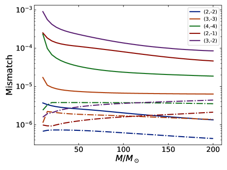
Figure 19: This figure shows the overlaps in gravitational waveforms for various modes of the Dendro-GR and LazEv solutions for a $q=2$ binary. The dot-dashed lines show the overlaps of the LazEv  medium resolution waveforms against the LazEv high-resolution waveforms. The solid lines show the overlaps of the Dendro-GR waveforms against the LazEv high-resolution waveforms. The modes are presented in order of decreasing amplitude (i.e., (3,-3) is subdominant to (2,-2), (4,-4) to (3,3), etc.).

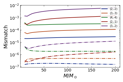
Figure 20: This figure shows the overlaps in gravitational waveforms for various modes of the Dendro-GR and LazEv solutions for a $q=4$ binary. The dot-dashed lines show the overlaps of the LazEv  medium resolution waveforms against the LazEv high-resolution waveforms. The solid lines show the overlaps of the Dendro-GR waveforms against the LazEv high-resolution waveforms. The modes are presented in order of decreasing amplitude (i.e., (3,-3) is subdominant to (2,-2), (4,-4) to (3,3), etc.).

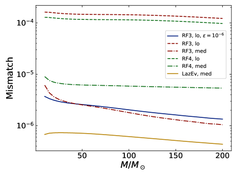
Figure 21: This figure shows the overlaps in the $(\ell,m)=(2,-2)$ mode of $\psi_{4}$ computed with various Dendro-GR refinement criteria against the high-resolution LazEv solution for a $q=2$ binary. The blue line is computed with $\epsilon=10^{-6},$ and all other cases use $\epsilon=10^{-5}$. As expected, the waveforms computed with the more expensive RF3 refinement function (red) have better overlaps to LazEv than those computed with RF4 (green). Finally, the tan solid line shows the overlap of the LazEv  medium and high resolution waveforms.

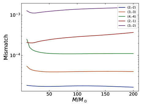
Figure 22: This figure shows the overlaps in the Dendro-GR  $q=8$ gravitational waveforms computed with the RF3 and RF4 refinement functions. The waveforms are presented in order of decreasing amplitude. As expected, the dominant modes have smaller mismatches than the subdominant modes.

V Discussion

This paper presents binary black hole evolutions performed with Dendro-GR for different mass ratios up to $q=16$. We present validation tests in comparison with results from LazEv, and we give performance information for these runs.

While the focus of this paper is on evolving binary black holes with Dendro-GR, the first result that we presented has general applicability in the numerical relativity community. We found that in binary black hole evolutions with the BSSN formalism, the rate of convergence is increased when a large amount of Kreiss-Oliger dissipation is added to the solution. In our tests, runs with a dissipation parameter of $\sigma=0.4$ had a better rate of convergence than runs with $\sigma=0.04$, where $\sigma$ is bounded by $\sigma<1$ for numerical stability.

While the performance and scaling of Dendro-GR is very good, we are currently working on additional improvements. In particular, we are improving the unzip process, in which an octant of the tree in locally expanded to a uniform Cartesian grid, to reduce the communication overhead. As shown in this paper, we have started exploring different ways to control the refinement algorithm, especially during the initial times of an evolution. We want to improve the computational performance of Dendro-GR, while not sacrificing the accuracy of the solutions. While we have had some initial success, much more work remains to be done. We continue working on a more general method to monitor errors in the evolution of black hole spacetimes. Finally, in an independent project, we are developing a version of Dendro-GR that runs primarily on GPUs.

The version of Dendro-GR used to produce the results in this paper is distributed subject to the MIT license at https://github.com/paralab/Dendro-GR.