Test-beds and applications for apparent horizon finders in numerical relativity

Abstract

We present a series of test beds for numerical codes designed to find apparent horizons. We consider three apparent horizon finders that use different numerical methods: one of them in axisymmetry, and two fully three-dimensional. We concentrate first on a toy model that has a simple horizon structure, and then go on to study single and multiple black hole data sets. We use our finders to look for apparent horizons in Brill wave initial data where we discover that some results published previously are not correct. For pure wave and multiple black hole spacetimes, we apply our finders to survey parameter space, mapping out properties of interesting data sets for future evolutions.

]

I Introduction

The ability to find black holes, if they exist, in numerically generated spacetimes is an important and difficult problem in numerical relativity. Many algorithms have been developed over the years, but few have been tested extensively on numerically computed spacetimes, and even fewer have been applied to full three-dimensional (3D) spacetime constructions in Cartesian coordinates, which is the most common choice for 3D numerical relativity. As we review below, black holes may exist through topological construction or high concentrations of mass-energy in the initial data, may form through collapse of matter or pure gravitational waves, and may move through the spacetime. The dynamical and numerical properties of black holes in numerical relativity make this a very challenging problem, yet one that must be solved if we are to understand the physics of such simulations, or even if we are to evolve the systems for long periods of time. In this paper we investigate and compare the properties of several algorithms developed to find black holes on an extensive series of analytic and numerically generated spacetimes. We show that due to the sensitive nature of this problem, some previously published results on the existence of apparent horizons in numerically generated spacetimes are incorrect. We also show examples where finders could pass certain test-beds, but failed on more complex cases, revealing coding errors, and also how in some cases existing algorithms had to be modified in order to locate difficult-to-find horizons. Finally, we use these newly developed horizon finders to map out the parameter space of a series of black hole and gravitational wave data sets not yet studied in preparation for future numerical evolutions.

Black holes are defined by the existence of an event horizon (EH), the surface of no return from which nothing, not even light, can escape. The event horizon is the boundary that separates those null geodesics that reach infinity from those that do not. The global character of such a definition implies that the position of an EH can only be found if the whole history of the spacetime is known. For numerical simulations of black hole spacetimes in particular, this implies that in order to locate an EH one needs to evolve sufficiently far into the future, up to a time where the spacetime has basically settled down to a stationary solution. Recently, methods have been developed to locate an analyze event horizons in numerically generated spacetimes, with a number of interesting results obtained [1, 2, 3, 4, 5, 6].

In contrast, an apparent horizon (AH) is defined locally as the outer-most marginally trapped surface [7], i.e. a surface such that the expansion of out-going null geodesics is zero. An AH can therefore be defined on a given spatial hypersurface. A well known result [7] guarantees that if cosmic censorship holds and an AH is found, then an EH must exist somewhere outside of it and hence a black hole has formed.

Being able to find an AH has become a very important issue in the numerical studies of black hole spacetimes. An important reason for this is the development of the so-called apparent horizon boundary condition (AHBC), which excises singularity containing regions interior to the AH in order to extend the evolution. The basic idea behind this is the fact that since the interior of a black hole is causally disconnected from the rest of the spacetime, one can in principle safely ignore it in a numerical evolution, thus avoiding the problem of having to deal with the singularity through the use of a pathological time slicing. Several schemes are being currently implemented to deal with such AHBC [8, 9, 10]. The AH can also be used to determine important information about the spacetime itself; its topology (e.g., multiple disconnected 2–spheres) and its geometry (e.g., its area and local curvature) provide important details of the dynamics of the black holes present in the spacetime [1, 11, 12, 13]. Here we will not deal with such issues, but rather with the problem of finding the AH in a reliable way in the first place.

Many different methods for locating AHs have been developed in the past years, both for axisymmetric (2D) and fully 3D spacetimes [14, 15, 16, 17, 18, 19, 20, 21, 22, 23, 24, 25]. Since even in exact black hole solutions the position of an AH usually has to be determined numerically (with the exception of trivial cases like a Schwarzschild or Kerr black hole), we have found it very useful to develop several independent apparent horizon finders (AHF), using different algorithms and even written by different people. Comparing the results of these AHFs has allowed us both to make careful studies of the horizon structures of a series of spacetimes, and also to compare the performance of the different algorithms. Our tests include simple toy spacetimes, single and multiple black hole spacetimes, and pure gravitational wave spacetimes. With respect to the latter, we have in fact been able to show that some previously published results are not correct.

When comparing the different AHFs we have concentrated both on the reliability with which they can locate an AH and also on the speed at which they can do this. While speed is not such a fundamental consideration when looking for AHs on one given spatial geometry (it only needs to be done once, so one can afford to wait), it becomes of crucial importance when trying to locate them on an evolving spacetime, as will be required in any successful implementation of an AHBC. An AHF that takes much longer than an evolution step to locate an AH can not be used very often without having a disastrous impact on the performance of an evolution code.

A final word on our terminology: Since in this paper we will not deal with the problem of finding event horizons, from now on we will use the term ‘horizon’ to mean always a marginally trapped surface. As we will see in the examples below, there can often be more than one such surface. The AH will be by definition the outermost and we will refer to those marginally trapped surfaces that lie inside it as ‘inner horizons’.

II Finding Apparent Horizons

A Basic Equations

An AH is defined as the outer-most marginally trapped surface [7], that is, a surface where the expansion of out-going null geodesics vanishes. In order to find a mathematical expression for this definition, let us start by considering a smooth spacelike hypersurface $\Sigma$ embedded in a spacetime $(M,g_{\mu\nu})$ (in the following we will use the Greek alphabet to denote spacetime indices on $M$, and the Latin alphabet to denote spatial indices on $\Sigma$). Let $\gamma_{ij}$ and $K_{ij}$ be the induced 3-metric and extrinsic curvature of $\Sigma$, respectively. Let now $S$ be a closed smooth two-dimensional surface embedded in $\Sigma$, with unit outward pointing normal vector $s^{\mu}$. The expansion $H$ of a congruence of null rays moving in the outward normal direction to $S$ can then be shown to be [26]

$$H=\nabla_{i}s^{i}+K_{ij}s^{i}s^{j}-{\rm tr}K,$$ (1)

where $\nabla_{i}$ is the covariant derivative associated with the 3-metric $\gamma_{ij}$. An AH is then the outer-most surface such that $H=0$ is everywhere on the surface (and the surface is smooth).

Let us now rewrite Eq. (1) by assuming that our surface has been parameterized as a level set

$$F(x^{i})=0.$$ (2)

It is now straightforward to rewrite H in terms of the function $F$ and its derivatives. First, we write the unit normal vector $s^{i}$ as

$$s^{i}=\frac{\nabla^{i}F}{|\nabla F|}.$$ (3)

Substituting this in Eq. (1) gives us

$$H=\left(\gamma^{ij}-\frac{\nabla^{i}F\;\nabla^{j}F}{|\nabla F|^{2}}\right)\left(\frac{\nabla_{i}\nabla_{j}F}{|\nabla F|}-K_{ij}\right)=0.$$ (4)

Equation (4) is the basic equation to be solved when looking for an AH. That is, one must find the outermost closed 2-surface defined by $F(x^{i})=0$ such that Eq. (4) is satisfied.

B Axisymmetric finder

In axisymmetry, we find the surface by assuming that we have a 2-sphere enclosing the origin. We implement this by taking

$$F=r-R(\theta),$$ (5)

and searching for the function $R(\theta)$ such that Eq. (1) is zero when evaluated at $r=R(\theta)$.

Because our grid is symmetric across the axis, and because we know that $F$ must be smooth across the axis in axisymmetry, we can easily test whether an AH which intersects the axis at a particular value of $z$ exists. We simply substitute $F$ given above into Eq. (4) and integrate the resulting equation for $R$ from the axis using $R(\theta=0)=z$ and $\partial_{\theta}R(\theta=0)=0$ as boundary conditions. When we reach $\theta_{max}$ we calculate how closely we have come to satisfying the condition $\partial_{\theta}R(\theta=\theta_{max})=0$ ($\theta_{max}$ is either $\pi/2$ or $\pi$ depending on whether we have chosen equatorial plane symmetry or not). We integrate $R$ using many different starting values (i.e. values of $z$), and search for two neighboring values which bracket the condition at $\theta_{max}$. Finally, we bisect until we reach the desired precision.

This reduces the process of searching for the AH to a one parameter search, namely the search for the proper $z$ value at which to start the integration. Because the search space has been so greatly reduced, we can have a high degree of confidence that we have found the AH and not merely a trapped surface.

C 3D minimization algorithm

Minimization algorithms for finding AH were among the first methods ever tried. They were in fact the original methods used by Brill and Lindquist [27] and by Eppley [15]. More recently, a 3D minimization algorithm was developed and implemented by the NCSA/WashU group, applied to a variety of black hole initial data and 3D numerically evolved black hole spacetimes [20, 21, 28, 29, 30]. Essentially the same algorithm was also implemented independently by Baumgarte et al. [23].

The basic idea behind a minimization algorithm is to expand the parameterization function $F(x^{i})$ in terms of some set of basis functions, and then minimize the integral of the square of the expansion $H^{2}$ over the surface. At an AH this integral should vanish, and we will have a global minimum. Of course, since numerically we will never find a surface for which the integral vanishes exactly, one must set a given tolerance level below which a horizon is assumed to have been found. The only way to be certain that this is a true horizon is to check if the value of the integral keeps diminishing when we increase either the resolution of the numerical grid, or the number of terms in the spectral decomposition.

Minimization algorithms for finding AHs have a few drawbacks: First, the algorithm can easily settle down on a local minimum for which the expansion is not zero, so a good initial guess is often required. Moreover, when more than one marginally trapped surface is present (as will be the case in several of the spacetimes considered here) it is very difficult to predict which of these surfaces will be found by the algorithm: The algorithm can often settle on an inner horizon instead of the true AH. Again, a good initial guess can help point the finder towards the AH. Notice that for time-symmetric data one can usually overcome this problem by looking for a minimum of the area instead, since for vanishing extrinsic curvature the AH will be an extremal, and generically a minimal, surface (of course, one can always think of cases where there is more than one minimal surface, so we would still need a good initial guess). Finally, minimization algorithms tend to be very slow when compared with ‘flow’ algorithms of the type described in the next section. Typically, if $N$ is the total number of terms in the spectral decomposition, a minimization algorithm requires of the order of a few times $N^{2}$ evaluations of the surface integrals (where in our experience ‘a few’ can sometimes be as high as 10). Since the number of terms in the decomposition is $(l_{max}+1)^{2}$, the total time required grows as ${l_{max}}^{4}$ (so eliminating as many terms as possible making use of whatever symmetries there might be in our data can have an enormous impact on the speed of the algorithm).

For the specific minimization algorithm that we have used for this work we start by parameterizing the surface in the following way:

$$F(r,\theta,\phi)=r-h(\theta,\phi).$$ (6)

The surface under consideration will be taken to correspond to the zero level of $F$. The function $h(\theta,\phi)$ is then expanded in terms of spherical harmonics:

$$h(\theta,\phi)=\sum_{l=0}^{l_{\rm max}}\sum_{m=-l}^{l}\sqrt{4\pi}\,a_{lm}Y_{lm}(\theta,\phi).$$ (7)

The overall factor of $\sqrt{4\pi}$ has been inserted so that $a_{00}$ is the average (coordinate) radius of the surface, $a_{10}$ is its average displacement in the $z$-direction, and so on. We also use a real basis of spherical harmonics, such that $m$ and $-m$ stand for an angular dependence $\cos(m\phi)$ and $\sin(m\phi)$ instead of $\exp(im\phi)$ and $\exp(-im\phi)$.

Given a trial function $h$, we construct $F$ using Eq. (6) and calculate the expansion $H$ as a 3D function from Eq. (4) using finite differences. We interpolate $H$ onto a two-dimensional grid in $\{\theta,\phi\}$ at those points where $r=h(\theta,\phi)$. Finally, we calculate the surface integral of $H^{2}$. We then use a standard minimization algorithm (Powell’s method in multi-dimensions [31]) to find the values of the coefficients $a_{lm}$ for which the integral reaches its minimum.

Once we find a candidate horizon (that is, a surface for which the integral of $H^{2}$ is below a certain threshold), we typically increase the number of terms in the spherical harmonics expansion, and the 3D spatial resolution of our numerical grid to see if the integral keeps diminishing. If it does, the surface is a real horizon, but if it reaches a limiting value different from zero, it is just a local minimum of $H^{2}$. In our experience this procedure usually works very well except when we are in a situation where we are close to a critical value of some parameter for which an AH first forms. In such a case, the exact critical value can not be determined very accurately because of the inability of the algorithm to distinguish between a real horizon and a very low local minimum.

This algorithm has been implemented in the Cactus code for 3D numerical relativity [32], which is used to compute the 3D results for the present paper. For more details on the application of this algorithm see Refs. [20, 21, 23, 28].

D 3D fast flow algorithm

A second method that has been implemented in the Cactus code is the “fast flow” method proposed by Gundlach [24]. The fast flow algorithm describes the horizon using the same function (6) and the same decomposition in spherical harmonics (7) as described above. Here we do not discuss why this method is expected to work, but limit ourselves to a brief definition of the algorithm, followed by a few comments.

Starting from an initial guess for the $a_{lm}$, typically one representing a large sphere inscribed into the numerical domain, the algorithm approaches the AH through the iteration procedure defined by

$$a_{lm}^{(n+1)}=a_{lm}^{(n)}-{A\over 1+Bl(l+1)}\left(\rho H\right)_{lm}^{(n)}.$$ (8)

where $(n)$ labels the iteration step, $\rho$ is some positive definite function (“a weight”), and $(\rho H)_{lm}$ are the Fourier components of the function $\rho H$. Various choices for the weight function $\rho$ and the constant coefficients $A$ and $B$ parameterize a family of such methods. Here we use the specific weight

$$\rho=2\;r^{2}|\nabla F|\left[\left(g^{ij}-s^{i}s^{j}\right)\left(\bar{g}_{ij}-\nabla_{i}r\nabla_{j}r\right)\right]^{-1},$$ (9)

where $\bar{g}_{ij}$ is the flat background metric associated with the coordinates $(r,\theta,\phi)$, or $(x,y,z)$. We use values of $A$ and $B$ that depend on $l_{\rm max}$ through

$$A={\alpha\over l_{\text{max}}(l_{\text{max}}+1)}+\beta,\quad B={\beta\over\alpha}.$$ (10)

Here, we have used $\alpha=c$ and $\beta=c/2$, where $c$ is a variable step size, with a typical value of $c\sim 1$. The iteration procedure can clearly be seen as a finite difference approximation to a parabolic flow, and the adaptive step size is chosen to keep the finite difference approximation roughly close to the flow limit to prevent overshooting of the true apparent horizon. The adaptive step size is determined by a standard method used in ODE integrators: we take one full step and two half steps and compare the resulting $a_{lm}$. If the two results differ too much one from another, the step size is reduced.

The motivation for and history of this ansatz is discussed in [24]. Here we limit ourselves to a few isolated comments to indicate how the method relates to other methods. The method is clearly related to Jacobi’s method for solving an elliptic equation, here the elliptic equation $H=0$, by transforming it into a related parabolic equation. Going from the discrete equation (8) to the continuum limit defined by $c\to 0$, $nc\to\lambda$ and $l_{\text{max}}\to\infty$, with the continuous parameter $\lambda$ replacing the discrete iteration number $n$, we obtain

$${\partial h(\theta,\phi,\lambda)\over\partial\lambda}=-\left(1+{\beta\over\alpha}L^{2}\right)^{-1}\rho[h]\,H[h].$$ (11)

The method is called a “fast” flow for $\beta>0$ because the division by $l(l+1)$, corresponding to the inverse of the Laplace operator $L^{2}$ on the sphere, allows us to take very large steps in $\lambda$ even using an explicit difference method. Very large here means that the number of iteration steps to convergence is between 10 and 100, many fewer than the number of grid points on the horizon. A method that would be called “slow flow” in our terminology, defined by $\beta=0$ and $\rho=|\nabla F|$, was proposed by Tod [33]. It reduces to curvature flow for $K_{ab}=0$. It should finally be mentioned that the particular choice of $\rho$ used here is motivated by the AHF algorithm of Nakamura et al. [17], but that $\rho=1$ and $\rho=|\nabla F|$ are workable choices, too.

III Toy “bowl” spacetimes

As a first test of our AHFs we consider a set of “toy” spacetimes which do not satisfy the Einstein equations, but which contain horizons. We chose spacetimes that have the classical “bag of gold” geometry, i.e. they have a maximal and a minimal surface with an essentially flat interior, and an asymptotically flat exterior. We will refer to these spacetimes as the “bowl spacetimes”. Here we will only consider static versions of these spacetimes but we should mention that time dependent generalizations where the geometry starts from flat space and “collapses” smoothly to a bag of gold are easy to construct.

Our ansatz for the spacetime metric is

$$ds^{2}=-dt^{2}+dr^{2}+\left[r-\lambda f(r)\right]^{2}d\Omega^{2},\quad 0\leq\lambda f<r,$$ (12)

where $\lambda$ is the bowl strength parameter, and $d\Omega$ is the standard flat space differential solid angle. We consider two classes of static bowl metrics, the Gaussian bowl,

$$f(r)=f_{\rm G}=e^{-(r-r_{0})^{2}/\sigma^{2}},$$ (13)

and the Fermi bowl,

$$f(r)=f_{\rm F}=\frac{1}{1+e^{-\sigma(r-r_{0})}}.$$ (14)

Notice that the bowl spacetimes defined above are not completely regular at the origin. This could of course be fixed by choosing instead of the Gaussian and Fermi functions some other functions that satisfied the appropriate boundary conditions at the origin. We feel, however, that this is not really necessary as long as we use values of $\sigma$ and $r_{0}$ such that $f_{\rm G}$ and $f_{\rm F}$ have very small values at $r=0$.

Each of these metrics has an extremal surface when the following condition is satisfied

$$\frac{dg_{\theta\theta}}{dr}=0.$$ (15)

Since we have imposed $K_{ij}=0$, it is easy to see that this is equivalent to the condition for the existence of a horizon Eq. (4).

The Fermi bowl has an advantage over the Gaussian bowl in that it is embeddable in a fictitious Euclidean flat space for a wide range of $\lambda$, $\sigma$ and $r_{0}$, while the Gaussian bowl is not. The reason for this is that for large $r$, the angular metric of the Gaussian bowl approaches $r^{2}$ too quickly. Since $r$ always measures proper radial distance, we find ourselves in a situation where, far away, areal radius coincides with distance to the origin. As we come in from infinity, the deviations in $g_{\theta\theta}$ from its flat values try to force the embedding away from a flat slice, but this can not happen because our distance to the origin would then be significantly affected, so the geometry is not embeddable. The Fermi bowl, on the other hand, avoids this problem by instead having an asymptotic angular metric of the form $(r-\lambda)^{2}$, which means that far away the distance to the origin is larger than the areal radius. This “extra” distance gives the embedding the room it needs to accommodate the changes in $g_{\theta\theta}$ in the region $r\simeq r_{0}$. In Fig. 1 we show the embeddings of the Fermi bowl metric for the parameters $r_{0}=1.5$ and $\sigma=5.0$, for a range of $\lambda$ between $0$ and $1.6$. From this figure it is intuitively clear why larger $\lambda$ bowl spacetimes have minimal surfaces at the “neck” of the bag of gold.

FIG. 1.: We show Fermi bowl embeddings for values of $\lambda$ between $0$ and $1.6$ every $0.1$, with $r_{0}=1.5$ and $\sigma=5.0$. The “bag of gold” feature of the higher $\lambda$ metrics is clear from the embedding.

For our purposes here, we rewrite the bowl metrics in Cartesian coordinates as

$$ds^{2} = \left[x^{2}+\left(1-\lambda f/r\right)^{2}\left(y^{2}+z^{2}\right)\right]\frac{dx^{2}}{r^{2}}$$ (16)

$$+ \left[y^{2}+\left(1-\lambda f/r\right)^{2}\left(x^{2}+z^{2}\right)\right]\frac{dy^{2}}{r^{2}}$$ (17)

$$+ \left[z^{2}+\left(1-\lambda f/r\right)^{2}\left(x^{2}+y^{2}\right)\right]\frac{dz^{2}}{r^{2}}$$ (18)

$$+ \frac{\lambda f}{r^{3}}\left(2-\lambda f/r\right)\left(xydxdy+xzdxdz+yzdydz\right).$$ (19)

Notice that even though the bowl spacetimes are spherically symmetric by construction, we can hide this symmetry from the AHF by a simple rescaling of the coordinates

$$x^{\prime}=d_{x}x,\quad y^{\prime}=d_{y}y,\quad z^{\prime}=d_{z}z.$$ (20)

(The $d_{i}$ are scaling constants, not differential operators.) Let us now return to the condition for the existence of a horizon Eq. (15). From the form of the metric it is clear that this condition takes the simple form

$$\lambda f^{\prime}(r)=1.$$ (21)

For the Fermi bowl, this equation can in fact be solved in closed form to find

$$r=r_{0}-\frac{1}{\sigma}\;\ln\left\{\left(\lambda\sigma/2-1\right)\pm\left(\lambda^{2}\sigma^{2}/4-\lambda\sigma\right)^{1/2}\right\}.$$ (22)

Notice that from this we can easily see that a horizon will first appear for

$$\lambda=4/\sigma,\qquad r=r_{0}.$$ (23)

For the Gaussian bowl condition (21) can not be solved in closed form but it can be solved numerically to arbitrary high accuracy by simple bisection. Doing this we find that if we take for example $r_{0}=2.5$ and $\sigma=1$, for the Gaussian bowl an AH first appears for $\lambda=1.165$, while for the Fermi bowl it appears for $\lambda=4$. For larger values of $\lambda$, we can also tabulate the positions of the horizons. Table I shows the coordinate radius of the AH and the inner horizon for different values of $\lambda$ for the Gaussian and Fermi bowls.

Gaussian bowl
$\lambda$	$r$ inner horizon	$r$ apparent horizon
1.165	no	1.79
1.250	1.60	1.97
1.500	1.41	2.11
1.750	1.30	2.18
2.000	1.22	2.23
2.250	1.16	2.26
2.393	1.13	2.28 (pinch-off)
Fermi bowl
$\lambda$	$r$ inner horizon	$r$ apparent horizon
4.000	no	2.50
4.250	2.00	2.99
4.500	1.81	3.19
4.750	1.66	3.34
4.782	1.64	3.35 (pinch-off)

TABLE I.: Coordinate radius of the inner and apparent horizons for different values of $\lambda$ for the Gaussian and Fermi bowl spacetimes in the particular case when $r_{0}=2.5$ and $\sigma=1$. In each case, we consider values of $\lambda$ between the first appearance of a horizon and the pinch-off, i.e. the value of $\lambda$ for which $g_{\theta\theta}$ first has a zero.

Our first test was to see how well our AHFs could reproduce the results found by solving Eq. (21) in the spherically symmetric case. This might seem like a very trivial test, but it was while studying this case that we discovered a weakness of the original implementation of the fast flow algorithm. This weakness was not a programming error, but rather an unexpected consequence of the speed at which this algorithm can proceed. We discovered that for spherically symmetric bowl spacetimes that had a narrow (but still very evident) region of trapped surfaces, the algorithm would just jump over the whole trapped region and conclude that there was no AH. The reason for this was that the step-size used by the algorithm was just too big. Our first attempt at a cure was to reduce the step-size by hand, but this made the finder very slow and defeated the whole idea of a “fast flow”. A much better solution in the end was to implement an adaptive step-size routine as part of the algorithm. We should stress the point that this type of situation, where we have a narrow shell of trapped surfaces with essentially flat space both inside and out, can in fact occur in real physical systems such as the Brill wave spacetimes that will be discussed below. Although the constant step size code had passed various other test-beds involving black holes, this simple case led to important modifications of the algorithm that make the crucial difference between success and failure of the method.

Apart from the problem we just mentioned, all three AHFs performed very well in the spherically symmetric case, finding the horizons in the correct positions, and finding also the correct critical values of $\lambda$ for which an AH first forms. For example, for the Gaussian bowl with $r_{0}=2.5$ and $\sigma=1$, the 2D finder determined the value of $\lambda$ for which a horizon first appears to be $\lambda_{*}=1.166$ (working on a $200\times 100$ $\{r,\theta\}$ grid), while the 3D finders determined it to be in the interval $\lambda_{*}\in[1.16,1.17]$.

In order to have a more interesting test, we will now rescale the $z$ axis to have what in coordinate space will appear to be an axisymmetric spacetime. This will still allow us to compare all three AHFs. Later we will rescale both the $y$ and $z$ axis (with different scaling factors) to compare the minimization and fast flow algorithm in a fully 3D situation. For the axisymmetric case we have considered both oblate and prolate configurations. In all cases we have studied the AHFs still find the correct critical values of $\lambda$ with about the same precision as in the spherical case.

In Fig. 2 we show a visual test of the accuracy of the position of the AH (found in this case with the minimization algorithm with $l_{max}=8$) on the $x-z$ plane for a prolate Gaussian bowl with $\lambda=1.5$, $r_{0}=2.5$, $\sigma=1$ and $d_{z}=1.2$. To check if the candidate surface is really a horizon, we can evaluate the residual value of the expansion $H$ on the numerically found horizon, but we also found the following more detailed test helpful in distinguishing spurious from real apparent horizons. Consider all the level sets of the function $F(x)$. The level set $F=0$ corresponds to our candidate horizon, and must have $H=0$ everywhere up to numerical error (i.e., the actual horizon surface must have both $F(x)=0$ and $H=0$). On each of the other level sets, we should generically still be able to find lines on which $H=0$, separating regions with $H>0$ and $H<0$. Linking up these lines on different level sets, we obtain a set of surfaces that we call “zeroes of the expansion”. Note that these surfaces have no geometric meaning, but depend both on the coordinate system and the candidate AH. A true AH must coincide with one of these surfaces (numerically it should follow one closely), while spurious AHs tend to be intersected by them. In our 2D plots, the solid line corresponds to the position of the AH $F(x^{i})=0$, while the dotted lines correspond to the zeroes of the expansion $H$ on the level surfaces of $F$, as just described. The tick marks point in the direction of decreasing expansion, that is, towards the trapped regions. For this particular run we used a grid with $80^{3}$ points and a resolution of $\Delta x=\Delta y=\Delta z=0.05$.

To quantify more the agreement between our two 3D finders, in Table II we compare the spectral coefficients found which each finder for two different resolutions. From the table we can see how the coefficients found with the different algorithms are closer for the higher resolution. The only exception is the coefficient of the $l=8$ term for which the difference almost doubled (while still being only off about 3%). A small difference is not surprising, though, since this is the last coefficient in the spectral decomposition, and there is no reason why the errors associated with the truncation of the infinite series should be the same for both algorithms (they have very different termination criteria). In fact, if we increase $l_{max}$ to 12 we find that the agreement in the $l=8$ coefficient improves dramatically.

FIG. 2.: Position of the AH on the $x-z$ plane for a prolate Gaussian bowl with $\lambda=1.5$, $r_{0}=2.5$, $\sigma=1$ and $d_{z}=1.2$. The solid line is the AH, and the dotted lines are the zeroes of the expansion $H$.

$l$	$40^{3}$, $\Delta x=0.10$		$80^{3}$, $\Delta x=0.05$
	fast flow	minim.	fast flow	minim.
0	2.24	2.24	2.24	2.24
2	$1.20\times 10^{-1}$	$1.20\times 10^{-1}$	$1.20\times 10^{-1}$	$1.20\times 10^{-1}$
4	$8.37\times 10^{-3}$	$8.40\times 10^{-3}$	$8.37\times 10^{-3}$	$8.38\times 10^{-3}$
6	$6.40\times 10^{-4}$	$6.50\times 10^{-4}$	$6.40\times 10^{-4}$	$6.41\times 10^{-4}$
8	$5.07\times 10^{-5}$	$4.97\times 10^{-5}$	$5.12\times 10^{-5}$	$4.94\times 10^{-5}$

TABLE II.: Spectral coefficients defining the apparent horizon for a prolate Gaussian bowl with $\lambda=1.5$, $r_{0}=2.5$, $\sigma=1$ and $d_{z}=1.2$, using $l_{max}=8$.

Fig. 3 shows a comparison of the horizons found with our different finders for the same Gaussian bowl as above. Notice how all three finders have found the same surface. We have also studied many more axisymmetric configurations, with both prolate and oblate horizons, and had found similar results.

FIG. 3.: Comparison of the AHs found with our three finders for a prolate Gaussian bowl with $\lambda=1.5$, $r_{0}=2.5$, $\sigma=1$ and $d_{z}=1.2$. The solid line corresponds to the 2D finder, the dotted line to the fast flow finder, and the dashed line to the minimization finder. All three lines lie on top of each other.

Up until now we have only discussed the reliability of the different AHFs in locating the horizons. As was mentioned in the introduction, another important question is how fast can horizons be located. For the particular example considered above the 2D finder is very fast. For example, for a solution of the initial data on an $800^{2}$ $(\rho,z)$ grid, and an initial search of $100$ different starting points along the $z-$axis (which are then bisected to a precision of $10^{-8}$ for the exact $z$ value) the code took about 1 minute on a single processor on an SGI Origin 2000 parallel computer. The 3D finders, not surprisingly, are much slower. The minimization algorithm was in fact somewhat faster than the fast flow method, taking $\sim 400$ seconds against the $\sim 600$ seconds of the fast flow algorithm when running on 8 processors on the same machine as above. This is somewhat deceptive, however, since the minimization algorithm was running in axisymmetric mode, that is, even though it worked on a full 3D grid it did not consider any $m\neq 0$ terms in the expansion, while the fast flow algorithm considered all the terms.

As a final test, we have considered several non-axisymmetric configurations. Here we report results for the particular case of a Fermi bowl with $\lambda=4.25$, $r_{0}=2.5$, $\sigma=1$, $d_{y}=1.2$ and $d_{z}=0.8$. For this run we used a grid with $80^{3}$ points and a resolution of $\Delta x=\Delta y=\Delta z=0.06$. This example illustrates clearly the two main drawbacks of the minimization algorithm: in the first place it is considerably slower than the fast flow algorithm, taking $\sim 2000$ seconds against the $\sim 300$ seconds of the fast flow (running again in the same machine and with the same configuration as above), and in the second place the minimization algorithm had a strong tendency to lock onto the inner horizon instead of the AH. Since the bowl metrics are static, we could overcome this problem by minimizing the area instead of the expansion, which allowed us to lock onto the real AH (in general one could presumably also have more that one minimal surface but this is not the case in this example). Notice that if after minimizing the area one gives the final $a_{lm}$ coefficients as initial guess and tries to minimize the expansion $H$ instead, the algorithm will not wander anymore to the inner horizon but will instead stay in the AH, so the problem is just one of having a good initial guess. In an actual evolution the horizon location of the previous find can be used as an initial guess [34], but if the horizon spontaneously jumps out or changes topology, as can happen when black holes are highly distorted or merge, this will be of little value.

One might wonder why the fast flow algorithm is faster in this case than in the axisymmetric configuration studied above. The reason is that for this configuration, the AH is closer to the edge of the computational domain (and therefore closer to the initial trial sphere) and the finder converges to it sooner.

Fig. 4 shows again a visual test of the accuracy of the position of the AH, as found with the minimization algorithm with $l_{max}=8$, on the $x-y$, $x-z$ and $y-z$ planes. Again, the solid lines correspond to the position of the horizon and the dotted lines to the zeroes of the expansion $H$. The fact that the solid lines coincide with a dotted line indicates that we have a true marginally trapped surface. In Fig. 5 we compare the two different 3D AHFs. The solid lines correspond to the exact position of the horizon, the dashed lines to the position found using the fast flow finder, and the dotted lines to that found with the minimization finder. Again, we have a very good agreement, though not as impressive as the one found in the axisymmetric case. The minimization finder has found the correct horizon to high accuracy, but the fast flow finds a surface somewhat outside. This seems to be a general property of our implementation of the fast flow algorithm: it has a tendency to stop slightly outside the real horizon if $l_{max}$ is not large enough. If we use $l_{max}=12$ instead, keeping the same spatial resolution, the three lines become indistinguishable.

FIG. 4.: Position of the AH on the $x-y$, $x-z$ and $y-z$ planes for a Fermi bowl with $\lambda=4.25$, $r_{0}=2.5$, $\sigma=1$, $d_{y}=1.2$ and $d_{z}=0.8$. The solid line is the AH, and the dotted lines are the zeroes of the expansion $H$.

FIG. 5.: Comparison of the AHs found with our two 3D finders for a Fermi bowl with $\lambda=4.25$, $r_{0}=2.5$, $\sigma=1$, $d_{y}=1.2$ and $d_{z}=0.8$, using $l_{max}=8$. The solid lines correspond to the exact position of the horizon, the dashed lines to the position found with the fast flow finder, and the dotted lines to that found with the minimization finder.

IV Black hole data

We now turn to Cauchy data that contain a black hole by construction. These initial data have throats that either connect two asymptotically flat sheets identified by an isometry operator (Misner type data), or that connect one asymptotically flat region to as many asymptotically flat sheets as there are black holes (Brill-Lindquist type data). More important than the difference in the topology of the initial data slice is whether the initial data is time symmetric or not, and we discuss both cases below. Some of these data sets are known analytically, while others can be computed only by solving the Hamiltonian and momentum constraints. In either case, the question is not whether a black hole exists, but rather where is the apparent horizon, and how many components does it have. We apply the apparent horizon finders described above to several of these spacetimes and compare their ability to find the correct AH surfaces.

A Time symmetric black hole data

1 Two black hole data

There are a number of two black hole initial data sets of interest, and here we will consider the two must commonly used in numerical relativity known respectively as the Misner and the Brill-Lindquist data sets.

The classic two black hole spacetime considered over several generations of numerical relativists is provided by the Misner data for time-symmetric, axisymmetric, equal mass black holes [14, 35, 36, 37, 38, 39]. The black holes in the Misner data are connected via throats to a single asymptotically flat universe. The horizon structure of this initial data system has been well studied, and provides important tests of a horizon finder’s ability to distinguish between spacetimes with with a single distorted black hole horizon or one with two disjoint apparent horizons.

The Misner initial data are parameterized by a distance parameter $\mu$, related to the proper distance between two throats.

Misner’s 3-metric takes the conformally-flat form [35]

$$d\ell^{2}=\psi^{4}\left(dx^{2}+dy^{2}+dz^{2}\right),$$ (24)

with the conformal factor $\psi$ given by

$$\psi=1+\sum^{\infty}_{n=1}\frac{1}{\sinh\left(n\mu\right)}\left(\frac{1}{{}^{+}r_{n}}+\frac{1}{{}^{-}r_{n}}\right),$$ (25)

where

$${}^{\pm}r_{n}=\sqrt{x^{2}+y^{2}+\left(z\pm\coth\left(n\mu\right)\right)^{2}}.$$ (26)

The black holes are on the $z$-axis, with their centers at $z=\pm\coth\mu$ and with throat radii $a=1/\sinh\mu$. As $\mu$ is increased, the centers of the holes approach each other in coordinate space, and their throat radii decrease. The net effect is that larger values of $\mu$ correspond to the throats being farther away from each other in proper distance, scaled by the ADM mass $M$. Studies have shown that beyond a certain critical value $\mu_{*}=1.36$ the system goes from a single horizon to two disjoint horizons [14]. Both the 3D finders, working with a grid spacing of $\Delta x=\Delta y=\Delta z=0.06$ and $l_{\rm max}=4$, find a common AH in the Misner data at $\mu=1.3$, but not at $\mu=1.4$ even after doubling $l_{\rm max}$ and halving $\Delta x$. The axisymmetric finder, using a grid spacing of $\Delta r=0.00375$ and 400 angular zones, finds a much more precise critical value of $\mu_{*}=1.364$. Fig. 6 shows our standard visual test for the position of the horizon for the case $\mu=1.3$ (as found with the minimization algorithm with $l_{\rm max}=8)$. Notice how the horizon does coincide with a zero of the expansion. We have also calculated the horizon area as a coordinate-independent quantity. For the case $\mu=1.3$ we find an area of $A\sim 5.0\times 10^{2}$.

FIG. 6.: Position of the AH on the $x-z$ plane for Misner data with $\mu=1.4$. The solid line is the AH, and the dotted lines are the zeroes of the expansion $H$.

The Brill-Lindquist [27] initial data describe a time-symmetric slice in which each black hole is connected via a throat to its own asymptotically flat region. In contrast, both black holes in Misner data are connected to the same opposite asymptotically flat region, so that the slice is multiply connected. Misner data therefore have an additional reflection-type isometry that is absent in Brill-Lindquist data. Mathematically, Brill-Lindquist data can be described as taking only the first term in the infinite sum leading to Misner data. Brill-Lindquist data for two black holes form a one-parameter family, but instead of by $\mu$ they are more commonly parameterized by keeping the naked masses of the two black holes fixed (the naked masses are the ADM masses of the disconnected asymptotic regions) and varying their coordinate distance $d$. In terms of this coordinate distance, the critical distance for two black holes of naked mass one each is given as $d_{*}=1.56$ by Brill and Lindquist [27], and $d_{*}=1.53$ by Bishop et al. [16]. Both our 3D finders, working with a grid spacing of $\Delta x=0.04$ and $l_{\rm max}=4$, find a common AH in the Brill-Lindquist data at $d=1.5$, but not at $d=1.6$ even after doubling $l_{\rm max}$ and halving $\Delta x$. Again, the axisymmetric finder can determine the critical value to much higher accuracy. Running with the same resolution as that used for the Misner data it finds a critical value of $d_{*}=1.532$ (consistent with the value of Bishop et al.). In Fig. 7 we show our standard visual test for the position of the horizon for $d=1.5$ (as found with the minimization algorithm with $l_{\rm max}=8$). For this horizon we find an area of $A\sim 2.0\times 10^{2}$.

FIG. 7.: Position of the AH on the $x-z$ plane for Brill-Lindquist data with $d=1.5$. The solid line is the AH, and the dotted lines are the zeroes of the expansion $H$.

2 3 Black Hole data

Both the Brill-Lindquist and Misner data generalize to an arbitrary number of black holes with arbitrary masses. This allows us to test the apparent horizon finders on data that is not axisymmetric but is still time-symmetric. The line element $dl^{2}$ is given by (24) as before, and the Brill-Lindquist conformal factor for $N$ black holes is

$$\psi=1+\sum_{a=1}^{N}{m_{a}\over 2|\vec{r}-\vec{r}_{a}|}.$$ (27)

The Misner conformal factor is obtained by adding an infinite sum of “mirror charges” [40].

Nakamura et al. [17] have tested a three-dimensional AHF on a constellation of three equal mass black holes of the Misner type – two asymptotically flat regions joined by three wormholes – arranged in an equilateral triangle. They parameterize the family by $x=$ (coordinate side length of the triangle) / (coordinate radius of the throats), and find a common horizon for all three black holes for $x\leq 6.2$. We parameterize the same family by $\mu$, which for this setup is related to $x$ as $\mu=\cosh^{-1}(x/\sqrt{3})$, with $x=6.2$ corresponding to $\mu=1.9483$. Both our 3D finders, working with a resolution of $\Delta x=0.05$ and using $l_{max}=6$, clearly find a common horizon for $\mu=1.9$, and clearly do not find one for $\mu=2.0$, so that we estimate $\mu_{*}\in[1.9,2.0]$, corresponding to $x_{*}\in[5.9,6.5]$. Fig. 8 shows a comparison of the AHs found with our two 3D finders for the case $\mu=1.9$, using in both cases $l_{max}=6$ and a resolution of $\Delta x=\Delta y=\Delta z=0.1$. Both finders find the same surface to high accuracy. Fig. 9 shows a 3D representation of the coordinate location of this horizon. The area of this horizon was found to be $A\sim 3.8\times 10^{2}$.

FIG. 8.: Comparison of the AHs found with our two 3D finders for three equal mass Misner black-holes with $\mu=1.9$. The solid line corresponds to the fast flow finder and the dotted line to the minimization finder.

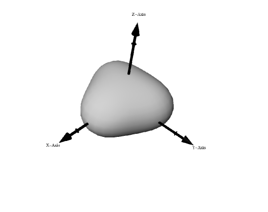
FIG. 9.: 3D representation of the coordinate location of the AH for three equal mass Misner black-holes with $\mu=1.9$

Because Brill-Lindquist initial data are more easily obtained, we have also looked for the maximal separation for Brill-Lindquist data for the same setup. The three black holes are at coordinate locations $(d,0,0)$, $(0,d,0)$ and $(0,0,d)$ in Cartesian coordinates, each with a mass of one. This means that they are in an equilateral triangle of side length $\sqrt{2}d$. The fast flow AHF, working in three dimensions with a grid spacing of $\Delta x=\Delta y=\Delta z=0.1$ and $l_{max}=12$, finds a common AH in the Brill-Lindquist data at $d=1.4$, but not at $d=1.5$ even after doubling $l_{max}$ and turning off the matrix inversion step described in [24]. We therefore estimate $d_{*}\in[1.4,1.5]$, by criteria which did give a correct bracketing for the 2 BH Misner and Brill-Lindquist data, and the 3 BH Misner data. The minimization algorithm, working with the same resolution and with $l_{max}=6$, finds the same results but is now painfully slow, taking about $25$ times longer than the fast flow on exactly the same data. This is because the black holes have been placed in such a way that there are no reflection symmetries on the coordinate planes, and this forces us to work with all $\{l,m\}$ terms in the expansion. In contrast, the 3 Misner black holes above were set up on the $x-y$ plane and had reflection symmetries both on the $x-y$ and $x-z$ planes, which allowed us to eliminate many terms from the expansion, resulting in making the minimization algorithm only $3$ times slower than the fast flow. Of course, we could have used the same configuration for the Brill-Lindquist case, but we wanted to test our finders in a situation with no special symmetries. Fig. 10 shows a comparison of the AHs found with our two 3D finders for the case $d=1.9$ using $l_{max}=6$. Again, both finders find the same surface, except close to the origin where there is a clear mismatch. This mismatch is a consequence of a lack of resolution in the spectral decomposition, and disappears if we increase $l_{max}$ to $9$ (the fast flow ‘horizon’ moves in to lie on top of the original horizon found with the minimization algorithm). Fig. 11 shows a 3D representation of the coordinate location of the same horizon. For this horizon we have found the area to be $A\sim 4.5\times 10^{2}$.

FIG. 10.: Comparison of the AHs found with our two 3D finders for three equal mass Brill-Lindquist black-holes with $d=1.4$. The solid line corresponds to the fast flow finder and the dotted line to the minimization finder.

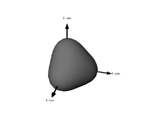
FIG. 11.: 3D representation of the coordinate location of the AH for three equal mass Brill-Lindquist black-holes with $d=1.4$

B Non time-symmetric black hole data

All the data sets considered so far are time-symmetric, $K_{ij}=0$. In this case, Eq. (4) defining marginally trapped surfaces reduces to a minimal surface equation that involves only the three-metric. Allowing $K_{ij}\neq 0$ introduces a completely new qualitative feature. While minimal surface equations have been studied a great deal in many different contexts, and while this is to a lesser extent also true in the case of non-flat metrics, general relativity with non-vanishing $K_{ij}$ introduces particular velocity and potential terms about which little appears to be known. For example, see [33] where it is pointed out that the natural generalization of the mean curvature flow method does not define a gradient flow and the area does not necessarily decrease. Nevertheless, as stated in [33], there is good reason to hope that such a flow algorithm will still converge. Here we present examples that demonstrate that all three finders are able to locate apparent horizons in black hole space times with $K_{ij}\neq 0$. Of course, $K_{ij}\neq 0$ naturally arises during evolution of the time-symmetric black hole data presented above, but we will not study evolutions in this paper.

Analytically known black hole initial data which are not time-symmetric include of course those obtained from slicing a single Kerr black hole. These data are still axisymmetric, and the horizon is a coordinate sphere. One can break the axisymmetry (of the data on a slice, not the spacetime!) by boosting the Kerr black hole in a direction not parallel to its angular momentum. This is done by writing the Kerr metric in Kerr-Schild form

$$g_{\mu\nu}=\eta_{\mu\nu}+l_{\mu}l_{\nu},$$ (28)

where $\eta_{\mu\nu}$ is flat and $l_{\mu}$ is null (with respect to both $\eta_{\mu\nu}$ and $g_{\mu\nu}$). In Cartesian coordinates $(t,x,y,z)$, one applies a Lorentz transformation to $g_{\mu\nu}$, and carries out a 3+1 split on the surface $t=0$. Explicit formulae are given in [41]. We have found the apparent horizon, and have obtained good agreement between the minimization and fast flow finders, for values for the dimensionless angular momentum of $0$, $0.5$ and $0.8$, and for the same values of the boost speed, with all combinations of these two parameters. Nevertheless, we felt that these initial data still carried too much symmetry.

In the remainder of this section we will consider conformally flat initial data for moving and spinning black holes that generalizes Brill-Lindquist data [42]. Similar tests could be carried out for a generalization of Misner type data [43]. The conformally flat line element is given by (24). The extrinsic curvature is trace free, and therefore the momentum constraint does not depend on the conformal factor. An explicit solution to the momentum constraint that characterize a single black hole with given momentum $P^{i}$, and spin $S^{i}$ is

$$K^{ij}_{PS} = \frac{3}{2r^{2}}(P^{i}n^{j}+P^{j}n^{i}-(g^{ij}-n^{i}n^{j})P^{k}n_{k})$$ (30)

$$+\frac{3}{r^{3}}(\epsilon^{ikl}S_{k}n_{l}n^{b}+\epsilon^{jkl}S_{k}n_{l}n^{i}),$$

where $n^{i}$ is the unit radial vector. Since the momentum constraint is linear in $K_{ij}$, for $N$ black holes we can solve the momentum constraint by

$$K^{ij}=\sum_{a=1}^{N}K_{PS(a)}^{ij},$$ (31)

where each term is defined by (30) with its own origin $\vec{r}_{a}$, momentum $\vec{P}_{a}$, and spin $\vec{S}_{a}$. These parameters correspond to the ADM quantities in the limit that the separation of the holes is very large.

The Hamiltonian constraint is solved by splitting a regular function, $u$, from the conformal factor, compare (27),

$$\psi=u+\sum_{i=1}^{N}\frac{m_{a}}{2\left|\vec{r}-\vec{r}_{a}\right|},$$ (32)

$$\Delta_{\delta}u+\beta(1+\alpha u)^{-7}=0,$$ (33)

where $\alpha=(\sum{m_{a}}/(2\left|\vec{r}-\vec{r}_{a}\right|))^{-1}$, $\beta=\alpha^{7}K^{ij}K_{ij}/8$, and $u\rightarrow 1$ at infinity. A key feature of the “puncture method” is that the resulting elliptic equation for $u$ can be implemented on $R^{3}$ despite the apparent singularities at the $\vec{r}_{a}$ [42].

1 One black hole data

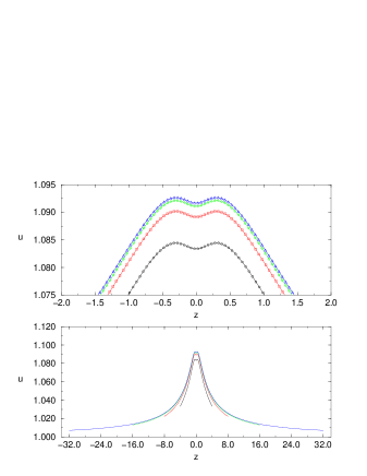
FIG. 12.: Regular part of the conformal factor, $u$, for a single black hole with $m=1$ and $\vec{P}=(0,0,1)$ for various locations of the outer boundary. While the Robin boundary condition assumes a $1/r$ fall-off, one clearly sees the influence of the $1/r^{2}$ terms.

FIG. 13.: ADM mass integral (upper curve) and pseudo Schwarzschild mass (lower curve) for a single black hole with $m=1$ and $\vec{P}=(0,0,1)$, data from the 3D solver with nested boxes and central resolution of $\Delta=0.03125$. The leftmost piece of the curves is obtained for 5 nested boxes of sizes $[-1,1]^{3}$ to $[-16,16]^{3}$, the other from 8 nested boxes of sizes $[-2,2]^{3}$ to $[-256,256]^{3}$.

First we consider a single black hole at the origin with mass $m=1$ and momentum aligned with the $z$-axis. For non-vanishing net momentum the fall-off as one approaches infinity is rather slow, and one has to place the outer boundary of the grid sufficiently far away to obtain, e.g., mass estimates close to the ADM mass (even though a Robin boundary modeling a $1/r$ fall-off in the conformal factor was used). In Fig. 12 we show the dependence of the regular piece of the conformal factor, $u$, on the location of the outer boundary for the 2D solver, $\Delta z=0.05$. Note that $u=1$ for $\vec{P}=0$. Even though $\psi$ has a pole at $r=0$, the location of the outer boundary affects the location of the apparent horizon, which in this case intersects the $z$-axis at 0.433 for the boundary at 4.0 and at 0.436 for the boundary at 32.0.

In Fig. 13 we show how two different mass indicators depend on radius for the 3D solver (we will discuss how we calculate the masses in section V below). In 3D, some sort of adaptivity is crucial for numerical efficiency. While the approach to the mass at infinity is slow, perhaps surprisingly so considering that the apparent horizon is at about $r=0.5$, note that in general there does not exist a concept of local mass that would allow one to compute the mass at infinity at finite $r$.

In Fig. 14 we show results for the 3D apparent horizon finders for a sequence of linear momenta aligned with the $z$-axis. Here we put the outer boundary at $r=16$ which appears reasonable according to Fig. 12. In order to achieve sufficient resolution near the apparent horizon, the 3D data is computed on five nested boxes with a refinement factor of 2, $[-16,16]^{3}$ to $[-1,1]^{3}$, $64^{3}$ points each, with smallest grid spacing of $2/64=0.03125$. To quantify the agreement between the two 3D finders, we give various spectral coefficients for two resolutions in Table III.

Note that with increasing momentum the apparent horizon shrinks in these coordinates. However, the surface area computed from the metric increases: for $P^{z}=0$, 1, 2, 3, 4, and 5, the surface areas divided by $16\pi$ as found by the minimization algorithm at $\Delta=0.0625$ are 1.000102, 1.19, 1.52, 1.85, 2.16, and 2.46, respectively.

Furthermore, the apparent horizon is offset from the origin in such a way that it trails the “motion” of the center (see also [44]). This, of course, is a coordinate dependent notion. For the event horizon, as opposed to the apparent horizon, one would expect that it is displaced in the direction of the momentum because an observer would find it harder to avoid falling into a black hole that is moving towards her.

The trailing of the apparent horizon seems plausible by the following argument. Note that the extrinsic curvature is odd under reversal of momentum, $K_{ij}(-P)=-K_{ij}(P)$, while the conformal factor is even, $\psi(-P)=\psi(P)$, since the extrinsic curvature enters into the Hamiltonian constraint as $K_{ij}K^{ij}$. The expansion formula (4) contains therefore an even term, $\nabla_{i}s^{i}$, where the change in $\psi$ amounts to a symmetric deformation. The remaining term $K_{ij}s^{i}s^{j}$ (since $trK=0$), is odd in $P^{i}$ and $n^{i}$. Since for $P^{i}=0$ and for concentric spheres of radius $r$, the expansion $H(r)$ has a zero at $r=1/2$ with positive slope, we expect to see the location of the horizon on the positive $z$-axis to move to smaller $z$ with increasing $P^{z}>0$. For a rigorous argument one would have to take the non-locality of the minimal surface equation into account.

The 2D results agree with the 3D results to within less than $1\%$, which would not be visible in Fig. 14. In this case the initial data is obtained from an independent numerical code in 2D and 3D. A simple test case which is independent of numerical error in the initial data can be obtained by setting $u=1$ for non-vanishing $K_{ij}$. For the 2D data one can read off that for $u=1$ the apparent horizon is almost exactly an ellipse with radius $0.495$ in the $y$-direction, $0.499$ in the $z$-direction, and an offset in the $z$-direction of $-0.061$.

FIG. 14.: Position of the apparent horizon for a single black hole at the origin with $m=1$ and linear momentum in the $z$-direction. For $P^{z}=0.0$, the AH is a sphere of radius $0.5$. For $P^{z}=1.0$, $2.0$, $\ldots$, $5.0$, the AH shrinks and is shifted towards negative $z$ (in these coordinates). In all cases we used $l_{max}=8$ and the result for the two 3D finders cannot be distinguished.

$m=0$	$64^{3}$, $\Delta=0.03125$		$32^{3}$, $\Delta=0.06250$
$l$	fast flow	minim.	fast flow	minim.
0	4.616$\times 10^{-1}$	4.616$\times 10^{-1}$	4.622$\times 10^{-1}$	4.623$\times 10^{-1}$
1	-2.601$\times 10^{-2}$	-2.602$\times 10^{-2}$	-2.624$\times 10^{-2}$	-2.615$\times 10^{-2}$
2	1.561$\times 10^{-3}$	1.560$\times 10^{-3}$	1.562$\times 10^{-3}$	1.574$\times 10^{-3}$
3	-9.020$\times 10^{-5}$	-8.749$\times 10^{-5}$	-1.251$\times 10^{-4}$	-8.437$\times 10^{-5}$
4	6.396$\times 10^{-7}$	1.571$\times 10^{-5}$	4.636$\times 10^{-5}$	4.991$\times 10^{-5}$

TABLE III.: Spectral coefficients defining the apparent horizon for a single black hole with $m=1$ and $\vec{P}=(0,0,1)$ for $l_{max}=8$.

2 Two black hole data

We consider one particular example for non-time-symmetric and non-axisymmetric black hole binary initial data. Such data was for the first time evolved through a brief merger phase as indicated by the location of the apparent horizon in [44]. Here we compare the 3D finders for the example of [44] but with a separation such that there is one common outermost marginally trapped surface already at $t=0$, Fig. 15: $m_{1}=1.5$, $m_{2}=1$, $\vec{c}_{1,2}=(0,0,\pm 0.5)$, $\vec{P}_{1,2}=(\pm 2,0,0)$, $\vec{S}_{1}=(-0.5,0.5,0)$, $\vec{S}_{2}=(0,1,1)$. There are three grids $[-12.8,12.8]^{3}$ to $[-3.2,3.2]$ with either $64^{3}$ or $128^{3}$ points each, so that the central resolution is $\Delta=0.1$ or $0.05$, respectively. Clearly, there is a very large parameter space to study, and even more interestingly, one can also study how various black hole data sets evolve through a merger, an issue that we hope to address in a future publication.

FIG. 15.: Position of the apparent horizon for a particular binary black hole initial data set that is neither time-symmetric nor axisymmetric. Results for the 3D finders for central resolution $\Delta=0.1$ and $0.05$ and for $l_{max}=6$ and $8$ are plotted on top of each other. The difference between the finders hardly shows. The momenta $\vec{P}_{a}$ are chosen such that in the $x-z$ plane the upper hole “moves” to the right, the lower to the left.

V Brill wave spacetimes

We finally turn to a rather difficult problem: determining whether or not a horizon exists, and if so, determining its location, in a numerically generated initial data set. This will be a common situation in simulations involving gravitational collapse of matter or gravitational waves. For this test, we turn to a sequence of pure wave spacetimes, of a family originally considered by Brill [45], that must be obtained numerically through solutions to the constraint equations. If the waves are strong enough, an apparent horizon must be present [46], but at what point it appears as one increases the wave strength, or where it will be located, is unknown a priori.

A Initial data

Brill’s construction starts by considering an axisymmetric metric of the form:

$$ds^{2}=\Psi^{4}\left[e^{2q}\left(d\rho^{2}+dz^{2}\right)+\rho^{2}d\phi^{2}\right].$$ (34)

Where both $q$ and $\Psi$ are functions of $\{\rho,z\}$. In order to solve for $\Psi$, we first impose the condition of time symmetry, which implies that the momentum constraints are identically satisfied. We then chose a function $q$ and solve the Hamiltonian constraint, which for the metric (34) becomes

$$\Delta_{\delta}\Psi+\frac{1}{4}\,(q_{,\rho\rho}+q_{,zz})\,\Psi=0,$$ (35)

where $\Delta_{\delta}$ is the flat space Laplacian.

The function $q$ is almost completely arbitrary, apart from the fact that it must satisfy the following boundary conditions

$$q\left|{}_{\rho=0}\right. = 0,$$ (36)

$$\partial^{n}_{\rho}q\left|{}_{\rho=0}\right. = 0\qquad\mbox{for odd $n$},$$ (37)

$$q\left|{}_{r\rightarrow\infty}\right. = O\left(r^{-2}\right).$$ (38)

Once a function $q$ has been chosen, all that is left for one to do is solve the elliptic equation (35) numerically. This can be done in a variety of ways. Here we use two independent elliptic solvers: an axisymmetric solver based on a semi-coarsening multi-grid solver, and a multi-grid fully 3D solver (Bernd Brügmann’s BAM) hooked up to the Cactus [47] code recently developed at the Albert-Einstein-Institut. Having two independent solvers with different methods, in different coordinate systems, and in different dimensions has allowed us to cross check our results and has increased our confidence in our solution of the elliptic problem.

Different forms of the function $q$ have been used by different authors [15, 48, 49, 50]. Here we will consider two such forms, the first one introduced by Eppley in his pioneering work on Brill waves in the seventies [15, 48], and the second one introduced by Holz et al. in the early nineties [49].

Before moving on to horizon finding in pure wave spacetimes, we first comment on how to calculate the gravitational mass of a given initial data set. Finding the gravitational mass is a very useful tool in testing the accuracy of our initial data. It provides us with a single number that can be easily compared for different initial data solvers and is a good indicator of the strength of a gravitational wave. For strong wave spacetimes that collapse to a black hole, the difference between the initial mass of the wave and the mass of the final black hole is a good indicator of the percentage of energy that was radiated out to infinity. We have several ways of calculating the initial mass of our spacetimes. The first method is to use the ADM mass [51]

$$M=\frac{1}{16\pi}\lim_{r\rightarrow\infty}\oint g^{ij}g^{mn}\left(g_{in,j}-g_{ij,n}\right)\sqrt{g}\;dS_{m}$$ (39)

in appropriate coordinates.

Of course, our numerical grid does not extend all the way to infinity, so in practice we evaluate the integral at a series of different finite radii and look at its behavior as $r$ increases. As it turns out, the mass calculated using Eq. (39) converges only very slowly with $r$ even for a simple Schwarzschild black hole. A better way of calculating the mass uses the fact that for large $r$ (but still small enough to be inside the computational grid) the function $q$ becomes essentially zero and the metric is conformally flat. For conformally flat metrics the ADM mass can be rewritten as [52]

$$M=-\frac{1}{2\pi}\lim_{r\rightarrow\infty}\oint\vec{\nabla}\Psi\cdot d\vec{S}.$$ (40)

Equations (39) and (40) are only equivalent in the limit of infinite radius, but it turns out that for a Schwarzschild black hole in isotropic coordinates, Eq. (40) gives in fact the correct mass at any finite radius. Since once we are in the region where $q$ is very small the metric of our Brill wave solutions approaches the Schwarzschild metric rapidly, one finds that the masses obtained by using (40) converge very fast as $r$ increases.

A final way of calculating the mass is what we call the ‘pseudo Schwarzschild mass’. This mass estimate is obtained by first finding the areal (Schwarzschild) radius $R$ of a series of coordinate spheres, finding the correspondent metric component $g_{RR}$ (averaged over the coordinate sphere) and then defining:

$$M=\frac{R}{2}\left(1-\frac{1}{g_{RR}}\right).$$ (41)

In practice we find that for the spacetimes studied below, the mass indicator (41) also converges very rapidly with $r$.

B Eppley data

Eppley considered a function $q$ of the general form [15]

$$q=a\;\frac{\rho^{2}}{1+(r/\lambda)^{n}},$$ (42)

where $a,\lambda$ are constants, $r^{2}=\rho^{2}+z^{2}$ and $n\geq 4$. Notice here that, for odd $n$ the function $q$ is not completely smooth at the origin. Nevertheless, Eppley considered mainly the particular case $\lambda=1$, $n=5$, and in order to compare with his results we will do the same here.

Before looking for horizons, we must first convince ourselves that we can solve for the conformal factor $\Psi$ correctly, that is, that we can construct good initial data. Our approach here is to solve the initial value problem independently in axisymmetry and in full 3D and compare both results with those of Eppley. In particular, we will look at the extracted masses for a sequence of solutions with increasing amplitudes $a$. For our axisymmetric initial data we have used a grid of $800^{2}$ points with a resolution of $\Delta\rho=\Delta z=0.03125$, and for the 3D data a grid of $131^{3}$ points with a resolution of $\Delta x=\Delta y=\Delta z=0.08$. In Table IV we tabulate the values of the masses that we find for different wave amplitudes. The masses that we report here as those obtained by Eppley were read off (by us) from Fig. 1 in Ref. [15] (modulo a conventional factor of 2 in the amplitude $a$) and are thus not very accurate. The error estimates for the 2D calculations were determined from the difference of the masses obtained by looking at the falloff of the conformal factor along the $z$ and $\rho$ axis.

From Table IV we can see that the masses obtained with our axisymmetric and 3D elliptic solvers agree remarkably well between themselves, but are generally different from those reported by Eppley. For low amplitudes, Eppley’s masses are lower than those that we find. For an amplitude $a\simeq 5$, Eppley’s mass and ours coincide, but for larger amplitudes Eppley’s masses grow much faster. In fact, Eppley reports that for $a\simeq 8$, the geometry pinches off (the conformal factor has a zero) and the mass becomes infinite but we see no evidence of such behavior. Since our two independent initial data solvers agree so well with each other, we are forced to conclude that there must have been something wrong in Eppley’s calculations. It must be pointed out here that Eppley makes a very strong point of trying to calculate the masses correctly, so we must conclude that the error must have been in his solution for the conformal factor. As an example of our initial data, in Fig. 16 we show the conformal factor $\Psi(\rho,z)$ for the case $a=10$.

$a$	M (2D)	M (3D)	M (Eppley)
1	$(4.8\pm 0.1)\times 10^{-2}$	$5.0\times 10^{-2}$	$(3.6\pm 0.2)\times 10^{-2}$
2	$(1.74\pm 0.02)\times 10^{-1}$	$1.8\times 10^{-1}$	$(1.1\pm.1)\times 10^{-1}$
5	$(8.83\pm 0.07)\times 10^{-1}$	$8.9\times 10^{-1}$	$(9\pm 0.5)\times 10^{-1}$
10	$3.22\pm 0.02$	3.2	-
12	$4.85\pm 0.02$	4.9	-

TABLE IV.: Masses for Brill wave initial data with a source function $q$ of the Eppley et al. type. Notice how our 2D and 3D solvers agree remarkably well between each other, but disagree with Eppley’s results.

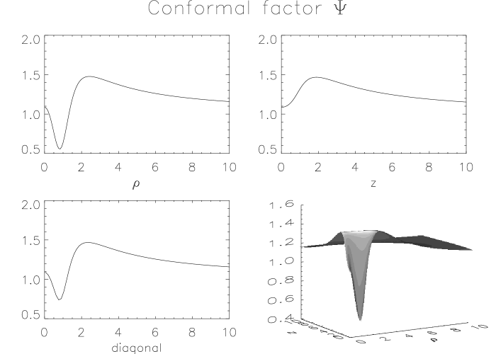
FIG. 16.: Conformal factor $\Psi(\rho,z)$ for Brill wave initial data with a source function $q$ of the Eppley type and an amplitude $a=10$.

Having constructed the initial data, we will now look for the presence of AHs. We have studied a series of solutions with increasing amplitudes with all three of our AHFs. Both our 3D finders find that an AH first appears for a critical amplitude $a_{*}\in[10.8,10.9]$. For amplitudes above $a_{*}$ we can find two horizons using the minimization algorithm (the fast flow algorithm is not designed to look for inner horizons). The 2D AHF can pin-point the value of $a*$ more precisely to $a_{*}\in[10.86,10.87]$. As we can see, the agreement in the value of $a_{*}$ is remarkable.

It is of course not enough to agree on the value of the critical amplitude above which AHs appear. We also need to compare the positions of the horizons found by the different AHFs. We have done this for many different amplitudes and found good agreement between our three AHFs. In Fig. 17 we show our standard visual test for the position of both the inner horizon and the AH for the particular case of $a=12$. Notice how in both cases the horizons coincide with zeroes of the expansion. Fig. 18 shows a comparison of the position of the AH found with the different algorithms. Again, all three finders locate the same surface. In this case we find that the area of the AH is $A\sim 1.1\times 10^{3}$. It is interesting to see whether this result agrees with the Penrose inequality [53] $16\pi M^{2}/A\geq 1$. From Table IV we see that the ADM mass in this case in $M\sim 4.85$, which implies $16\pi M^{2}/A\sim 1.07$, so the inequality is comfortably satisfied.

FIG. 17.: Position of the inner horizon and AH on the $x-z$ plane for a Brill wave initial data set using Eppley’s $q$ function with $a=12$. The solid lines are the positions of the horizons, and the dotted lines are the zeroes of the expansion $H$.

FIG. 18.: Comparison of the AHs found with our three finders for a Brill wave initial data set using Eppley’s $q$ function with $a=12$. The solid line corresponds to the 2D finder, the dotted line to the fast flow finder, and the dashed line to the minimization finder. All three lines lie on top of each other.

C Holz data

Holz et al. considered a Brill wave source function $q$ of the form

$$q=a\;\rho^{2}\;e^{-r^{2}}.$$ (43)

This form of the function $q$ is perfectly regular at the origin. An almost identical form of the function $q$ was also recently considered by Shibata [50]

$$q_{\rm Sh}={a\over 2}\;\rho^{2}\;e^{-r^{2}/2}.$$ (44)

(Note that Shibata has a different convention for $q$; this is our convention.) One can see that Shibata’s results can in fact be compared directly with those of Holz et al. because the two metrics differ only by a factor of $\sqrt{2}$ in the coordinates (and therefore also in the ADM mass), which on rescaling can be absorbed into the conformal factor (notice that multiplying the conformal factor by a constant does not affect the equation for a horizon (4) for vanishing extrinsic curvature). The strength parameter $a$ is the same in both cases.

Again, before looking for horizons, we will first test our initial data solvers by comparing the solutions of our 2D and 3D elliptic solvers with the results of Holz et al. [49, 54]. As before, the 2D initial data was calculated using $800\times 800$ grid points and a resolution of $\Delta z=\Delta\rho=0.03125$ and the 3D data using $131^{3}$ grid points with a resolution of $\Delta x=\Delta y=\Delta z=0.06$. The values of the masses we find for different wave amplitudes can be seen in Table V. Notice how the values extracted from the 2D and 3D data agree remarkably well both between themselves and with the masses of Holz et al. This gives us great confidence in the accuracy of our initial data. Fig. 19 shows in particular the conformal factor $\Psi(\rho,z)$ for the case $a=10$.

$a$	M (2D)	M (3D)	M (Holz et al.)
1	$(3.38\pm.04)\times 10^{-2}$	$3.4\times 10^{-2}$	$3.40\times 10^{-2}$
2	$(1.262\pm.009)\times 10^{-1}$	$1.3\times 10^{-1}$	$1.27\times 10^{-1}$
5	$(6.96\pm.03)\times 10^{-1}$	$7.0\times 10^{-1}$	$7.00\times 10^{-1}$
10	$2.912\pm.008$	2.9	2.91
12	$4.67\pm 0.01$	4.7	4.68

TABLE V.: Masses for Brill wave initial data with a source function $q$ of the Holz et al. type.

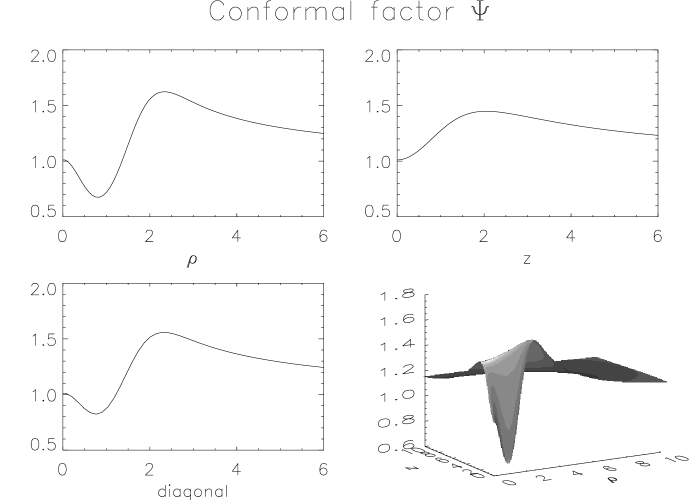
FIG. 19.: Conformal factor $\Psi(\rho,z)$ for Brill wave initial data with a source function $q$ of the Holz et al. type and an amplitude $a=10$.

Although we agree with Holz et al. on the initial data, we disagree on the AHs. Our three AHF agree among themselves, but disagree with the results reported in Ref. [49]. Holz et al. claim that an AH first appears for a critical amplitude $a_{*}=7.5$, and for larger amplitudes they can find two horizons. Our own results are qualitatively similar: a horizon first appears for a given critical amplitude, and above that we can always find two horizons. However, the value for that critical amplitude is different. Both our 3D finders indicate that $a_{*}\in[11.8,11.85]$, while the our 2D finder limits the interval to $a_{*}\in[11.81,11.82]$. Shibata, on the other hand, finds that the first AH appears for $a\sim 12$, in complete agreement with our results. The mass of the solution corresponding to the critical amplitude turns out to be $M\simeq 4.5$.

In Fig. 20 we show again our standard visual test for the position the inner and apparent horizons for the particular case of $a=12$. Fig. 21 shows a comparison of the position of the AH found with our three different finders. The area of the horizon in this case turns out to be $A\sim 1.1\times 10^{3}$. From Table V we see that in this case the ADM mass is $M\sim 4.67$, from which we find that $16\pi M^{2}/A\sim 0.997$. The Penrose inequality appears to be slightly violated, but this small violation could easily be caused by the inaccuracies in the determination of both the mass and the area.

FIG. 20.: Position of the inner horizon and AH on the $x-z$ plane for a Brill wave initial data set using Holz’ $q$ function with $a=12$. The solid lines are the positions of the horizons, and the dotted lines are the zeroes of the expansion $H$.

FIG. 21.: Comparison of the AHs found with our three finders for a Brill wave initial data set using Holz’ $q$ function with $a=12$. The solid line corresponds to the 2D finder, the dotted line to the fast flow finder, and the dashed line to the minimization finder. All three lines lie on top of each other.

VI Conclusions

In this paper we have developed a large number of test-beds for apparent horizon finding algorithms in numerical relativity, and have applied them to three algorithms of ours. There were several goals of this study. First, in preparation for studies of a wide variety of datasets it was important to verify that our algorithms are robust and that their coding is correct. As a result of this extensive testing we are now very confident that our algorithms, which had to be refined in several cases to find difficult but known horizons, are correct and robust. Second, through this study we have developed an extensive series of quantitative tests for both developing and validating future algorithms, that should be useful to the community. Third, we used these refined horizon finding algorithms to study a series of interesting black hole and gravitational wave initial data sets in preparation for numerical evolutions.

For the purpose of validating our own algorithms, we have repeated virtually all quantitative test-beds in the literature that have come to our attention. Here it was important to have some simple numbers that can be compared directly. For two of these test-beds (Brill wave data), our results disagree with the published results. We are confident that our results are the correct ones both because our three finders agree with each other, and because they agree with the literature for the other published test-beds.

At our disposal we had three apparent horizon finders, two independent ones in three space dimensions without symmetries, and one limited to axisymmetry. Both 3D finders are an integral part of the Cactus numerical relativity framework [32], so that all the test-bed data can be calculated, examined for horizons with either of the two finders, and evolved forward in time within the same code, just by changing parameters. The 2D finder was also linked up with a 2D initial data solver. While the fast flow 3D AH finder is generally much faster than the minimization routine, it was crucial for the validation process to have all three available to work on the same data. We stress that Powell’s method, which was used in the minimization algorithm, is probably not the best for the minimization, but it is common and readily available for testing the basic AH finding strategy; more sophisticated minimization algorithms could accelerate the minimization-based AH finder. The speed of the finders will be crucial in determining whether full scale numerical evolutions can be practically carried out or not, and even the present generation finders can be taxing in terms of computational time. The 2D initial data solver and apparent horizon finder, although limited to axisymmetric data, had the advantage of allowing for much higher numerical precision, thus giving us more confidence yet in our results.

We want to emphasize the importance of proper validation through test-beds, of any new algorithm, especially for analysis tools such as horizon finders for which standard techniques such as convergence tests will generally not reveal algorithm deficiencies or coding errors. Validation on simple examples with lower symmetry, or with analytically known horizons, is important but simply not sufficient. One could almost establish a variant of Murphy’s law stating that every new test-bed calculation that is in some way more generic than previous ones will reveal a new deficiency in a given finder. As AHs are not known for completely general data sets, being able to test two or three totally independent finders on the same initial data was crucial to our development process, right down to the process of eliminating typos in this paper. On the one hand, we have included some physically interesting data sets (black holes and Brill waves), on the other hand we would like to stress that for the sole purpose of testing an AHF, one can run it on data that do not obey the constraints (“bowl” spacetimes).

Finding AHs in data without symmetries remains a very difficult problem. For generic data, which are not time-symmetric, no algorithm is known to always work. Essentially, the problem is highly nonlinear, and can be made arbitrarily difficult with sufficiently “bad” data (a typical example of such behavior was discussed for the “bowl” spacetimes). In fact there may not be any “best” algorithm that is both fast and robust at the same time. Further, in different cases one algorithm may work better than another, or vice versa. For these reasons we continue to use our various AH finders to confirm results.

As an aid to future development and validation efforts, in this paper we have given simple numbers (critical separations, horizon areas and ADM masses) for families of initial data that should provide useful and quantitative testbed for other groups. However, in our opinion, validation must also include detailed comparison of the entire shape of the candidate AH with other algorithms, for data which have no symmetries at all.

The horizon finders developed and refined on these spacetimes are presently being applied to evolutions of some of these datasets. These results will be presented in future publications.

- [1] P. Anninos et al., Phys. Rev. Lett. 74, 630 (1995).
- [2] J. Libson et al., Phys. Rev. D 53, 4335 (1996).
- [3] S. Hughes et al., Phys. Rev. D 49, 4004 (1994).
- [4] R. Matzner et al., Science 270, 941 (1995).
- [5] J. Massó, E. Seidel, W.-M. Suen, and P. Walker, gr-qc/9804059. Submitted to Phys. Rev. D (1998).
- [6] S. Shapiro, S. Teukolsky, and J. Winicour, Phys. Rev. D 52, (1995).
- [7] S. W. Hawking and G. F. R. Ellis, The Large Scale Structure of Spacetime (Cambridge University Press, Cambridge, England, 1973).
- [8] E. Seidel and W.-M. Suen, Phys. Rev. Lett. 69, 1845 (1992).
- [9] G. B. Cook et al., Phys. Rev. Lett 80, 2512 (1998).
- [10] C. Gundlach and P. Walker, (1998), in preparation.
- [11] P. Anninos et al., Phys. Rev. D 50, 3801 (1994).
- [12] P. Anninos et al., Australian Journal of Physics 48, 1027 (1995).
- [13] P. Anninos et al., IEEE Computer Graphics and Applications 13, 12 (1993).
- [14] A. Čadež, Ann. Phys. 83, 449 (1974).
- [15] K. Eppley, Phys. Rev. D 16, 1609 (1977).
- [16] N. T. Bishop, Gen. Rel. Grav. 14, 717 (1982).
- [17] T. Nakamura, Y. Kojima, and K. Oohara, Phys. Lett. 106A, 235 (1984).
- [18] G. Cook and J. W. York, Phys. Rev. D 41, 1077 (1990).
- [19] A. J. Kemball and N. T. Bishop, Class. Quantum Grav. 8, 1361 (1991).
- [20] P. Anninos et al., Phys. Rev. D 58, 024003 (1998).
- [21] J. Libson, J. Massó, E. Seidel, and W.-M. Suen, in The Seventh Marcel Grossmann Meeting: On Recent Developments in Theoretical and Experimental General Relativity, Gravitation, and Relativistic Field Theories, edited by R. T. Jantzen, G. M. Keiser, and R. Ruffini (World Scientific, Singapore, 1996), p. 631.
- [22] J. Thornburg, Phys. Rev. D 54, 4899 (1996).
- [23] T. W. Baumgarte et al., Physical Review D 54, 4849 (1996).
- [24] C. Gundlach, Phys. Rev. D 57, 863 (1998), gr-qc/9707050.
- [25] M. Shibata, Phys. Rev. D 55, 2002 (1997).
- [26] J. York, in Frontiers in Numerical Relativity, edited by C. Evans, L. Finn, and D. Hobill (Cambridge University Press, Cambridge, England, 1989), pp. 89–109.
- [27] D. S. Brill and R. W. Lindquist, Phys. Rev. 131, 471 (1963).
- [28] J. Libson, in Numerical Relativity Conference, edited by P. Laguna (PUBLISHER, ADDRESS, 1993).
- [29] K. Camarda, Ph.D. thesis, University of Illinois at Urbana-Champaign, Urbana, Illinois, 1998.
- [30] K. Camarda and E. Seidel, , gr-qc/9805099. Submitted to Physical Review D.
- [31] W. H. Press, B. P. Flannery, S. A. Teukolsky, and W. T. Vetterling, Numerical Recipes (Cambridge University Press, Cambridge, England, 1986).
- [32] C. Bona, J. Massó, E. Seidel, and P. Walker, (1998), gr-qc/9804065. Submitted to Physical Review D.
- [33] K. P. Tod, Class. Quan. Grav. 8, L115 (1991).
- [34] P. Anninos et al., Phys. Rev. D 52, 2059 (1995).
- [35] C. Misner, Phys. Rev. 118, 1110 (1960).
- [36] S. G. Hahn and R. W. Lindquist, Ann. Phys. 29, 304 (1964).
- [37] L. Smarr, A. Čadež, B. DeWitt, and K. Eppley, Phys. Rev. D 14, 2443 (1976).
- [38] P. Anninos et al., Phys. Rev. Lett. 71, 2851 (1993).
- [39] P. Anninos et al., Phys. Rev. D 52, 2044 (1995).
- [40] P. Anninos, Ph.D. thesis, Drexel University, 1989.
- [41] R. A. Matzner, M. F. Huq, and D. Shoemaker, to appear in Phys. Rev. D (1998).
- [42] S. Brandt and B. Brügmann, Phys. Rev. Lett. 78, 3606 (1997).
- [43] G. B. Cook et al., Phys. Rev. D 47, 1471 (1993).
- [44] B. Brügmann, (1997), gr-qc/9708035.
- [45] D. S. Brill, Ann. Phys. 7, 466 (1959).
- [46] R. Beig and N. O’Murchadha, Phys. Rev. Lett. 66, 2421 (1991).
- [47] C. Bona, J. Carot, and J. Massó, In preparation (1998).
- [48] K. Eppley, in Sources of Gravitational Radiation, edited by L. Smarr (Cambridge University Press, Cambridge, England, 1979), p. 275.
- [49] D. E. Holz, W. A. Miller, M. Wakano, and J. A. Wheeler, in Directions in General Relativity: Proceedings of the 1993 International Symposium, Maryland; Papers in honor of Dieter Brill, edited by B. L. Hu and T. Jacobson (Cambridge University Press, Cambridge, England, 1993).
- [50] M. Shibata, Phys. Rev. D 55, 7529 (1997).
- [51] R. M. Wald, General Relativity (The University of Chicago Press, Chicago, 1984).
- [52] N. O’Murchadha and J. York, Phys. Rev. D 10, 2345 (1974).
- [53] R. Penrose, Ann. N.Y. Acad. Sci. 224, 125 (1973).
- [54] D. Holz, private communication (unpublished).