Accelerating Numerical Relativity with Code Generation: CUDA-enabled Hyperbolic Relaxation

Abstract

Next-generation gravitational wave detectors such as Cosmic Explorer, the Einstein Telescope, and LISA, demand highly accurate and extensive gravitational wave (GW) catalogs to faithfully extract physical parameters from observed signals. However, numerical relativity (NR) faces significant challenges in generating these catalogs at the required scale and accuracy on modern computers, as NR codes do not fully exploit modern GPU capabilities. In response, we extend NRPy, a Python-based NR code-generation framework, to develop NRPyEllipticGPU—a CUDA-optimized elliptic solver tailored for the binary black hole (BBH) initial data problem. NRPyEllipticGPU is the first GPU-enabled elliptic solver in the NR community, supporting a variety of coordinate systems and demonstrating substantial performance improvements on both consumer-grade and HPC-grade GPUs. We show that, when compared to a high-end CPU, NRPyEllipticGPU achieves on a high-end GPU up to a sixteenfold speedup in single precision while increasing double-precision performance by a factor of 2–4. This performance boost leverages the GPU’s superior parallelism and memory bandwidth to achieve a compute-bound application and enhancing the overall simulation efficiency. As NRPyEllipticGPU shares the core infrastructure common to NR codes, this work serves as a practical guide for developing full, CUDA-optimized NR codes.

1 Introduction

Numerical relativity (NR) plays a crucial role in the prediction, detection, and interpretation of signals observed in multi-messenger astronomy. The LIGO/Virgo/KAGRA Collaboration continues to detect compact object binary mergers, with the majority of signals consistent with binary black hole (BBH) mergers [1, 2]. The accuracy of gravitational wave (GW) models, as well as the template banks used by observatories to determine whether a GW event has been detected, heavily depends on the precision of NR simulations [3, 4, 5].

NR simulations of GW sources form the foundation for extracting parameters from observed GW signals, however, they come with a significant computational cost. This is reflected in recent high-performance computing (HPC) usage statistics which show that NR and GW physics are ranked as the third-highest user per job in recent years [6]. Looking ahead, the demand for computational resources in NR is expected to increase significantly as third-generation (3G) GW detectors, such as LISA, Cosmic Explorer, and the Einstein Telescope, become operational. These instruments will necessitate a tenfold increase in simulation accuracy [7, 8] and a significant expansion of simulation catalogs to explore new GW sources, including eccentric and high-mass-ratio compact binaries. Achieving these goals with current NR codes would entail an impractically high computational cost.

NR groups developing next–generation frameworks to meet the demands of 3G detectors face considerable challenges as advances in artificial intelligence and graphical processing unit (GPU) technologies are rapidly transforming the computing landscape. Modern HPC systems increasingly adopt heterogeneous architectures, where GPUs perform the majority of the computational workload rather than traditional central processing units (CPUs). Thus, there is an urgent need for NR frameworks capable of efficiently utilizing these architectures.

This challenge extends beyond large-scale HPC environments to consumer-grade hardware, where dedicated GPUs now offer remarkable computational performance compared to native CPUs. This is particularly relevant to our group’s proposed BlackHoles@Home volunteer computing project, which aims to harness consumer-grade hardware for generating 3G-ready BBH GW catalogs with full NR [9, 10].

BBH systems form the foundation of compact binary GW data analysis. Simulating such a system involves two basic steps: first, solving a set of elliptic partial differential equations (PDEs) to compute the initial data solution; and second, evolving this data forward in time by solving a system of hyperbolic PDEs (see e.g., [11, 12] for comprehensive reviews). Both calculations are computationally intensive, with the computational cost increasing for higher binary mass ratio and the component spins of the BHs.

Reducing the cost of 3G-ready NR BBH simulation campaigns on modern computing resources requires a deep understanding of both CPU and GPU architectures, their strengths and limitations. Typically, existing CPU-centric algorithms must be rewritten to fully utilize the latest CPU/GPU heterogeneous architectures. This presents a significant computational challenge in terms of application portability, with the goal of enabling developers to write an implementation once and have it perform efficiently across a broad spectrum of computing technologies. Ref. [13] provides a recent evaluation that compares and contrasts native codes (i.e., those developed using AMD’s HIP or NVIDIA’s CUDA) with several programming models aimed at providing application portability, including OpenMP [14], OpenACC [15], SYCL [16], RAJA [17], and Kokkos [18]. To summarize, applications that effectively leverage these programming models demonstrate promising performance across a wide range of HPC resources. Notably, Kokkos and SYCL sometimes achieve superior performance to native applications, but typically underperform.

In an effort to effectively leverage the latest HPC resources, the NR community continues to develop GPU-accelerated applications, with a primary focus on the time evolution of dynamical spacetimes. For general relativistic magnetohydrodynamic (GRMHD) simulations of isolated objects, known frameworks include AsterX [19] and GRaM-X [20], both of which use the new Einstein Toolkit [21] driver CarpetX, built on the AMReX [22] programming framework. In contrast, Kokkos has been employed to rewrite Athena++ into more portable implementations, including the multi-physics framework Parthenon [23, 24], as well as AthenaK, which supports simulations of BBHs [25] and GRMHD studies of binary and isolated neutron stars [26]. In addition, NR frameworks natively ported using CUDA include SpEC [27], optimized for simulating isolated BHs, and Dendro-GR [28], designed for BBH simulations.

An alternative to relying solely on portable programming libraries is code generation, which has become a cornerstone in both industry and NR applications [9, 29, 28, 30]. In this work, we describe the initial steps toward extending NRPy, a Python-based code-generation framework tailored for NR [9, 31], to enable the creation of highly optimized, GPU-accelerated NR applications for both consumer-grade and HPC-grade GPUs. Specifically, we focus on adapting key components to generate NRPyEllipticGPU, a CUDA-optimized version of NRPyElliptic.

In a previous work [32] (hereafter Paper I), our group introduced NRPyElliptic, an extensible elliptic solver specifically designed for NR problems and generated using NRPy. In Paper I, the capabilities of NRPyElliptic were demonstrated by solving the BBH initial data problem, a critical step in simulating GW sources. Leveraging the hyperbolic relaxation method [33], NRPyElliptic solves nonlinear elliptic PDEs using a single grid with compactified curvilinear coordinates that exploit near-symmetries of the underlying physical system. NRPyElliptic also implements an adaptive relaxation wavespeed that accelerates relaxation while maintaining the Courant-Friedrichs-Lewy (CFL) stability condition. To further enhance performance, NRPyElliptic incorporates OpenMP parallelization and advanced SIMD instruction generation.

A significant advantage of the hyperbolic relaxation approach is that it leverages the same numerical methods and code-generation infrastructure used by NR evolution codes focused on the time evolution of dynamical spacetimes. Thus, the impact of this paper is twofold: it introduces the first GPU-enabled initial data solver for BBH ID and serves as the foundation for CUDA-enabled NR evolution codes generated automatically. One such application is BlackHoles@Home, which specializes in modeling dynamical spacetimes for isolated and binary compact objects.

To this end, this study rigorously evaluates the efficiency of NRPyElliptic and NRPyEllipticGPU by analyzing their performance on both consumer-grade and HPC-grade hardware. We also demonstrate roundoff-level agreement between NRPyElliptic and NRPyEllipticGPU at double precision. While previous GPU-based NR analyses have largely focused on HPC-grade hardware, even for single-node performance [28, 20, 27], our work addresses this limitation by exploring GPU optimizations for NR applications across a broader range of hardware. This approach emphasizes both accessibility and scalability, bridging the gap between consumer-grade and high-performance systems.

The remainder of this paper is organized as follows: Sec. 2 provides a brief overview of the elliptic system used to model the two-puncture problem and the hyperbolic relaxation method employed to solve it. In Sec. 3, we describe the relevant features of the CUDA programming model, followed by a detailed overview of the numerical implementation and design decisions to extend NRPy for generating optimized CUDA code in Sec. 4. Section 5 presents our results, including agreement between NRPyEllipticGPU and NRPyElliptic to roundoff precision, additional enhancements to achieve the final benchmarks, and rigorous analysis of hardware-imposed limitations. Finally, Sec. 6 discusses the lessons learned, outlines a path toward optimized CUDA applications for dynamical spacetimes, and provides plans for future work.

2 Basic equations

Since the basic equations were introduced in detail in Paper I, we provide only a brief overview here. Using NRPyElliptic and NRPyEllipticGPU, we solve the system of equations to construct conformally flat BBH initial data. Our starting point is the $3+1$ Arnowitt-Deser-Misner (ADM) decomposition of the spacetime manifold [34, 35]:

$$ds^{2}=-\alpha^{2}dt^{2}+\gamma_{ij}(dx^{i}+\beta^{i}dt)(dx^{j}+\beta^{j}dt)\,,$$ (1)

where $\gamma_{ij}$ is the physical spatial metric, $\alpha$ is the lapse function, and $\beta^{i}$ is the shift vector. The conformal transverse-traceless (CTT) decomposition (see, e.g., [36]) reformulates the physical metric using the conformal decomposition:

$$\gamma_{ij}=\psi^{4}\tilde{\gamma}_{ij}\,,$$ (2)

where $\psi$ is a positive scalar function (the conformal factor) and $\tilde{\gamma}_{ij}$ is the conformal metric. Under the assumption of asymptotic flatness, $\tilde{\gamma}_{ij}$ is set to the flat, three-dimensional metric $\hat{\gamma}_{ij}$. For Brandt-Brügmann [37] puncture initial data considered here, this results in an analytic solution to the momentum constraint equations, leaving only the Hamiltonian constraint to solve. Because the conformal factor is singular, it is decomposed into singular and non-singular components:

$$\psi=\psi_{\rm singular}+u\,.$$ (3)

Substituting this into the Hamiltonian constraint, the equation for the non-singular function $u$ becomes:

$$\hat{\nabla}^{2}u+\frac{1}{8}\tilde{A}_{ij}\tilde{A}^{ij}(\psi_{\rm singular}+u)^{-7}=0\,,$$ (4)

where $\hat{\nabla}$ is the covariant derivative compatible with the flat background metric $\hat{\gamma}_{ij}$ and $\tilde{A}_{ij}$ is the conformal trace-free extrinsic curvature. We solve this equation using the hyperbolic relaxation method, which recasts Eq. (4) as a system of coupled first-order (in time) PDEs:

$$\partial_{t}u = v-\eta u\,,$$

$$\partial_{t}v = c^{2}\left[\tilde{\nabla}^{2}u+\frac{1}{8}\tilde{A}_{ij}\tilde{A}^{ij}(\psi_{\rm singular}+u)^{-7}\right]\,,$$ (5)

where $\eta$ is a damping factor and $c$ is the wave speed. In the steady-state regime, where $\partial_{t}u=\partial_{t}v=0$, the solution of Eqs. 5 coincides with that of the original system.

Formulated as a hyperbolic PDE, this approach to solving elliptic PDEs completely avoids the need to recast the PDEs in matrix form or to linearize them. Further, being hyperbolic, it adopts the same infrastructure as a traditional NR evolution code, making implementation even easier. However, this convenience usually comes at a cost: hyperbolic relaxation methods are relatively inefficient for solving elliptic PDEs, requiring that constant-speed relaxation waves cross the numerical grid many times.

As described in Paper I, we address this inefficiency by adjusting the wave speed $c$ in Eqs. 5 to be proportional to the local grid spacing and by utilizing NRPy’s SinhSymTP coordinate system. These tools provide a nonuniform grid that is denser near the punctures and grows exponentially toward the outer boundary while ensuring that the CFL constraint is satisfied throughout the relaxation. Cumulatively, these modifications significantly accelerate relaxation waves toward the outer boundary thereby drastically reducing the relaxation time, bringing this method to the level of state-of-the-art elliptic solvers.

Having established the foundational equations and the numerical method used to solve them, we next outline the core requirements for adapting NR codes like NRPyElliptic to GPUs. Recognizing that the reader, likely a numerical relativist, may not be familiar with the intricacies of CUDA programming, we begin by providing an overview of the CUDA programming model.

3 Overview of the CUDA programming model

To leverage CUDA-enabled GPUs effectively for NR applications, it is essential to understand the fundamental components and principles of the CUDA programming model. To do so, we will adopt the standard CUDA coding naming conventions throughout this text such that references to device (host) code refer to code executed by the GPU (CPU). Developed by NVIDIA, CUDA is a parallel computing platform that enables the use of NVIDIA GPUs for general-purpose computations, significantly accelerating tasks that benefit from parallel processing.

At the core of CUDA are Streaming Multiprocessors (SMs), which are analogous to CPU cores, but designed to handle thousands of lightweight threads concurrently. While a typical CPU may have a handful of powerful cores optimized for sequential processing and complex tasks, an SM contains multiple smaller cores optimized for high-throughput parallelism. This architecture is supported by a hierarchical memory system, similar to the multi-level cache hierarchy in CPUs, designed to optimize data access and hide latency.

Each generation and class of CUDA-enabled device has an associated compute capability which corresponds to intrinsic features and specifications that are available in NVIDIA’s C Programming Guide [38]. A critical insight into a GPU’s capabilities (see section 5.4.1 of [38]) is the number of arithmetic instructions (for a given precision) that can be performed per clock cycle per SM. Understanding these specifications is important to determine the maximum theoretical performance of an application on a given GPU, a point that will be revisited in Sec. 5.

A fundamental concept in CUDA is the Single Instruction, Multiple Threads (SIMT) model, which shares similarities with the Single Instruction, Multiple Data (SIMD) model used in CPUs, but offers greater flexibility. For CUDA-enabled devices, threads are grouped into units called warps (typically 32 threads) that must execute the same instruction. However, each thread in a warp can follow its own control flow which can result in threads within a warp taking a different execution path (a situation known as thread divergence). In this case, performance can degrade substantially. Therefore, minimizing thread divergence is crucial for optimizing performance, analogous to avoiding branch mis-predictions and ensuring uniform execution in SIMD operations on CPUs.

Within an SM, threads are organized into blocks, which determines the number of active threads per SM, the number of registers available per thread, and the tiling strategy for looping over grid data. Blocks are further organized into a grid, which represents the 3D domain of the problem and is used to distribute the workload across the GPU. To maximize the computational performance of each thread, it is essential to ensure each thread has the maximum available cache resources. For the GPUs used here, this corresponds to 255 32-bit registers per thread with a block size not to exceed 256 threads.

There are four key types of memory in CUDA pertinent to this work: global, shared, registers, and constant. Global memory offers larger storage capacity for GPUs, and is analogous to the main system memory (RAM) accessible by all CPU cores, though with significantly higher bandwidth and significantly lower capacity. Much like RAM, accessing global memory is typically much slower than accessing caches or registers. Efficient use of global memory often requires organizing data so that consecutive threads access contiguous memory locations, maximizing data throughput and minimizing latency, similar to optimizing memory access patterns in CPU applications to leverage cache lines effectively.

Shared memory is located at the SM level and is accessible by all threads within the same block. It is significantly faster than global memory and is ideal for storing data that multiple threads need to access frequently, thereby reducing the need to fetch data from slower global memory repeatedly. This is analogous to how CPU cores share caches to speed up data access among threads, however, unlike CPUs shared memory is explicitly managed by the programmer.

Each thread has its own set of registers, providing the fastest access to data. This is analogous to CPU registers, which store frequently accessed variables for quick computation. However, similar to CPUs, the number of registers is limited, so efficient usage is crucial to avoid spilling to slower memory and incurring performance penalties.

Constant memory is a specialized read-only memory area cached on the GPU, with a small cache size of $\sim 64{\rm KB}$. Constant memory is optimized for scenarios where all threads read the same data simultaneously, much like broadcast instructions in CPU SIMD operations, with latency comparable to an L1 cache. While the allocation of constant memory must be known at compile time, the stored data can be modified in host code at runtime. The constness comes from being immutable in device code. Additionally, constant data can be implicitly stored in the constant cache by the compiler if the compiler is able to determine that a variable is constant at compile time and will fit into the cache limits.

Within the CUDA API, execution on the GPU is achieved using Global kernels. Global kernels are central to CUDA programming as they are the mechanism for the host to launch code on the device and for defining a parallelization strategy. As such, they must be declared and launched in a specific manner:

⬇

// Kernel function declaration (e.g., in a header file)

__global__ global_kernel(MyDataType data);

// Kernel launch by the host (e.g., in the main function)

global_kernel<<<Grid, Block, sm, stream>>>(data);

where, in reverse order, stream is an optional argument that specifies the kernel to execute using a specific CUDA stream; sm is the optional bytesize of shared memory arrays which allows for dynamic specification; Block is a device organizational structure that represents the number of threads per block; and Grid specifies the number of logical Blocks required to complete the calculation. Organizing threads and blocks effectively is essential for maximizing parallel efficiency, much like optimizing thread distribution and workload balance across CPU cores to prevent bottlenecks and ensure efficient utilization.

It is important to note that execution of global kernels by the host are done asynchronously. Specifically, after the kernels are launched by the host, the host will continue executing the next instructions until an explicit synchronization is encountered. The execution of additional global kernels by the host will then be tasked to the GPU scheduler and executed in the order they are tasked.

Data transfer between the host and device occurs over the PCI-Express bus, introducing latency and bandwidth limitations. To mitigate these issues, CUDA provides features such as pinned (page-locked) memory and asynchronous data transfers. Pinned memory ensures faster data transfers by preventing the operating system from moving the memory to slower storage, such as disk or swap space—a process called “paging.” By locking the memory in RAM, it guarantees that the data remains immediately accessible for transfers. This approach is similar to reserving specific memory regions in CPU applications to ensure consistent and rapid access.

CUDA also supports streams, which is an additional layer of parallelization that allows multiple kernels or memory operations to be executed concurrently. By assigning independent tasks to separate streams, computation and communication operations can be executed asynchronously, improving overall performance by allowing the CPU and GPU to work concurrently without waiting for data transfers to complete.

Finally, CUDA offers intrinsics, which are specialized functions that provide optimized performance for specific mathematical operations [[, see Sec. 13.2 in]]nvidia_cpg. These intrinsics allow for more efficient computations by leveraging hardware-specific instructions, enabling higher performance without relying solely on compiler optimizations. This is akin to using SIMD intrinsics functions for CPU code that map directly to specific assembly instructions, allowing one to exploit processor-specific features for performance gains. Incorporating CUDA intrinsics can lead to significant speedups in compute-intensive parts of NR applications, given NR calculations often involve complex mathematical operations that can be challenging for compilers to effectively optimize.

3.1 Key Considerations for Numerical Relativity Applications

When adapting NR codes to run on CUDA-enabled GPUs, several important factors must be addressed to achieve optimal performance, drawing parallels to optimization strategies employed on CPU architectures:

• Memory Management: NR simulations often involve large datasets and complex data structures. Efficiently organizing data to take advantage of shared and constant memory can significantly reduce access times and improve performance, much like optimizing data layout in CPU caches to enhance cache locality and minimize cache misses.

• Parallelization Strategy: The inherent parallelism in NR problems must be mapped effectively to the GPU’s architecture. This involves decomposing the computational domain and ensuring that the workload is evenly distributed across threads to prevent bottlenecks, analogous to distributing tasks evenly across CPU cores to maximize parallel efficiency and avoid core idle times.

• Minimizing Divergence: Conditional operations in NR algorithms can lead to thread divergence within warps, thereby reducing performance. Designing kernels to minimize these divergences ensures that all threads within a warp execute instructions efficiently, similar to minimizing branch instructions and ensuring consistent execution paths in CPU SIMD operations to prevent pipeline stalls.

• Data Transfer Optimization: Reducing the frequency and volume of data transfers between the host and device is crucial. Techniques such as overlapping computation with data transfers and utilizing pinned memory can help mitigate the impact of PCI-Express latency.

• Scalability: Ensuring that the code scales well with increasing problem sizes and fully utilizes the computational power of modern GPUs, including both consumer-grade and HPC-grade hardware, is vital for future-proofing NR simulations. This is comparable to designing CPU applications that scale efficiently with the number of cores and leverage advanced CPU features to maintain performance as hardware evolves.

Addressing these considerations enables NR applications to fully exploit the computational capabilities of CUDA-enabled GPUs. In the following section, we will discuss how these are tackled in the extension of NRPy to generate high-performance NR applications.

4 Adapting NRPy for CUDA code generation

Building on these foundational principles of the CUDA programming model and its application to NR, we now explore the extension of NRPy to generate CUDA-optimized NR codes. Our primary focus is on NRPyEllipticGPU, which is the first application to fully leverage these new features. We begin by providing an Algorithmic Overview of NRPyEllipticGPU, including its hybrid CPU+GPU design and the structural inheritance from NRPy’s native infrastructure, BlackHoles@Home. Next, we discuss how NRPyEllipticGPU addresses each of the five key considerations when adapting NR applications to GPUs, as discussed in the previous section. Finally, we present the complete NRPyEllipticGPU algorithm (Alg. 1), which we reference throughout this section.

Adapting NRPy for generating CUDA-enabled applications involves a reimagination of the code generation process such that the key abstractions such as the grid and mathematical calculations are preserved while the underlying implementation is optimized for GPU execution by leveraging the unique features of the CUDA programming model. Although the underlying extensions are generic and reusable, we use NRPyEllipticGPU as an illustrative example. NRPy’s BlackHoles@Home infrastructure, used by NRPyEllipticGPU/NRPyElliptic and detailed in [9, 32], is particularly well-suited for GPU acceleration for three main reasons:

1. Memory-Efficient, Multipatch Design: BlackHoles@Home’s native support for curvilinear coordinates minimizes memory usage, making even consumer-grade GPUs with only 8–14GB of memory sufficient for nontrivial NR simulations.

2. Flattened Grid Arrays: By storing all grid functions in a single flat array, NRPy reduces pointer overhead and balances GPU register usage more effectively than if each grid function were separately allocated.

3. Large, Compute-Intensive Kernels: NRPy naturally generates sizable kernels involving finite-difference stencils, which GPUs handle efficiently thanks to their high memory bandwidth and SIMT execution model.

In addition, we extend NRPy to leverage a hybrid approach to allow the host to handle small, sequential tasks while offloading compute-heavy sections to the device. In NRPyEllipticGPU, this prevents performance degradation from excessive host–device data transfers and optimizes the overall runtime. Specifically, the main GPU-intensive tasks in Alg. (1) include computing right-hand sides (RHS), Hamiltonian constraint residuals (H), Runge-Kutta (RK) stages, and boundary conditions (BC). Tasks that are inherently sequential or require minimal computation, such as identifying boundary points between grids and writing checkpoints, remain on the CPU side. As noted in lines 8–9 and steps (a)–(c) of Alg. (1), this approach ensures that if GPU scheduling and synchronization overhead outweigh the benefit of parallelizing a small task, the task will be done on host and only the data needed will be transferred to the device.

4.1 Memory Management

Effective memory management is crucial when porting NR codes to GPUs. Since NR problems often involve large arrays of data, NRPy’s decision to flatten grid functions into a single array reduces the overhead of pointer dereferencing and helps maintain ample registers for arithmetic operations. Beyond this foundational step, two additional strategies help manage memory efficiently:

• Measuring Memory Requirements Early: Since the average consumer GPUs today offer as little as 8 GB of memory, it’s essential to determine if the problem size fits within the available GPU memory. In NRPy applications, the total memory footprint is allocated up front at runtime, thereby providing quick feedback on whether a chosen problem size fits on the GPU. This is particularly important because high-end consumer cards may have up to ${\sim}14$ GB of RAM, while HPC-grade GPUs can exceed 40 GB. Consequently, the memory limit remains a major concern for large NR applications.

• Use of Constant Memory: CUDA constant memory is leveraged for read-only, frequently accessed data. This is especially beneficial for small arrays of numerical parameters or precomputed constants (e.g., Runge-Kutta coefficients), which the compiler can store in a fast cache shared by all threads.

In NRPy, we leverage constant memory in two ways. First, we explicitly store constant parameters as (e.g. number of grid points, grid spacing, dt, relaxation wavespeed) which are copied as needed to the device prior to launching a GPU kernel. In practice this storage ends up being arrays of length nstreams. Second, we leverage the compiler’s ability to implicitly store numerical constants (e.g. Runge-Kutta coefficients) in constant memory. This is achieved by using SymPy and NRPy’s advanced CSE algorithms to aggressively identify numerical constants and move them to const (or static constexpr for C++ applications) variable definitions. The added benefit is that expensive instructions to compute rational constants can be moved to compile time and efficiently accessed by all threads.

4.2 Parallelization Strategy

Under the CUDA paradigm, parallelization involves launching one or more kernels over a grid of thread blocks, each block containing multiple threads. NRPy translates standard CPU loops into global CUDA kernels by mapping loop indices to thread and block indices. This seamless translation is facilitated by the flattened array representation, which simplifies kernel logic.

By default, NRPy uses a block size of $(32,\,\mathbf{NGHOSTS},\,1)$, where 32 is the typical warp size and $\mathbf{NGHOSTS}$ is the radius of the finite-difference stencil. Although this choice is not always optimal for every kernel, it balances performance across a variety of possible finite-difference orders (2–12). Tests with profiler-recommended block sizes (e.g., using NVIDIA Nsight Compute) showed marginal speedups, emphasizing that current compute limitations often arise from hardware constraints and double-precision demands.

Although CUDA supports dynamic allocation of on-chip shared memory, we do not currently rely on it for NRPyEllipticGPU. Tests that included shared memory strategies did not significantly improve performance for the compute-heavy kernels, which are currently limited by double-precision hardware throughput rather than memory bandwidth. Specifically, using NVCC, we observed that using shared memory optimized kernels would reduce the number of generated instructions without a measurable speedup for the compute-bound parts of the code. It also introduced significant code complexity in NRPy for generating such kernels. However, shared memory may prove more beneficial for future multi-patch evolution codes (e.g., BSSN) or other multi-kernel workflows. We plan to revisit shared memory strategies when exploring those more complex applications.

4.3 Minimizing Divergence

In CUDA’s SIMT execution model, threads within a warp execute instructions in lockstep. If threads within the same warp follow different control flows (branching), performance degrades due to warp divergence. NRPy uses two strategies to mitigate this:

• Uniform Branching: Where possible, conditionals are designed so that threads in a warp make consistent decisions.

• Predication and Simplified Conditionals: For short conditional regions, code is predicated to avoid divergent branching altogether.

These strategies mirror NRPy’s CPU-oriented SIMD optimizations and help maintain high throughput on GPUs.

4.4 Data Transfer Optimization

Data transfers between the host and device occur over relatively slow buses, making them a potential bottleneck if not handled efficiently. NRPy addresses this in the following ways:

• Hybrid CPU+GPU Work Distribution: By performing only large, data-intensive parts of the simulation on the GPU, NRPyEllipticGPU avoids repeated data transfers for small workloads. Alg. (1) outlines our approach, which ensures that tasks remain on the CPU if the overhead of transferring data to the GPU and scheduling a kernel would exceed any potential speedup.

• Pinned Memory and Asynchrony: NRPy allocates pinned (page-locked) memory on the host using cudaMallocHost, facilitating faster, asynchronous host–device transfers. Critical housekeeping tasks (e.g., computing the grid $L^{2}$ norm of the Hamiltonian constraint violations) are overlapped with data transfers so that the GPU remains busy while data is being moved.

• CUDA Streams: Multiple CUDA streams can be used to schedule concurrent kernel executions and asynchronous copies. In multi-patch or multi-grid contexts, streams help overlap computations for different patches, although the best performance gain is achieved when each kernel is sufficiently large to hide scheduling overheads. By default, we set the number of streams to $\texttt{nstreams}=3$, one per coordinate direction, but we find only a marginal speed-up using more than one stream and an insignificant speedup for $\texttt{nstreams}>3$. In other scenarios or more compute heavy kernels, streams may prove to be more beneficial.

4.5 CUDA Intrinsics

A key advantage of NRPy is its ability to generate explicitly vectorized code, combining common subexpression elimination (CSE) with hardware intrinsics to aggressively fuse arithmetic operations. This becomes increasingly important for NR applications as the mathematical expressions get so long that it can be challenging for compilers to optimize the code effectively. By default, NRPy detects long arithmetic expressions in finite-difference stencils and replaces repeated operations with corresponding CUDA intrinsics where appropriate, reducing the total number of floating-point operations in the final compiled kernel. Intrinsics in the CUDA setting (e.g., __dmul_rn, __dadd_rn, or __fma_rn) ultimately results in fewer instructions being executed and more efficient cache usage, thus improving performance and reducing rounding errors .

Algorithm 1 NRPyEllipticGPU Driver: Host (Device) denotes a task performed on the CPU (GPU). The most computationally expensive operations are boldfaced: H, RHS, BC, and RK.

1:Host: Initialize global array of CUDA streams.

2:Device: Set up uniformly sampled coordinate 1D arrays $x^{i}$, transfer to host.

3:Device: Precompute reference metric components and derivatives.

4:Host: Initialize “inner” and “outer” boundary conditions [9, 32] containers, transfer to device.

5:Device: Allocate storage for Runge-Kutta stages and constant source terms grid functions.

6:Host: Allocate storage for diagnostics stored on the entire grid.

7:Device: Set initial conditions and compute constant source terms.

8:while $t\leq t_{\rm final}$ do

9:  Device: Compute residual (H; left-hand side of Eq. 4)

10:  Host: Request asynchronous data transfer from device for diagnostics.

11:  Device: Compute residual $L^{2}$ norm.

12:  while Runge-Kutta step incomplete do

13:   Device: Evaluate right-hand sides (RHS) of Eqs. 5.

14:   Device: Apply boundary conditions [32] (BC) to evolved variables $u$ and $v$.

15:   Device: Perform Runge-Kutta substep (RK) update.

16:  end while

17:  Host: Compute timestep.

18:  Host: Check alternate stop condition based on the $L^{2}$ norm of residual.

19:end while

20:Synchronize device and host.

21:Free device and host allocated storage.

22:Program terminates.

4.6 Scalability

The flattened array layout and well-structured kernel design allow NRPy-based codes to scale effectively across GPUs ranging from consumer-grade (NVIDIA RTX series) to HPC-grade (A100, L40, etc.). Since each GPU has more streaming multiprocessors (SMs) than a CPU has cores, the large and compute-heavy kernels generated by NRPy often achieve near-peak bandwidth usage, as shown in Sec. 5. This approach ensures that as problem sizes grow or as more advanced hardware becomes available, NRPyEllipticGPU remains a viable solution for numerically challenging NR applications.

4.7 Complete NRPyEllipticGPU Driver Algorithm

The complete NRPyEllipticGPU driver workflow is detailed in Alg. (1). The solver begins by allocating and initializing data structures on both the host (CPU) and device (GPU). It then enters the primary relaxation loop, which executes on the GPU, while the host manages auxiliary tasks. Convergence checks and diagnostic computations are performed asynchronously to optimize performance. Once a stopping criterion is satisfied, NRPyEllipticGPU synchronizes operations and deallocates resources on both the host and device before terminating the execution.

With these core optimizations in place, we now turn to the performance benchmarks and accuracy studies of NRPyEllipticGPU, which confirm both its consistency with the CPU-based NRPyElliptic code and its ability to deliver high performance across various GPU platforms.

5 Results

Table 1: Specifications of the hardware tested, including a consumer-grade PC and a standard node in the Falcon cluster. Each Falcon node contains two CPUs.

System	Model	DRAM		TDP (W)
		Capacity (GB)	Bandwidth (GB/s)
Desktop-CPU	Ryzen 9 5950x	$64$	$42.7$	105
Desktop-GPU	RTX3080	$12$	$912.0$	320
Falcon-CPU	Xeon E5-2695v4	$128$	$76.8$	120
Falcon-GPU	L40	$40$	$864.0$	300

Using the hardware described in Sec. 5.1, we present four studies. First, Sec. 5.2 compares NRPyEllipticGPU and NRPyElliptic to verify that our CUDA implementation achieves numerical accuracy consistent with the trusted OpenMP version, agreeing at roundoff levels. Second, Sec. 5.3 evaluates the weak algorithmic scaling of the core computational kernels introduced in Alg. (1): RHS (Right-Hand Side), BC (Boundary Conditions), RK (Runge-Kutta substeps), and H (Hamiltonian Constraint). Third, Sec. 5.4 investigates the impact of intrinsics on performance and accuracy. Finally, Sec. 5.5 examines the scalability of NRPy-generated GPU kernels for HPC systems and BlackHoles@Home’s multipatch grids, demonstrating their suitability for larger-scale simulations.

5.1 Hardware Overview

Except for Fig. 5, all results were obtained on a single consumer desktop (see Tab. 1 for specifications). This desktop includes an AMD Ryzen 9 5950x (CPU) and a NVIDIA RTX3080 (GPU) with compute capability $8.6$. Each implementation employs $10$th-order finite-difference stencils. Comparisons with NRPyElliptic use its highly optimized, OpenMP-parallelized version, which benefits from NRPy’s SIMD optimizations. Here we restrict OpenMP to one thread per physical core, as no noticeable performance benefit was measured when using hyperthreads since the available cache per thread is reduced.

5.2 Consistency Study: Roundoff-Level Agreement between NRPyElliptic and NRPyEllipticGPU

To establish consistency, we verify that solutions from NRPyEllipticGPU and NRPyElliptic agree at roundoff levels. Figure 1 displays the relative difference in the solution $u$ along grid points nearest to the $y$-axis. Red squares represent the comparison halfway through relaxation ($t_{\rm mid}$), while blue squares depict it at the end of relaxation ($t_{\rm end}$). Both solutions are computed on a $128{\times}128{\times}16$ grid using NRPy’s SinhSymTP coordinate system (see Paper I for details). The solutions show excellent agreement, with a norm of approximately $9\text{\times}{10}^{-13}$, indicating minimal, roundoff-level discrepancies. As we’ll find in Sec. 5.4, enabling intrinsics can further reduce these discrepancies.

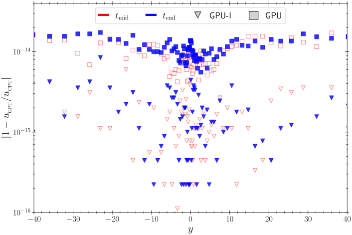
Figure 1: Solution comparison between NRPyElliptic and NRPyEllipticGPU halfway through relaxation (red) and at the end of relaxation (blue). Triangle (square) markers denote generating NRPyEllipticGPU with (without) CUDA intrinsics.

5.3 Efficiency Study: Roofline Analysis

Having established consistency with the trusted NRPyElliptic code, we evaluate the efficiency of NRPyElliptic and NRPyEllipticGPU on the CPU and GPU, respectively. For profiling, we use Likwid 5.3 on the CPU and NVIDIA Nsight Compute 2022.3.0.0 on the GPU, focusing on the four most computationally intensive kernels: RHS, H, RK, and BC.

5.3.1 Roofline Analysis Methodology

For our roofline analysis, we plot the number (billions) of floating-point operations per second (GFLOP/s) versus the arithmetic intensity (AI; FLOP/Byte). The lower “roof” represents memory bandwidth, and the upper “roof” corresponds to the theoretical peak FLOP/s. Although our analysis focuses on main memory bandwidth (DDR/GDDR), its principles extend to various cache levels. It is important to emphasize that AI is strongly tied to the memory demand of a kernel as well as the complexity of the calculation. Stated differently, a sufficiently complex calculation can outweigh the memory access latency if there is enough work to be performed.

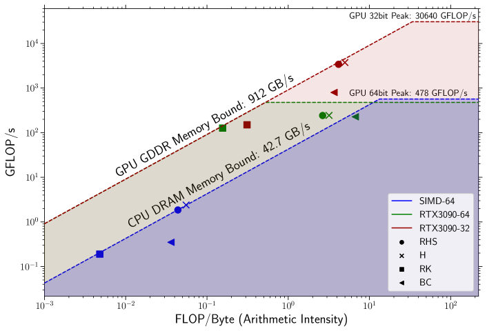
Figure 2: Roofline comparison of the vectorized (SIMD) CPU version of NRPyElliptic and the accelerated NRPyEllipticGPU (GPU) codes. Here we plot the data for the RHS (Right-Hand Side), H (Hamiltonian Constraint), RK (Runge-Kutta substeps), and BC (Boundary Conditions) kernels. CPU metrics were obtained using Likwid 5.3, while GPU metrics were obtained using NVIDIA Nsight Compute 2022.3.0.0.

5.3.2 Performance Metrics and Observations

Figure 2 compares CPU (dashed blue for double precision) and GPU (dashed red for single precision, dashed green for double precision) performance on a $512{\times}512{\times}64$ grid in SinhSymTP coordinates. Here we denote the kernel performance for the RHS (circles), H (crosses), RK (squares), and BC (triangles). The first observation to note is that the CPU’s double-precision peak performance slightly surpasses that of the GPU. Additionally, the GPU’s single-precision peak is approximately 64x higher than its double-precision peak, reflecting the optimization of consumer-grade GPUs for single-precision performance. Finally, the elbows of the roof (i.e., the transition to the upper roof) denote the threshold from an algorithm that is memory bound (above the roofs) to one that is compute bound (below the roofs).

Focusing first on the CPU results (blue markers), we find that all kernels are heavily memory bound, resulting in low AI ($10^{-3}\lesssim{\rm AI}<10^{-1}$), with RK being the lowest. Conversely, GPU kernels generally achieve higher AI ($10^{-1}\lesssim{\rm AI}<10^{1}$), with GFLOP/s near the GPU’s peak double precision performance. The GPU kernels are primarily compute-bound except for RK, which remains memory-bound due to its minimal arithmetic workload. The GPU’s higher AI is largely attributed to its 21x greater memory bandwidth and the GPU’s ability to significantly hide latency by having considerably more active threads executing instructions each clock cycle. Furthermore, by moving as much information to compile time regarding the memory layout, access patterns, and efficient use of CUDA constant cache, the CUDA compiler is able to effectively optimize memory accesses.

To gain further insight into the discrepancies between single and double precision calculations on the GPU, it is important to first identify the inherit limitations of devices with compute capability 8.6. Specifically, these devices can perform at most 2 double-precision calculations per clock cycle, while up to 128 single-precision calculations can be performed per clock cycle (see section 5.4.1 of [38]). Therefore, for an optimized kernel with sufficiently high complexity (i.e., ${\rm AI}>10^{1}$), the achieved FLOP/s in single-precision should be 64x more than for double precisions.

To this end, we have implemented strong floating-point typing into NRPy to enable the generation of optimized single-precision executables. Here we have leveraged this capability to generate the single-precision version of NRPyEllipticGPU and have included the associated roofline results in Fig. 2. We find that the AI is roughly constant with the achieved FLOP/s being ${\sim}10{\rm x}$ higher than for double-precision, at which point the H and RHS kernels become memory bound. Therefore, the single-precision kernels are not able to achieve the theoretical maximum speedup of 64x.

5.3.3 Comparative Analysis with Other GPU-Enabled NR Codes

Direct comparisons with other GPU-enabled NR codes are nontrivial; however, we contrast our roofline analysis against results from previous literature for the CUDA port of Dendro-GR [28] and the early Kokkos port of Athena, K-Athena [23]. Specific roofline observations include:

• Dendro-GR: In Fig. 14 of Ref. [28], the AI for octant-to-patch operations ($m_{i}$) aligns well with our results. However, their RHS kernel exhibits ${\rm AI}<10^{0}$ even on a higher-end NVIDIA A100 (compute capability $8.0$), largely associated with cache misses and register spillage inherent to solving the full system of Einstein’s equations in 3+1 form, which are far more complex than Eqs. (5).

• K-Athena: In Fig. 2 of Ref. [23], the reported AI for the 3D linear wave problem is approximately 1.5 on an NVIDIA V100 (compute capability 7.0), which is only ${\sim}2{\rm x}$ higher than the reported CPU AI.

We note that both references use data center grade GPUs, where each SM is capable of computing $32$ double-precision calculations per clock cycle as compared to the GPUs used in this work which are restricted to $2$ double-precision calculations per clock cycle.

Overall, we conclude that NRPyEllipticGPU demonstrates high efficiency on consumer-grade GPUs, with the potential for further speedups when used with modern data center-grade GPUs with considerably higher double-precision throughput.

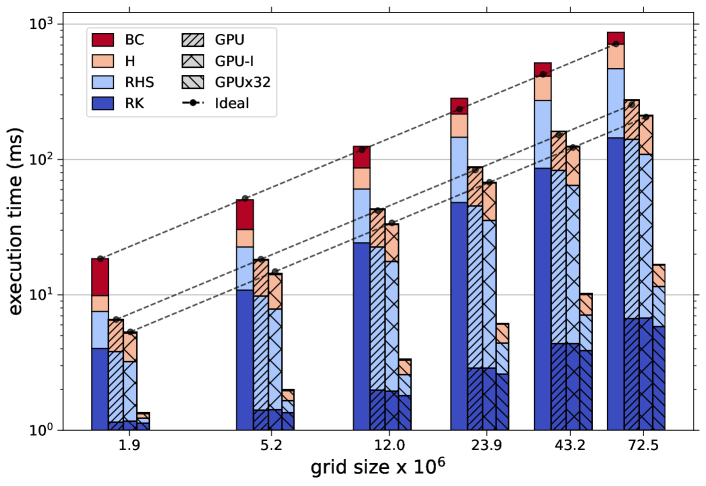
Figure 3: For each bar, we show the execution time for a single call to each kernel, not the entire program runtime, for increasing grid sizes. We compare the NRPyElliptic CPU code (no hatch marks) against NRPyEllipticGPU without CUDA intrinsics (GPU), NRPyEllipticGPU with CUDA intrinsics (GPU-I), and NRPyEllipticGPU using single precision (GPU$\times$32). Dashed lines denote approximate ideal weak scaling.

5.4 Impact of Intrinsics

We next assess the effect of intrinsics, i.e., specialized CUDA instructions (e.g., fused multiply-add), that can reduce total instructions, thus improving efficiency. To quantify this, we compare the executed instruction counts and categories using NVIDIA Nsight Compute, both without (“No intrinsics”) and with (“Intrinsics”) CUDA intrinsics when generating the RHS kernel.

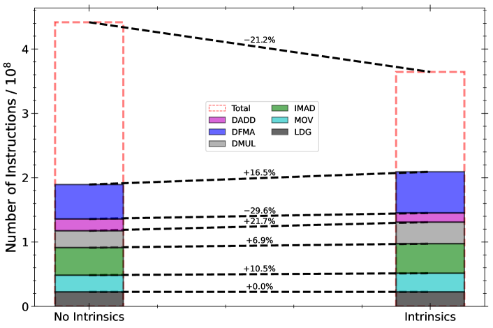
Figure 4: Instruction distribution for the NRPyEllipticGPU RHS kernel, comparing the code port without intrinsics (No intrinsics) to one using CUDA intrinsics (Intrinsics). The “Total Instructions” bar shows the overall reduction in instruction count.

Figure 4 demonstrates that enabling intrinsics reduces the total executed instructions by approximately 21. This is largely attributed to the ${\sim}\qty{16.5}{}$ increase in DFMA (Double-Precision Fused Multiply-Add), a key component to reducing DADD (Double-Precision Add) operations by ${\sim}\qty{29.6}{}$. We further find a ${\sim}\qty{10.5}{}$ increase in MOV operations, which implies more efficient cache use during calculations. Enabling intrinsics in the H and RHS kernels further improves total runtime by 1.3x and 1.2x, respectively, compared to the No-Intrinsics NRPyEllipticGPU port and by ${\sim}4{\rm x}$ relative to NRPyElliptic (Fig. 3, GPU-I). However, when energy usage is estimated based on TDP-per-unit-speedup, the energy efficiency gains are more modest, yielding only a 1.3x improvement over NRPyElliptic .

An unexpected advantage of adopting intrinsics is slightly improved numerical agreement with NRPyElliptic as shown in Fig. 1 (triangles), where the discrepancy between solutions decreases by $10^{1}$–$10^{2}$. Thus, enabling intrinsics enhances both performance and accuracy.

5.5 Scalability

The flattened array layout and structured kernel design enable NRPyEllipticGPU to scale effectively across single GPUs, from consumer-grade (e.g., RTX series) to HPC-grade (e.g., A100, L40). With significantly more streaming multiprocessors (SMs) than CPU cores, GPUs allow NRPyEllipticGPU to saturate bandwidth for its larger kernels, as demonstrated in Sec. 5.3. We conclude that the CUDA kernels emitted by NRPy provide a highly performant foundation for NRPyEllipticGPU and pave the way for full NR evolution codes that better exploit GPU capabilities.

5.5.1 Performance on HPC Hardware

To gauge the performance gap between consumer and HPC hardware, we repeat the analysis shown in Fig. 2 and Fig. 3 on a single node of the retired Idaho National Laboratory cluster, Falcon, the results of which are illustrated in Fig. 5. Each Falcon node features two Xeon E5-2695v4 CPUs and an L40 GPU (see Tab. 1 for specifications). While the L40 offers higher theoretical performance, practical gains over the RTX3080 are limited to ${\sim}$15. We contribute this, potentially surprising, minimal increase in performance to their compute capability (8.9 for the L40 and 8.6 for the RTX3080), which implies they are both limited to two double-precision calculations per clock cycle [38], thus further emphasizing the hardware imposed limitations to the measured performance.

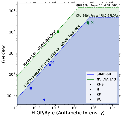
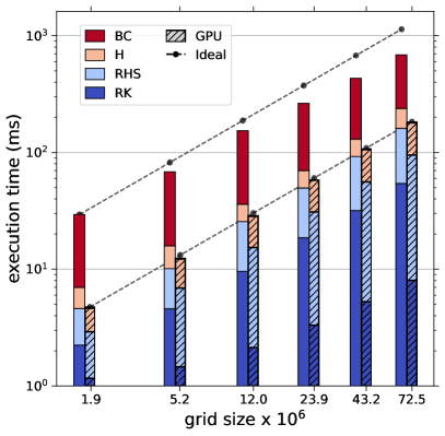
Figure 5: Same as Fig. 2 (Left) and Fig. 3 (Right), but using the HPC Falcon cluster. The L40 has compute capability 8.9, which is still limited to two double-precision operations per clock cycle.

5.5.2 Multiple, Independent Patches Performance

Finally, in preparation for BlackHoles@Home multipatch grids, we performed identical relaxations on multiple independent grids in parallel using NRPyElliptic and NRPyEllipticGPU with $1\leq N\leq 7$ identical grids of size $128{\times}128{\times}16$, the smallest grid size ($1.3\text{\times}{10}^{6}$) used in Fig. 3. Here we have disabled diagnostic outputs during runtime except when saving the solution at the end of the calculation.

In Fig. 6 (left) we illustrate the ratio of the total runtime for a given number of grids to the total runtime for a single grid, where results for NRPyElliptic are in blue and results for NRPyEllipticGPU with intrinsics using $1$ (N) CUDA streams are shown in orange (green). Here we find that NRPyEllipticGPU scales nearly as $\mathcal{O}(N)$, whereas NRPyElliptic exhibits scaling closer to $\mathcal{O}(N^{1.5})$.

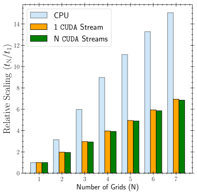
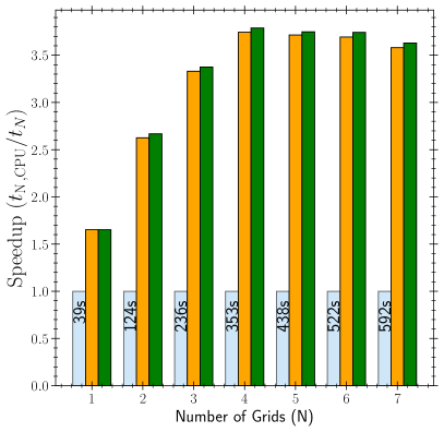
Figure 6: Left: Total execution time ($t_{N}$) for $N$ grids, normalized by the single-grid runtime ($t_{1}$). NRPyElliptic results (blue) increase faster than the nearly linear NRPyEllipticGPU results using $1$ CUDA stream (orange) or N CUDA streams (green). Right: Overall GPU speedup compared to NRPyElliptic.

To gauge the relative speedup of NRPyEllipticGPU vs NRPyElliptic, we illustrate in Fig. 6 (right) the speedup as a function of the number of grids. We define the speedup as the total CPU runtime to solution for a given number of grids ($t_{\rm N\,,CPU}$) normalized by $t_{\rm N}$ for CPU and GPU execution. For the CPU, the speedup bar is always $1$, included for clarity and to annotate $t_{N\,,\rm CPU}$ for each CPU bar. For NRPyEllipticGPU, the measured speedup ranges from a minimum of 1.65x for a single coarse grid to a maximum of 3.79x with four grids, averaging 3.23x. This behavior suggests the scheduler is likely saturated at four grids, with the decline for ${N}>4$ likely due to launch latency overhead.

These benchmarks were repeated using $\texttt{nstreams}\in\left\{1\,,3\,,N\right\}$ to evaluate the benefits of additional CUDA streams. Using $\texttt{nstreams}=N$ is approximately 1.2x faster than $\texttt{nstreams}=1$ and at most 0.5x faster than using $\texttt{nstreams}=3$, regardless of $N$. The marginally maximum benefit occurs when $\texttt{stream}=N=4$, reinforcing that saturation of the launch scheduler at $N\sim 4$ significantly contributes to overall latency. Additionally, the grid coarseness results in a less expensive kernel, which may limit the ability to fully benefit from multiple streams.

These findings demonstrate the ability of GPUs to manage multiple independent patches while minimizing latency through efficient CUDA scheduling. Such scalability is crucial for leveraging GPUs for large-scale NR simulations. For these tests, synchronizations between the host and device are minimal, limited to data transfers for disk storage. Therefore, these results represent an important upper performance bound, as the patches are independent and require no inter-patch data sharing.

6 Conclusions & Future Work

In this work, we extended the Python-based NRPy code generation framework to generate optimized CUDA-enabled programs, marking a major step in adapting NR codes to use GPU architectures. As a first example of this improved capability, we developed NRPyEllipticGPU, the first GPU-accelerated elliptic solver aimed at solving the BBH initial value problem. Using NRPy’s flexible code generation for various coordinate systems, NRPyEllipticGPU retains the adaptability of its CPU-based predecessor, NRPyElliptic, supporting Cartesian-like, spherical-like, cylindrical-like, and bispherical-like geometries.

Our tests show that NRPyEllipticGPU produces results that match NRPyElliptic at roundoff levels, ensuring accurate solutions for NR simulations. By leveraging the GPU’s SIMT model and high-bandwidth memory, NRPyEllipticGPU shifts key calculations from being memory-bound on CPUs to being compute-bound on GPUs. This optimization leads to large performance gains, with NRPyEllipticGPU running about 4x faster on an NVIDIA RTX3080 GPU using double precision. On HPC-grade hardware (NVIDIA L40), performance increases by only $\sim 15\%$ compared to the RTX3080, reflecting the shared limitation of two double-precision operations per clock cycle for both architectures. Switching to single precision provides roughly a 16x speedup for the more computationally intensive kernels, rather than the theoretical 64x, as the application becomes memory bound. This suggests that NRPyEllipticGPU using double precision would be significantly more performant on, e.g. an NVIDIA V100 or A100, which are capable of $32$ or $64$ double precision calculations per clock cycle, respectively.

A roofline analysis supports these observations, demonstrating that NRPyEllipticGPU’s kernels can achieve up to a $10^{2}$-fold improvement in arithmetic intensity (AI) compared to CPU versions. This improvement arises from more efficient memory access patterns, lower data transfer overhead, and carefully tuned CUDA kernels (see Fig. 2). Adding CUDA intrinsics—specialized instructions that fuse arithmetic operations—reduces instruction counts by approximately 21 for certain kernels (e.g., H and RHS), resulting in an additional $1.2$–$1.3{\times}$ speedup over the non-intrinsic GPU version (and about $4\times$ relative to NRPyElliptic). Intrinsics also improve numerical agreement with NRPyElliptic by one to two orders of magnitude.

NRPyEllipticGPU’s algorithmic design minimizes communication overhead between the host and device, limiting synchronizations to diagnostics during the hyperbolic relaxation procedure. Local coordinate storage and asynchronous data transfers ensure smooth data movement within single-grid applications. These optimizations have provided valuable insights for future work. Extending these methods to multi-patch simulations and solving Einstein’s equations in full will require tackling similar challenges, along with managing the greatly increased register pressure associated with larger kernels, which could significantly impact performance.

To gauge the efficiency of NRPyEllipticGPU, we have compared with other GPU-enabled NR frameworks, such as Dendro-GR and K-Athena, which indicates that NRPyEllipticGPU achieves competitive performance despite its focus on single-grid applications and simpler systems of PDEs. We note that direct comparison is not possible, especially since these frameworks support adaptive mesh refinement and more complex physics. However, NRPyEllipticGPU’s ability to handle computationally demanding tasks with reduced memory bottlenecks underscores the benefits of NRPy’s automatic code generation for specialized high-performance kernels and its potential for future multi-grid applications.

Looking ahead, our NRPy-based CUDA extensions are designed to integrate seamlessly into full NR evolution codes (e.g., BlackHoles@Home), unlocking the potential of both consumer- and HPC-grade GPUs for large-scale BBH simulations. Several complex tasks to achieve these goals include efficiently parallelizing interpolation between grids and finding an optimal GPU kernel adaptation for the BSSN system which has proven to be challenging [28]. Additionally, this work provides a template that can be used to extend NRPy to additional architectures (e.g. HIP), thus removing the restriction to CUDA enabled devices. Collectively, these developments could enable the crowd-sourced generation of extensive GW catalogs and facilitate the exploration of multi-messenger phenomena within NR. Finally, we also plan to incorporate GPU acceleration into our Charm++-capable version of BlackHoles@Home, enabling efficient use of multi-GPU setups and HPC resources. This extension would open up regions of BBH parameter space that are beyond the reach of consumer-grade hardware. It will also address challenges such as efficient load balancing and support for heterogeneous architectures.

In summary, the development and validation of NRPyEllipticGPU underscore the potential of GPU acceleration for NR applications and the power of code generation using NRPy. With significant performance gains and robust accuracy, NRPyEllipticGPU underscores how modern computing architectures and automatic code generation can meet the increasing demands of NR simulations. As the field continues to evolve toward GPU-dominated systems, the methods and tools presented here will play a pivotal role in advancing gravitational-wave astrophysics and multi-messenger astronomy.

Code Availability

The latest version of NRPyEllipticGPU is available at:
https://github.com/samueltootle/nrpy_gpu_arxiv.

References

- [1] R. Abbott “GWTC-2.1: Deep extended catalog of compact binary coalescences observed by LIGO and Virgo during the first half of the third observing run” In Phys. Rev. D 109.2, 2024, pp. 022001 DOI: 10.1103/PhysRevD.109.022001
- [2] R. Abbott “GWTC-3: Compact Binary Coalescences Observed by LIGO and Virgo during the Second Part of the Third Observing Run” In Phys. Rev. X 13.4, 2023, pp. 041039 DOI: 10.1103/PhysRevX.13.041039
- [3] V. Gayathri et al. “Eccentricity estimate for black hole mergers with numerical relativity simulations” In Nature Astron. 6.3, 2022, pp. 344–349 DOI: 10.1038/s41550-021-01568-w
- [4] J. Lange “Parameter estimation method that directly compares gravitational wave observations to numerical relativity” In Phys. Rev. D 96.10, 2017, pp. 104041 DOI: 10.1103/PhysRevD.96.104041
- [5] B. P. Abbott “Directly comparing GW150914 with numerical solutions of Einstein’s equations for binary black hole coalescence” In Phys. Rev. D 94.6, 2016, pp. 064035 DOI: 10.1103/PhysRevD.94.064035
- [6] “ACCESS Resource Metrics (XMOD)” Accessed: 2024-09-07, Available at: https://xdmod.access-ci.org/
- [7] Michael Pürrer and Carl-Johan Haster “Gravitational waveform accuracy requirements for future ground-based detectors” In Phys. Rev. Res. 2.2, 2020, pp. 023151 DOI: 10.1103/PhysRevResearch.2.023151
- [8] Deborah Ferguson, Karan Jani, Pablo Laguna and Deirdre Shoemaker “Assessing the readiness of numerical relativity for LISA and 3G detectors” In Phys. Rev. D 104.4, 2021, pp. 044037 DOI: 10.1103/PhysRevD.104.044037
- [9] Ian Ruchlin, Zachariah B. Etienne and Thomas W. Baumgarte “SENR/NRPy+: Numerical Relativity in Singular Curvilinear Coordinate Systems” In Phys. Rev. D 97.6, 2018, pp. 064036 DOI: 10.1103/PhysRevD.97.064036
- [10] Zachariah B. Etienne “Improved moving-puncture techniques for compact binary simulations” In Phys. Rev. D 110.6, 2024, pp. 064045 DOI: 10.1103/PhysRevD.110.064045
- [11] Thomas W. Baumgarte and Stuart L. Shapiro “Numerical Relativity: Solving Einstein’s Equations on the Computer”, 2010
- [12] Eric Gourgoulhon “3+1 formalism and bases of numerical relativity”, 2007 arXiv:gr-qc/0703035
- [13] Joshua H. Davis et al. “Taking GPU Programming Models to Task for Performance Portability” In arXiv e-prints, 2024, pp. arXiv:2402.08950 DOI: 10.48550/arXiv.2402.08950
- [14] OpenMP Architecture Review Board “OpenMP Application Program Interface Version 5.0”, 2018 URL: https://www.openmp.org/wp-content/uploads/OpenMP-API-Specification-5.0.pdf
- [15] J. A. Herdman et al. “Achieving Portability and Performance through OpenACC” In 2014 First Workshop on Accelerator Programming using Directives, 2014, pp. 19–26 DOI: 10.1109/WACCPD.2014.10
- [16] Istvan Z. Reguly “Evaluating the performance portability of SYCL across CPUs and GPUs on bandwidth-bound applications” In Proceedings of the SC ’23 Workshops of The International Conference on High Performance Computing, Network, Storage, and Analysis, SC-W ’23 Denver, CO, USA: Association for Computing Machinery, 2023, pp. 1038–1047 DOI: 10.1145/3624062.3624180
- [17] David A. Beckingsale et al. “RAJA: Portable Performance for Large-Scale Scientific Applications” In 2019 IEEE/ACM International Workshop on Performance, Portability and Productivity in HPC (P3HPC), 2019, pp. 71–81 DOI: 10.1109/P3HPC49587.2019.00012
- [18] Christian R. Trott et al. “Kokkos 3: Programming Model Extensions for the Exascale Era” In IEEE Transactions on Parallel and Distributed Systems 33.4, 2022, pp. 805–817 DOI: 10.1109/TPDS.2021.3097283
- [19] Jay V. Kalinani “AsterX: a new open-source GPU-accelerated GRMHD code for dynamical spacetimes” In arxiv, 2024 arXiv:2406.11669 [astro-ph.HE]
- [20] Swapnil Shankar et al. “GRaM-X: a new GPU-accelerated dynamical spacetime GRMHD code for Exascale computing with the Einstein Toolkit” In Class. Quant. Grav. 40.20, 2023, pp. 205009 DOI: 10.1088/1361-6382/acf2d9
- [21] “Einstein Toolkit home page” http:einsteintoolkit.org
- [22] Weiqun Zhang et al. “AMReX: A Framework for Block-Structured Adaptive Mesh Refinement” In Journal of Open Source Software 4.37, 2019, pp. 1370 DOI: 10.21105/joss.01370
- [23] Philipp Grete, Forrest W Glines and Brian W O’Shea “K-athena: a performance portable structured grid finite volume magnetohydrodynamics code” In IEEE Transactions on Parallel and Distributed Systems 32.1 IEEE, 2020, pp. 85–97
- [24] Philipp Grete et al. “Parthenon – a performance portable block-structured adaptive mesh refinement framework” In arXiv e-prints, 2022, pp. arXiv:2202.12309 DOI: 10.48550/arXiv.2202.12309
- [25] Hengrui Zhu et al. “Performance-Portable Numerical Relativity with AthenaK” In arxiv, 2024 arXiv:2409.10383 [gr-qc]
- [26] Jacob Fields et al. “Performance-Portable Binary Neutron Star Mergers with AthenaK” In arxiv, 2024 arXiv:2409.10384 [astro-ph.HE]
- [27] Adam G. M. Lewis and Harald P. Pfeiffer “GPU-accelerated simulations of isolated black holes” In Class. Quant. Grav. 35.9, 2018, pp. 095017 DOI: 10.1088/1361-6382/aab256
- [28] Milinda Fernando et al. “A GPU-accelerated AMR solver for gravitational wave propagation” In International Conference for High Performance Computing, Networking, Storage and Analysis, 2022 DOI: 10.5555/3571885.3571984
- [29] Carlos Palenzuela et al. “A Simflowny-based finite-difference code for high-performance computing in numerical relativity” In Class. Quant. Grav. 35.18, 2018, pp. 185007 DOI: 10.1088/1361-6382/aad7f6
- [30] Adam J. Peterson, Don Willcox, Philipp Mösta and Phillip Moesta “Code generation for AMReX with applications to numerical relativity” In Class. Quant. Grav. 40.24, 2023, pp. 245013 DOI: 10.1088/1361-6382/ad0b37
- [31] “NRPy+’s webpage” http://nrpyplus.net/
- [32] Thiago Assumpcao, Leonardo R. Werneck, Terrence Pierre Jacques and Zachariah B. Etienne “Fast hyperbolic relaxation elliptic solver for numerical relativity: Conformally flat, binary puncture initial data” In Phys. Rev. D 105.10, 2022, pp. 104037 DOI: 10.1103/PhysRevD.105.104037
- [33] Hannes R. Rüter, David Hilditch, Marcus Bugner and Bernd Brügmann “Hyperbolic Relaxation Method for Elliptic Equations” In Phys. Rev. D 98.8, 2018, pp. 084044 DOI: 10.1103/PhysRevD.98.084044
- [34] Richard L. Arnowitt, Stanley Deser and Charles W. Misner “Dynamical Structure and Definition of Energy in General Relativity” In Phys. Rev. 116, 1959, pp. 1322–1330 DOI: 10.1103/PhysRev.116.1322
- [35] Richard L. Arnowitt, Stanley Deser and Charles W. Misner “The Dynamics of general relativity” In Gen. Rel. Grav. 40, 2008, pp. 1997–2027 DOI: 10.1007/s10714-008-0661-1
- [36] Gregory B. Cook “Initial data for numerical relativity” In Living Rev. Rel. 3, 2000, pp. 5 DOI: 10.12942/lrr-2000-5
- [37] Steven Brandt and Bernd Bruegmann “A Simple construction of initial data for multiple black holes” In Phys. Rev. Lett. 78, 1997, pp. 3606–3609 DOI: 10.1103/PhysRevLett.78.3606
- [38] “NVIDIA: CUDA C Programming Guide webpage” https://docs.nvidia.com/cuda/cuda-c-programming-guide/
- [39] Charles R. Harris et al. “Array programming with NumPy” In Nature 585.7825 Springer ScienceBusiness Media LLC, 2020, pp. 357–362 DOI: 10.1038/s41586-020-2649-2
- [40] Pauli Virtanen et al. “SciPy 1.0: Fundamental Algorithms for Scientific Computing in Python” In Nature Methods 17, 2020, pp. 261–272 DOI: 10.1038/s41592-019-0686-2
- [41] Aaron Meurer et al. “SymPy: symbolic computing in Python” In PeerJ Computer Science 3, 2017, pp. e103 DOI: 10.7717/peerj-cs.103
- [42] J. D. Hunter “Matplotlib: A 2D graphics environment” In Computing in Science & Engineering 9.3 IEEE COMPUTER SOC, 2007, pp. 90–95 DOI: 10.1109/MCSE.2007.55