BSSN equations in spherical coordinates without regularization: vacuum and non-vacuum spherically symmetric spacetimes

Abstract

Brown $[$Phys. Rev. D 79, 104029 (2009)$]$ has recently introduced a covariant formulation of the BSSN equations which is well suited for curvilinear coordinate systems. This is particularly desirable as many astrophysical phenomena are symmetric with respect to the rotation axis or are such that curvilinear coordinates adapt better to their geometry. However, the singularities associated with such coordinate systems are known to lead to numerical instabilities unless special care is taken (e.g., regularization at the origin). Cordero-Carrión will present a rigorous derivation of partially implicit Runge-Kutta methods in forthcoming papers, with the aim of treating numerically the stiff source terms in wave-like equations that may appear as a result of the choice of the coordinate system. We have developed a numerical code solving the BSSN equations in spherical symmetry and the general relativistic hydrodynamic equations written in flux-conservative form. A key feature of the code is that it uses a second-order partially implicit Runge-Kutta method to integrate the evolution equations. We perform and discuss a number of tests to assess the accuracy and expected convergence of the code, namely a pure gauge wave, the evolution of a single black hole, the evolution of a spherical relativistic star in equilibrium, and the gravitational collapse of a spherical relativistic star leading to the formation of a black hole. We obtain stable evolutions of regular spacetimes without the need for any regularization algorithm at the origin.

I Introduction

The 3+1 formulation of Einstein equations originally proposed by Nakamura Nakamura87 and subsequently modified by Shibata-Nakamura Shibata95 and Baumgarte-Shapiro Baumgarte99 , which is usually known as the BSSN formulation, has become the most widespread used formulation in the numerical relativity community. This is due to its stability properties, and to the developments associated with gauge conditions and the puncture method which have proved essential to perform accurate and long-term stable evolutions of spacetimes containing black holes (BHs) Campanelli06 ; Baker06 .

The main drawback of the BSSN formulation in its original form resides in the fact that it is particularly tuned for Cartesian coordinates, since this involves dynamical fields which are not true tensors and assumes that the determinant of the conformal metric is equal to one. Brown Brown09 addressed this issue and introduced a covariant formulation of the BSSN equations which is well suited for curvilinear coordinate systems. This is particularly desirable as many astrophysical phenomena are symmetric with respect to the rotation axis (e.g., accretion disks) or are such that spherical coordinates adapt better to their geometry (e.g., gravitational collapse).

However, the singularities associated with the curvilinear coordinate systems are a known source of numerical problems. For instance, one problem arises because of the presence of terms in the evolution equations that behave like $1/r$ near the origin $r=0$. Although on the analytical level the regularity of the metric ensures that these terms cancel exactly, on the numerical level this is not necessarily the case, and special care should be taken in order to avoid numerical instabilities. A similar problem appears also near the axis of symmetry in axisymmetric systems if curvilinear coordinate systems are used.

Several methods have been proposed to handle the issue of regularity in curvilinear coordinates. One possible approach is to rely on a specific gauge choice (i.e., the polar$/$areal gauge) Bardeen83 ; Choptuik91 , but it has the obvious limitation of restricting the gauge freedom which is one of the main ingredients for successful evolutions with the BSSN formulation. An alternative method is to apply a regularization procedure. One such regularization methods, presented by Rinne05 , enforces both the appropriate parity regularity conditions and local flatness in order to achieve the desired regularity of the evolution equations. Such method has the advantage that it allows a more generic gauge choice, and has been explored by Alcubierre05 ; Ruiz08 ; Alcubierre10 who have performed several numerical simulations of regular spacetimes in spherical and axial symmetry. In particular, in Alcubierre10 , the authors applied a regularization algorithm to the BSSN equations in spherical symmetry. A disadvantage of such a regularization algorithm is that it is not easy to implement numerically both conditions simultaneously, and it requires the introduction of auxiliary variables as well as finding their evolution equations. This is an obstacle if one wants to perform 3D simulations of regular spacetimes with spherical coordinates.

Therefore, one would ideally like to use a numerical scheme that is able to integrate in time a system of equations like the BSSN, in curvilinear coordinates (with or without symmetries), without the burden of regularization in order to achieve the desired stability and robustness. Implicit or partially implicit methods are used to deal with systems of equations that require a special numerical treatment in order to achieve stable evolutions. The origin of the numerical instabilities may be diverse. Stiff source terms in the equations can lead to the development of numerical instabilities, and with some choices of the coordinate system, source terms may introduce factors which can be numerically interpreted as stiff terms (e.g., $1/r$ factors due to spherical coordinates close to $r=0$ even when regular data is evolved). Recently, partially implicit Runge-Kutta (PIRK) methods for wave-like equations in spherical coordinates have been successfully applied CC12 to the hyperbolic part of Einstein equations in the Fully Constrained Formulation FCF .

The first steps through the rigorous derivation of the PIRK methods will appear in CC-Toro and a detailed description of the methods and their properties will be derived in a forthcoming paper CC-PIRK . Motivated by these results, we have developed a numerical code solving the BSSN equations in spherical symmetry and the general relativistic hydrodynamics equations written in flux-conservative form Banyuls97 . The code uses a second-order PIRK method to integrate the evolution equations in time, and we do not apply any regularization scheme at the origin. This approach has the additional advantages that it imposes no restriction at all on the gauge choice (one can therefore use the moving puncture gauge) and no special care should be taking in the transition between a regular spacetime and that containing a singularity as it happens in the gravitational collapse of a star to a BH.

The paper is organized as follows. The formulation of Einstein equations, including the implementation of the puncture approach and gauge conditions, along with the formulation of the general relativistic hydrodynamic equations is briefly presented in Sec. II. Sec. III gives a short description of the PIRK method used, while Sec. IV describes the numerical implementation. Sec. V discusses numerical simulations of a pure gauge wave, the evolution of a single BH, the evolution of spherical relativistic stars in equilibrium, and the gravitational collapse of a spherical relativistic star leading to the formation of a BH. A summary of our conclusions is given in Sec. VII. We use units in which $c=G=M_{\odot}=1$. Greek indices run from 0 to 3, Latin indices from 1 to 3, and we adopt the standard convention for the summation over repeated indices.

II Basic equations

We next give a brief overview of the formulation for the system of Einstein and hydrodynamic equations as it has been implemented in the code.

II.1 BSSN equations in spherical symmetry

A reformulation of the ADM system, the BSSN formulation Nakamura87 ; Shibata95 ; Baumgarte99 , has been implemented to solve Einstein equations. In particular, we solve the BSSN equations in the special case of spherical symmetry. We refer to Alcubierre10 for a detailed description of the equations.

Under this symmetry condition the spatial line element is written as

$$dl^{2}=e^{4\chi}[a(r,t)\,dr^{2}+r^{2}\,b(r,t)\,d\Omega^{2}],$$ (1)

where $d\Omega^{2}$ is the solid angle element, $d\Omega^{2}=d\theta^{2}+\sin^{2}\theta d\varphi^{2}$, $a(r,t)$ and $b(r,t)$ are the metric functions, and $\chi$ is the conformal factor defined as

$$\chi=\frac{1}{12}{\rm{ln}}(\gamma/\hat{\gamma}),$$ (2)

where $\hat{\gamma}$ is the determinant of the conformal metric. The conformal metric relates to the physical one by

$$\hat{\gamma}_{ij}=e^{-4\chi}\gamma_{ij}.$$ (3)

Initially, the determinant of the conformal metric fulfills the condition that it equals the determinant of the flat metric in spherical coordinates $\mathring{\gamma}_{ij}$ (i.e. $\hat{\gamma}(t=0)=\mathring{\gamma}=r^{4}\sin^{2}\theta$). Moreover, we follow the so called “Lagrangian” condition $\partial_{t}{\hat{\gamma}}=0$ (i.e. choosing $\sigma=1$ in Eqs. (2.4), (2.6), (2.7), (2.16) and (2.17)). The evolution equation for the conformal factor takes the form

$$\partial_{t}\chi=\beta^{r}\partial_{r}\chi+\sigma\hat{\nabla}_{m}\beta^{m}-\frac{1}{6}\alpha K,$$ (4)

$K$ being the trace of the extrinsic curvature, $\alpha$ the lapse function, and

$$\hat{\nabla}_{m}\beta^{m}=\partial_{r}\beta^{r}+\beta^{r}\left(\frac{\partial_{r}(ab^{2})}{2ab^{2}}+\frac{2}{r}\right)$$ (5)

the divergence of the shift vector $\beta^{i}$. The evolution equations for the conformal metric components are:

$$\partial_{t}a=\beta^{r}\partial_{r}a+2a\partial_{r}\beta^{r}-\frac{2}{3}\sigma a\hat{\nabla}_{m}\beta^{m}-2\alpha aA_{a},$$ (6)

$$\partial_{t}b=\beta^{r}\partial_{r}b+2b\frac{\beta^{r}}{r}-\frac{2}{3}\sigma b\hat{\nabla}_{m}\beta^{m}-2\alpha bA_{b},$$ (7)

where $\hat{A}_{ij}$ is the traceless part of the conformal extrinsic curvature, and

$$A_{a}\equiv\hat{A}^{r}_{r}\;,\;\;\;\;\;\;A_{b}\equiv\hat{A}^{\theta}_{\theta}.$$ (8)

Note that as $\hat{A}_{ij}$ is traceless $A_{a}+2A_{b}=0$. The evolution equation for $K$ is:

$$\partial_{t}K =\beta^{r}\partial_{r}K-\nabla^{2}\alpha+\alpha(A_{a}^{2}+2A_{b}^{2}+\frac{1}{3}K^{2})$$

$$+4\pi\alpha(E+S_{a}+2S_{b}),$$ (9)

with the matter source terms measured by the Eulerian observers given by

$$E = n_{\mu}n_{\nu}T^{\mu\nu},$$

$$j_{i} = -\gamma_{i\mu}n_{\nu}T^{\mu\nu},$$

$$S_{ij} = \gamma_{i\mu}\gamma_{j\nu}T^{\mu\nu},$$ (10)

$T^{\mu\nu}$ being the stress-energy tensor for a perfect fluid, which is written as a function of the rest-mass density $\rho$, the specific enthalpy $h$, the pressure $P$ and the fluid 4-velocity $u^{\mu}$,

$$T^{\mu\nu}=\rho hu{{}^{\mu}}u^{\nu}+Pg^{\mu\nu},$$ (11)

and

$$S_{a}\equiv S^{r}_{r}\;,\;\;\;\;\;\;S_{b}\equiv S^{\theta}_{\theta}.$$ (12)

The Laplacian of the lapse function with respect to the physical metric is given by

$$\nabla^{2}\alpha =\frac{1}{\alpha e^{4\chi}}\bigg{[}\left.\partial^{2}_{r}\alpha-\partial_{r}\alpha\left(\frac{\partial_{r}a}{2a}-\frac{\partial_{r}b}{b}-2\partial_{r}\chi-\frac{2}{r}\right)\right].$$ (13)

Next, the evolution equation for the independent component of the traceless part of the conformal extrinsic curvature, $A_{a}$, is given by

$$\partial_{t}A_{a} =\beta^{r}\partial_{r}A_{a}-\left(\nabla^{r}\nabla_{r}\alpha-\frac{1}{3}\nabla^{2}\alpha\right)+\alpha\left(R^{r}_{r}-\frac{1}{3}R\right)$$

$$+\alpha KA_{a}-16\pi\alpha(S_{a}-S_{b}),$$ (14)

where $R^{r}_{r}$ is the mixed radial component of the Ricci tensor, $R$ its trace, and $\nabla^{r}\nabla_{r}\alpha$ is written as

$$\nabla^{r}\nabla_{r}\alpha=\frac{1}{\alpha e^{4\chi}}\left[\partial^{2}_{r}\alpha-\partial_{r}\alpha\left(\frac{\partial_{r}a}{2a}+2\partial_{r}\chi\right)\right].$$ (15)

Finally, the evolution equation for $\hat{\Delta}^{r}$, the radial component of the additional BSSN variables $\hat{\Delta}^{i}=\hat{\gamma}^{mn}\hat{\Delta}^{i}_{mn}$ with $\hat{\Delta}^{a}_{bc}=\hat{\Gamma}^{a}_{bc}-\mathring{\Gamma}^{a}_{bc}$, is given by

$$\partial_{t}\hat{\Delta}^{r} =\beta^{r}\partial_{r}\hat{\Delta}^{r}-\hat{\Delta}^{r}\partial_{r}\beta^{r}+\frac{1}{a}\partial^{2}_{r}\beta^{r}+\frac{2}{b}\partial_{r}\left(\frac{\beta^{r}}{r}\right)$$

$$+\frac{\sigma}{3}\left(\frac{1}{a}\partial_{r}(\hat{\nabla}_{m}\beta^{m})+2\hat{\Delta}^{r}\hat{\nabla}_{m}\beta^{m}\right)$$

$$-\frac{2}{a}(A_{a}\partial_{r}\alpha+\alpha\partial_{r}A_{a})$$

$$+2\alpha\left(A_{a}\hat{\Delta}^{r}-\frac{2}{rb}(A_{a}-A_{b})\right)$$

$$+\frac{\xi\alpha}{a}\left[\partial_{r}A_{a}-\frac{2}{3}\partial_{r}K+6A_{a}\partial_{r}\chi\right.$$

$$\left.+(A_{a}-A_{b})\left(\frac{2}{r}+\frac{\partial_{r}b}{b}\right)-8\pi j_{r}\right],$$ (16)

where we take $\xi=2$.

Note that in the simulations shown in Sec. V we have evolved the quantity $X\equiv e^{-2\chi}$ instead of the conformal factor $\chi$ (although similar conclusions can be drawn if the conformal factor $\chi$ is used instead). We replace Eq. (4) by the following evolution equation for $X$:

$$\partial_{t}X=\beta^{r}\partial_{r}X-\frac{1}{3}X(\alpha K-\sigma\hat{\nabla}_{m}\beta^{m}).$$ (17)

In addition to the evolution equations there are constraint equations, the Hamiltonian and the momentum constraints, which are only used as diagnostics of the accuracy of the numerical evolutions:

$$\mathcal{H} \equiv R-(A^{2}_{a}+2A^{2}_{b})+\frac{2}{3}K^{2}-16\pi E=0,$$ (18)

$$\mathcal{M}^{r} \equiv\partial_{r}A_{a}-\frac{2}{3}\partial{r}K+6A_{a}\partial_{r}\chi$$

$$+(A_{a}-A_{b})\left(\frac{2}{r}+\frac{\partial_{r}b}{b}\right)-8\pi j_{r}=0.$$ (19)

II.1.1 Gauge choices

In addition to the BSSN spacetime variables, there are two more variables left undetermined, the lapse, $\alpha$, and the shift vector, $\beta^{i}$. The code can handle arbitrary gauge conditions, however unless otherwise indicated, we use the so called “non-advective 1+log” condition Bona97a for the lapse, and a variation of the “Gamma-driver” condition for the shift vector Alcubierre02a ; Alcubierre10 .

The form of this slicing condition is expressed as

$$\partial_{t}\alpha=-2\alpha K.$$ (20)

For the radial component of the shift vector, we choose the Gamma-driver condition, which is written as

$$\partial_{t}B^{r} =\frac{3}{4}\partial_{t}\hat{\Delta}^{r},$$ (21)

$$\partial_{t}\beta^{r} =B^{r},$$ (22)

where the auxiliary variable $B^{r}$ is introduced.

II.2 Formulation of the hydrodynamic equations

The general relativistic hydrodynamic equations, expressed through the conservation equations for the stress-energy tensor $T^{\mu\nu}$ and the continuity equation are:

$$\nabla_{\mu}T^{\mu\nu}=0\;,\;\;\;\;\;\;\nabla_{\mu}\left(\rho u^{\mu}\right)=0.$$ (23)

Following Banyuls97 , the general relativistic hydrodynamic equations are written in a conservative form in spherical coordinates. The following definitions for the hydrodynamic variables are used:

$$v^{r}\equiv\frac{u^{r}}{\alpha u^{t}}+\frac{\beta^{r}}{\alpha},$$ (24)

$$W\equiv\alpha u^{t},$$ (25)

where $W$ is the Lorentz factor. By defining the vector of unknowns, ${\bf{U}}$, as

$${\bf{U}}=\sqrt{\gamma}(D,S_{r},\tau),$$ (26)

where the conserved quantities are

$$D =\rho W,$$ (27)

$$S_{r} =\rho hW^{2}v_{r},$$ (28)

$$\tau =\rho hW^{2}-P-D,$$ (29)

and fluxes, ${\bf{F}}^{r}$, as

$${\bf{F}}^{r} =\sqrt{-g}\left[D(v^{r}-\beta^{r}/\alpha),\right.$$

$$\left.S_{r}(v^{r}-\beta^{r}/\alpha)+P,\right.$$

$$\left.\tau(v^{r}-\beta^{r}/\alpha)+Pv^{r}\right],$$ (30)

the set of hydrodynamic equations (23) can be written in conservative form as

$$\partial_{t}{\bf{U}}+\partial_{r}{\bf{F}}^{r}={\bf{S}},$$ (31)

where ${\bf{S}}$ is the vector of sources given by

$${\bf{S}} =\sqrt{-g}\left[0,T^{00}\left(\frac{1}{2}(\beta^{r})^{2}\partial_{r}\gamma_{rr}-\alpha\partial_{r}\alpha\right)\right.$$

$$\left.+T^{0r}\beta^{r}\partial_{r}\gamma_{rr}+T^{0}_{r}\partial_{r}\beta^{r}+\frac{1}{2}T^{rr}\partial_{r}\gamma_{rr},\right.$$

$$(T^{00}\beta^{r}+T^{0r})(\beta^{r}K_{rr}-\partial_{r}\alpha)+T^{rr}K_{rr}\bigg{]}.$$ (32)

To close the system of equations, we choose the $\Gamma$-law equation of state given by

$$P=\left(\Gamma-1\right)\rho\epsilon,$$ (33)

where $\epsilon$ is the specific internal energy.

III PIRK methods

Let us consider the following system of PDEs, u_t = L_1 (u, v),
v_t = L_2 (u) + L_3 (u, v), $\mathcal{L}_{1}$, $\mathcal{L}_{2}$ and $\mathcal{L}_{3}$ being general non-linear differential operators. Let us denote by $L_{1}$, $L_{2}$ and $L_{3}$ their discrete operators, respectively. $L_{1}$ and $L_{3}$ will be treated in an explicit way, whereas the $L_{2}$ operator will be considered to contain the unstable terms and, therefore, treated partially implicitly.

We use a Runge-Kutta (RK) method to update in time the previous system (III). Each stage of the PIRK method consists of two steps: i) the variable $u$ is evolved explicitly; ii) the variable $v$ is evolved taking into account the updated value of $u$ for the evaluation of the $L_{2}$ operator. This strategy implies that the computational costs of the methods are comparable to those of the explicit ones. The resulting numerical schemes do not need any analytical or numerical inversion, but they are able to provide stable evolutions due to their partially implicit component.

For the numerical simulations shown in the paper, we use the second-order PIRK scheme, which follows as: u^(1) = u^n + Δt   L_1 (u^n, v^n),
v^(1) = v^n + Δt [12 L_2(u^n) + 12 L_2(u^(1)) + L_3(u^n, v^n) ], u^n+1 = 12 [ u^n + u^(1) + Δt   L_1 (u^(1), v^(1)) ],
v^n+1 = v^n + Δt2 [ L_2(u^n) + L_2(u^n+1)
                       + L_3(u^n, v^n) + L_3 (u^(1), v^(1)) ]. In the first stage, $u$ is evolved explicitly; the updated value $u^{(1)}$ is used in the evaluation of the $L_{2}$ operator for the computation of $v^{(1)}$. Once all the values of the first stage are obtained, we proceed to the final one. Again, $u$ is evolved explicitly (using the values of the variables of the previous time-step and previous stage), and the updated value $u^{n+1}$ is used in the evaluation of the $L_{2}$ operator for the computation of $v^{n+1}$.

This scheme is applied to the hydrodynamic and BSSN evolution equations. We include all the problematic terms appearing in the sources of the equations in the $L_{2}$ operator. Firstly, the hydrodynamic conserved quantities, the conformal metric components, $a$ and $b$, the conformal factor, $\chi$, or the quantity $X$ (function of the conformal factor), the lapse function, $\alpha$, and the radial component of the shift, $\beta^{r}$, are evolved explicitly (as $u$ is evolved in the previous PIRK scheme); secondly, the traceless part of the extrinsic curvature, $A_{a}$, and the trace of the extrinsic curvature, $K$, are evolved partially implicitly, using updated values of $\alpha$, $a$ and $b$; then, the quantity $\hat{\Delta}^{r}$ is evolved partially implicitly, using the updated values of $\alpha$, $a$, $b$, $\beta^{r}$, conformal factor, $A_{a}$ and $K$; finally, $B^{r}$ is evolved partially implicitly, using the updated values of $\hat{\Delta}^{r}$. Matter source terms are always included in the explicitly treated parts. In Appendix A, we give the exact form of the source terms included in each operator.

The PIRK methods will be further described in a forthcoming paper CC-PIRK and derived up to third-order in $\Delta t$ (time-step), in such a way that the number of stages is minimized. These methods are based on stability properties for both the explicit and implicit parts, recovering the optimal SSP explicit RK methods GoShu98 when the $L_{2}$ operator is neglected, i.e., partially implicitly treated parts are not taken into account.

IV Implementation

IV.1 Numerics

Derivatives in the spacetime evolution equations are calculated using a fourth-order centered finite difference approximation in a uniform grid except for the advection terms (terms formally like $\beta^{r}\partial_{r}u$), for which an upwind scheme is used. We also use fourth-order Kreiss-Oliger dissipation Kreiss to avoid high frequency noise appearing near the outer boundary.

We use a second-order slope limiter reconstruction scheme (MC limiter) to obtain the left and right states of the primitive variables at each cell interface, and a HLLE approximate Riemann solver (Harten et al., 1983; Einfeldt, 1988).

IV.2 Boundary Conditions

The computational domain is defined as $0\leq r\leq L$, where $L$ refers to the location of the outer boundary. We used a cell-centered grid to avoid that the location of the puncture at the origin coincides with a grid point in simulations involving a BH. At the origin we impose the conditions derived from the assumption of spherical symmetry. At the outer boundary we impose radiative boundary conditions Alcubierre02a for the spacetime variables expressed as

$$\partial_{t}f=-v\partial_{r}f-\frac{v}{r}(f-f_{0}),$$ (34)

where $f_{0}$ is the background solution of the field and $v$ is the wave speed.

IV.3 Atmosphere treatment

An important ingredient in numerical simulations based on finite difference schemes to solve the hydrodynamic equations is the treatment of vacuum regions. The standard approach is to add an atmosphere of very low density filling these regions Font02c . We follow this approach and treat the atmosphere as a perfect fluid with a rest-mass density several orders of magnitude smaller than that of the bulk matter. The hydrodynamic equations are solved in the atmosphere region as in the region of the bulk matter. If the rest-mass density $\rho$ or specific internal energy $\epsilon$ fall below the value set for the atmosphere, these values are reset to have the atmosphere value of the primitive variables.

V Numerical Results

V.1 Pure gauge dynamics

We first consider the propagation of a pure gauge pulse using the same initial parameters as in Alcubierre10 . The main difference with respect to Alcubierre10 is that we do not regularize the origin and rely only on the PIRK scheme to achieve a stable numerical simulation. The initial data are given by

$$\chi =0,$$ (35)

$$a =b=1,$$ (36)

$$A_{a} =A_{b}=K=0,$$ (37)

$$\hat{\Delta}^{r} =0,$$ (38)

$$\alpha =1+\frac{\alpha_{0}r^{2}}{1+r^{2}}\left[e^{-(r-r_{0})^{2}}+e^{-(r+r_{0})^{2}}\right],$$ (39)

with $\alpha_{0}=0.01$ and $r_{0}=5$. We evolve these initial data with a grid resolution of $\Delta r=0.1$ and $\Delta t=0.5\Delta r$. We use zero shift and harmonic slicing,

$$\partial_{t}\alpha=-\alpha^{2}K.$$ (40)

Figure 1: Trace of the extrinsic curvature, $K$, for a pure gauge pulse as a function of the radius at four different times.

Figure 2: Hamiltonian constraint for a pure gauge pulse as a function of the radius at four different times.

In Fig. 1, we show the trace of the extrinsic curvature, $K$, as a function of the radius at four different times ($t=0,5,10,15$). The initial pulse separates in two pulses propagating in opposite directions. The snapshots of the evolution of the trace of the extrinsic curvature show that the evolution remains well behaved everywhere in the computational grid. We note that at $t=5$ the value of $K$ reaches a value of $~{}0.1$ at the origin, but later returns to zero when the pulse moves outwards as shown by Alcubierre10 .

In Fig. 2, we plot the Hamiltonian constraint (Eq.(18)) at four different times ($t=0,5,10,15$). Although the largest violation of the Hamiltonian constraint occurs close to the origin (and is of the order of $~{}10^{-3}$ for the time frames shown in Fig. 2), we find that it remains well behaved and there is no sign of any numerical instability despite the fact the initial data are regular at the origin and we do not impose any regularity conditions there.

In order to asses the convergence of the code, we have performed three simulations with resolutions $\Delta r=0.1$, $\Delta r=0.05$ and $\Delta r=0.025$. The Hamiltonian constraint violations rescaled by the factors corresponding to second order convergence at $t=10$ are plotted in Fig. 3. All three lines overlap indicating that the code achieves the second-order convergence expected for the PIRK scheme used.

V.2 Schwarzschild black hole

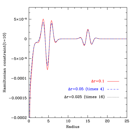
Figure 3: Hamiltonian constraint at $t=10$ for simulations of a pure gauge wave with three different resolutions $\Delta r=0.1$, $\Delta r=0.05$, and $\Delta r=0.025$ rescaled by the factors corresponding to second-order convergence.

The Schwarzschild metric in isotropic coordinates is used as initial data to test the ability of the code to evolve BH spacetimes within the moving puncture approach. The initial data are such that the 3-metric is written as

$$dl^{2}=\psi^{4}(dr^{2}+r^{2}d\Omega^{2}),$$ (41)

where the conformal factor is $\psi=(1+{M}/{2r})$, $M$ being the mass of the BH, which we set as $M=1$. Here $r$ is the isotropic radius. Initially the extrinsic curvature is $K_{ij}=0$.

Figure 4: Time evolution of the maximum value of the radial shift $\beta^{r}$ (upper panel), and of the mass of the AH (lower panel) in the single puncture BH simulation.

We evolve the single stationary puncture initial data with a precollapsed lapse and initially vanishing shift vector. We use the gauge conditions given by Eqs. (20)–(22), with a resolution $\Delta r=0.05$, $\Delta t=0.5\Delta r$ and $N_{r}=30000$ grid points to place the outer boundary sufficiently far way from the puncture so that errors from the boundary do not affect the evolution.

As pointed out by Hannam07 ; Hannam07b , the numerical slices of a Schwarzschild BH spacetime with these gauge conditions reach a stationary state after $t\sim 20$. This is shown in Fig. 4, where the time evolution of the maximum value of the radial shift $\beta^{r}$ is displayed in the upper panel. After an initial phase in which the maximum value of the shift vector grows rapidly, it settles to a value of $\sim 0.15$ and we find almost no drift until the end of the simulation at $t=2500$. In the lower panel of Fig. 4, we show the time evolution of the mass of the apparent horizon (AH), defined as $M_{\rm{AH}}=\sqrt{{\mathcal{A}}/{16\pi}}$, where $\mathcal{A}$ is the area of the AH. We notice that $M_{\rm{AH}}$ is conserved well during the evolution and the error at $t=2500$ is less than $0.2\%$

Figure 5: L2-norm of the Hamiltonian constraint in the single puncture BH simulation. The insets show the L2-norm during the initial phase, and the L2-norm computed outside the AH respectively.

The Hamiltonian constraint violation results are displayed in Fig. 5, which shows the L2-norm of the Hamiltonian constraint as a function of time. Both the initial phase driven by the gauge dynamics (see upper inset in Fig. 5) and the stationary phase are clearly visible. The lower inset in Fig. 5 shows that the L2-norm computed outside the AH is about three orders of magnitude smaller than the L2-norm computed in the whole grid, which is to be expected as the largest spatial violation of the constraint occurs near the puncture (due to the finite differencing of the irregular solution).

V.3 Spherical relativistic stars

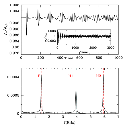
Figure 6: Upper panel shows the time evolution of the normalized central density for an $M=1.4$, $\kappa=100$, $N=1$ polytrope. Power spectrum of the evolution of the central rest-mass density is shown in the lower panel. F, H1 and H2 represent the frequency of the fundamental mode and the first two overtones computed by Font02c .

For our first numerical simulation of the coupling of Einstein equations and the general relativistic hydrodynamic equations, we use the Tolman-Oppenheimer-Volkoff (TOV) solution. We focus on an initial TOV model that has been extensively investigated numerically by Font00c ; Font02c . This model is a relativistic star with polytropic index $N=1$, polytropic constant $\kappa=100$ and central rest-mass density $\rho_{c}=1.28\times 10^{-3}$, so that its gravitational mass is $M=1.4$, its baryon rest-mass $M_{*}=1.5$ and its radius $R=9.59$.

We evolve these initial data with our non-linear code until $t=3000$ ($\sim$17 ms). In the upper panel of Fig. 6 we plot the time evolution of the central rest-mass density for a simulation with $\Delta r=0.025$ and $N_{r}=4000$ until $t=1000$. In the inset we show the same quantity for the whole evolution. We observe that the truncation errors at this resolution are enough to excite small periodic radial oscillations, visible in this plot as periodic variations of the central density. We see that the damping of the periodic oscillations of the central rest-mass density is very small during the whole evolution, which highlights the low numerical viscosity of the implemented scheme.

By computing the Fourier transform of the time evolution of the central rest-mass density we obtain the power spectrum, which is shown with a solid line in the lower panel of Fig. 6, while the dashed vertical lines indicate the fundamental frequency and the first two overtones computed by Font02c . Note that the locations of the frequency peaks for the fundamental mode and the two overtones are in very good agreement, the relative error in the fundamental frequencies being less than 0.1%.

The result of this simulation shows the ability of the scheme to maintain the numerical stability in long-term non-vacuum regular spacetime simulations in spherical coordinates without the need of an additional regularization at the origin.

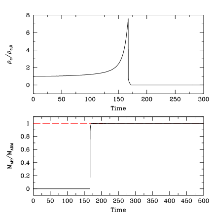
Figure 7: Time evolution of the normalized central density (upper panel) and mass of the AH in units of the ADM mass of the system (lower panel) for the collapse of a marginally stable spherical star to a BH.

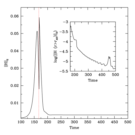
Figure 8: L2-norm of the Hamiltonian constraint in the collapse simulation. The vertical dashed line indicates the time of AH formation. The inset shows the L2-norm computed outside the AH.

V.4 Gravitational collapse of a marginally stable spherical relativistic star

We next test the capability of the code to follow BH formation with the gravitational collapse to a BH of a marginally stable spherical relativistic star. For this test, we consider a $\kappa=100$, $N=1$ polytropic star with central rest-mass density $\rho_{c}=3.15\times 10^{-3}$, so that its gravitational mass is $M=1.64$ and its baryon rest-mass $M_{*}=1.79$. In order to induce the collapse of the star, we initially increase the rest-mass density by 0.5$\%$.

We present numerical results for a simulation of the gravitational collapse of a marginally stable spherical relativistic star performed with resolution of $\Delta r=0.125$. We use the gauge conditions given in Eqs. (20)–(22). We plot in Fig. 7 the time evolution of the normalized central density until $t=300$ (upper panel), and of the mass of the AH in units of the ADM mass of the system until $t=500$ when we stopped the simulation (lower panel). Overall, as the collapse proceeds the star increases its compactness, reflected in the increase of the central density as shown in the upper panel. The most unambiguous signature of the formation of a BH during the simulation is the formation of an AH. Once an AH is found by the AH finder, we monitor the evolution of the AH area, and also of its mass which is plotted, in the lower panel of Fig. 7. This panel shows that approximately at $t\sim 167$, an AH is first found and that the mass of the AH relaxes to the ADM mass of the system. The difference in the ADM mass and the mass of the AH at $t=500$, is about $0.2\%$.

In Fig.8 we plot the L2-norm of the Hamiltonian constraint in the collapse simulation. The vertical dashed line indicates the time of AH formation, and the inset shows the L2-norm computed outside the AH. The largest violation of the constraint occurs during the AH formation, and afterwards the value of the L2-norm settles to $\sim 10^{-3}$. As in the case of a Schwarzschild BH, the L2-norm of the Hamiltonian constraint computed outside the AH is about two orders of magnitude smaller than the L2-norm computed in the whole grid.

Results of this simulation indicate that the numerical scheme to integrate the evolution equations in time can handle accurately the transition between a regular spacetime (that of the star) and a irregular spacetime containing a puncture singularity at $r=0$.

VI Conclusions

In this paper we have presented a numerical code solving the BSSN equations in spherical symmetry and the general relativistic hydrodynamic equations written in flux-conservative form. A key feature of the code is that it uses a second-order PIRK method to integrate the evolution equations in time. This numerical scheme has proved to be crucial and sufficient to obtain the desired stability without the need for a regularization scheme at the origin.

We have performed and discussed a number of tests to assess the accuracy and expected convergence of the code, namely a pure gauge wave, the evolution of a single BH, the evolution of spherical relativistic stars in equilibrium, and the gravitational collapse of a spherical relativistic star leading to the formation of a BH. We remark that, to our knowledge, we have presented the first successful numerical simulations of regular spacetimes (vacuum and non-vacuum) using the covariant BSSN formalism in spherical coordinates without the need for a regularization algorithm at the origin (or without performing a spherical reduction of the equations Garfinkle08 ; Bernuzzi10 ).

In addition, curvilinear coordinate systems facilitate the use of non-uniform radial grids (i.e., logarithmic radial coordinate) to achieve the required high resolution near the origin while still keeping the outer boundaries sufficiently far away. This is particularly useful if one aims to study astrophysical phenomena like the gravitational collapse or the dynamics of accretion disks around BHs. Such approach is simpler, and likely computationally less expensive, than the adaptive mesh refinement techniques used in 3D codes in Cartesian coordinates.

We note that, unlike with the Fully Constrained Formulation FCF in which some of the equations take an elliptic form and where a similar PIRK has been successfully tested, the BSSN formulation is purely hyperbolic, and yet the application of the PIRK method has proved very robust and provided the numerical stability necessary to perform long-term simulations of regular spacetimes in curvilinear coordinates. The work we have presented also paves the way for future comparisons of the performance in curvilinear coordinates between the BSSN and the Fully Constrained Formulation system. Moreover, the application of the PIRK method to the BSSN equations in 3D in such coordinate systems should be rather straight forward, and we aim to investigate this in a future work.

Appendix A Detailed source terms included in the PIRK operators for the evolution equations

The evolution Eqs. (6), (7), (II.1), (II.1), (II.1), (17), (20)-(22), are evolved using a second-order PIRK method, described in Sec. III. In this Appendix the source terms included in the explicit or partially implicit operators are detailed.

Firstly, the hydrodynamic conserved quantities, $a$, $b$, $X$, $\alpha$ and $\beta^{r}$, are evolved explicitly, i.e., all the source terms of the evolution equations of these variables are included in the $L_{1}$ operator of the second-order PIRK method.

Secondly, $A_{a}$ and $K$ are evolved partially implicitly, using updated values of $\alpha$, $a$ and $b$; more specifically, the corresponding $L_{2}$ and $L_{3}$ operators associated to the evolution equations for $A_{a}$ and $K$ are:

$$L_{2(A_{a})} =-\left(\nabla^{r}\nabla_{r}\alpha-\frac{1}{3}\nabla^{2}\alpha\right)+\alpha\left(R^{r}_{r}-\frac{1}{3}R\right),$$ (42)

$$L_{3(A_{a})} =\beta^{r}\partial_{r}A_{a}+\alpha KA_{a}-16\pi\alpha(S_{a}-S_{b}),$$ (43)

$$L_{2(K)} =-\nabla^{2}\alpha,$$ (44)

$$L_{3(K)} =\beta^{r}\partial_{r}K+\alpha(A_{a}^{2}+2A_{b}^{2}+\frac{1}{3}K^{2})$$

$$+4\pi\alpha(E+S_{a}+2S_{b}).$$ (45)

Then, $\hat{\Delta}^{r}$ is evolved partially implicitly, using updated values of $\alpha$, $a$, $b$, $\beta^{r}$, conformal factor, $A_{a}$ and $K$; more specifically, the corresponding $L_{2}$ and $L_{3}$ operators associated to the evolution equation for $\hat{\Delta}^{r}$ are:

$$L_{2(\hat{\Delta}^{r})} =\frac{1}{a}\partial^{2}_{r}\beta^{r}+\frac{2}{b}\partial_{r}\left(\frac{\beta^{r}}{r}\right)+\frac{\sigma}{3a}\partial_{r}(\hat{\nabla}_{m}\beta^{m})$$

$$-\frac{2}{a}(A_{a}\partial_{r}\alpha+\alpha\partial_{r}A_{a})-\frac{4\alpha}{rb}(A_{a}-A_{b})$$

$$+\frac{\xi\alpha}{a}\left[\partial_{r}A_{a}-\frac{2}{3}\partial_{r}K+6A_{a}\partial_{r}\chi\right.$$

$$\left.+(A_{a}-A_{b})\left(\frac{2}{r}+\frac{\partial_{r}b}{b}\right)\right],$$ (46)

$$L_{3(\hat{\Delta}^{r})} =\beta^{r}\partial_{r}\hat{\Delta}^{r}-\hat{\Delta}^{r}\partial_{r}\beta^{r}+\frac{2\sigma}{3}\hat{\Delta}^{r}\hat{\nabla}_{m}\beta^{m}$$

$$+2\alpha A_{a}\hat{\Delta}^{r}-8\pi j_{r}\frac{\xi\alpha}{a}.$$ (47)

Finally, $B^{r}$ is evolved partially implicitly, using updated values of $\hat{\Delta}^{r}$, i.e., $\displaystyle L_{2(B^{r})}=\frac{3}{4}\partial_{t}\hat{\Delta}^{r}$ and $L_{3(B^{r})}=0$.

References

- (1) T. Nakamura, K. Oohara and Y. Kojima, Prog. Theor. Phys. Suppl. 90, 1 (1987).
- (2) M. Shibata and T. Nakamura, Phys. Rev. D 52, 5428 (1995).
- (3) T. W. Baumgarte and S. L. Shapiro, Phys. Rev. D 59, 024007 (1998).
- (4) M. Campanelli, C. O. Lousto, P. Marronetti and Y. Zlochower, Phys. Rev. Lett. 96, 111101 (2006).
- (5) J. G. Baker, J. Centrella, D. I. Choi, M. Koppitz and J. van Meter, Phys. Rev. Lett. 96, 111102 (2006).
- (6) J.D. Brown, Phys. Rev. D 79, 104029 (2009).
- (7) J.M. Bardeen and T. Piran, Phys. Rep. 96, 205 (1983).
- (8) M. W. Choptuik, Phys. Rev. D 44, 3124 (1991).
- (9) O. Rinne and J.M Stewart, Class. Quant. Grav. 22, 1143 (2005).
- (10) M. Alcubierre and J.A. González, Comp. Phys. Comm. 167, 76 (2005).
- (11) M. Ruiz, M. Alcubierre and D. Nuñez, Gen. Rel. Grav. 40, 159 (2007).
- (12) M. Alcubierre and M.D. Mendez, Gen. Rel. Grav. 43, 2769 (2011).
- (13) I. Cordero-Carrión, P. Cerdá-Durán and J.M. Ibáñez, Phys. Rev. D 85, 044023 (2012).
- (14) S. Bonazzola, E. Gourgoulhon, P. Grandclément and J. Novak, Phys. Rev. D 70, 104007 (2004).
- (15) I. Cordero-Carrión. To appear in the proceedings of the ’Numerical Methods for Hyperbolic Equations: Theory and Applications’ conference, Santiago de Compostela (Spain, 2011).
- (16) I. Cordero-Carrión and P. Cerdá-Durán. In preparation.
- (17) F. Banyuls, J. A. Font, J. M. Ibánez, J. M. Martí and J. A. Miralles, Astrophys. J. 476, 221 (1997).
- (18) C. Bona, J. Massó, E. Seidel and J. Stela, Phys. Rev. D 56, 3405 (1997).
- (19) M. Alcubierre, B. Brügmann, P. Diener, M. Koppitz, D. Pollney, E. Seidel and R. Takahashi, Phys. Rev. D 67, 084023 (2003).
- (20) S. Gottlieb and C.-W. Shu, Math. Compt. 67, 73–85 (1998).
- (21) H.-O. Kreiss and J. Oliger, in Methods for the Approximate Solution of the Time Dependent Problems, edited by GARP Publ. Ser. (Geneva, 1973).
- Harten et al. (1983) A. Harten, P.D. Lax and B.& van Leer, SIAM Rev. 25, 35 (1983).
- Einfeldt (1988) B. Einfeldt, SIAM J. Numer. Anal. 25, 294 (1988).
- (24) J. A. Font, T. Goodale, S. Iyer, M. Miller, L. Rezzolla, E. Seidel, N. Stergioulas, W. M. Suen and M. Tobias, Phys. Rev. D 65, 084024 (2002).
- (25) M. Hannam, S. Husa, B. Brügmann, J. A. Gonz lez, U. Sperhake and N. OMurchadha, J. Phys. Conf. Ser. 66, 012047 (2007).
- (26) M. Hannam, S. Husa, D. Pollney, B. Brügmann and N. OMurchadha, Phys. Rev. Lett. 99, 241102 (2007).
- (27) J.A. Font, N. Stergioulas and K.D. Kokkotas, MNRAS 313, 678 (2000).
- (28) D. Garfinkle, C. Gundlach and D. Hilditch, Class. Quant. Grav. 25, 075007 (2008).
- (29) S. Bernuzzi and D. Hilditch, Phys. Rev. D 81, 084003 (2010).