Hyperbolic Relaxation Method for Elliptic Equations

Abstract

We show how the basic idea of parabolic Jacobi relaxation can be modified to obtain a new class of hyperbolic relaxation schemes that are suitable for the solution of elliptic equations. Some of the analytic and numerical properties of hyperbolic relaxation are examined. We describe its implementation as a first order system in a pseudospectral evolution code, demonstrating that certain elliptic equations can be solved within a framework for hyperbolic evolution systems. Applications include various initial data problems in numerical general relativity. In particular we generate initial data for the evolution of a massless scalar field, a single neutron star, and binary neutron star systems.

I Introduction

The solution of elliptic partial differential equations (elliptic PDEs) is an important problem in many areas of physics, including fluid dynamics, quantum mechanics, general relativity, and many more besides. Correspondingly large is the variety of analytic and numerical methods dealing with the solution of elliptic PDEs. The starting point for many methods is a discretization and (if required) a linearization, which for typical problems arising in physics leads to a sparse system of linear equations for a large but finite number of degrees of freedom.

A key role in the solution of linear systems is played by iterative methods, e.g. Saad (2003); Saad and van der Vorst (2000). Among the basic iterative methods are relaxation methods, in particular Gauss-Seidel and Jacobi relaxation methods, and the family of Krylov subspace methods. Closely connected are strategies to accelerate the convergence of such methods, such as preconditioners and multigrid methods.

In this paper we study a modification of the classic Jacobi method, which is motivated by its origin in physical relaxation problems. For concreteness, consider as a minimal example the Laplace equation,

$$\Delta\phi=0,$$ (1)

for a function $\phi(x,y,z)$ on a regular subset of $\mathbb{R}^{3}$ together with appropriate boundary conditions. The Jacobi relaxation scheme can be obtained by introducing a time parameter $t$ and considering instead of (1) the parabolic diffusion equation

$$\partial_{t}\phi=\Delta\phi.$$ (2)

As time approaches infinity, any initial data for $\phi$ “relaxes” to a stationary state, where $\partial_{t}\phi=0$ and hence $\Delta\phi=0$ (1) is satisfied as well. The Jacobi iteration method is obtained by discretizing the diffusion equation (2). In essence, we introduce an “unphysical” time dependence, which is not part of the original problem, and obtain the solution to the time-independent problem by means of a fixed point iteration.

In this paper we investigate a similar strategy, which however relies on a different type of evolution equation. Instead of replacing the elliptic equation (1) by the parabolic equation (2), we consider a hyperbolic wave equation with damping,

$$\partial_{t}^{2}\phi+\partial_{t}\phi=\Delta\phi.$$ (3)

Combining time derivatives as in (3) adds strong diffusion to the pure wave equation while maintaining the hyperbolic character of the PDE. The idea is that deviations from the stationary state satisfying $\Delta\phi=0$ are damped to zero or are propagated away, and furthermore it can be advantageous to perform hyperbolic as opposed to parabolic evolutions.

In the limit of vanishing damping we obtain the wave equation

$$\partial_{t}^{2}\phi=\Delta\phi.$$ (4)

If a stationary state is reached, we again have solved (1). Experimenting with (3) we found that the damping is the main desirable feature, while propagating waves off the grid is far less relevant for the reduction of the residual. Therefore, the proposal is to study (3) for a variety of elliptic operators with strong damping.

Hyperbolic equations containing diffusion or viscosity terms are a well-known topic, e.g. Hsiao and Liu (1992); Nishihara (1997); Wirth (2014), which is relevant to our discussion, see Sec. II.1. The topic revolves around applying relaxation methods to hyperbolic equations, in particular hyperbolic conservation laws with diffusion. Although the type of equations that are considered are similar, our perspective is different. The elliptic equation is for us the fundamental problem, and we add a hyperbolic, damped time-dependence to obtain an iterative scheme for the solution of the elliptic equation. Since there does not seem to be an established name for this idea, we refer to the method as hyperbolic relaxation for elliptic equations (HypRelax), as opposed to parabolic relaxation that is at the heart of the Jacobi method.

With regard to previous literature on hyperbolic relaxation for elliptic equations, some aspects have been explored in Alcubierre et al. (2003) in the context of “gauge drivers” for numerical relativity. In particular, Alcubierre et al. (2003) introduced one of the most used gauge conditions for certain black hole evolutions, the Gamma-driver for the shift vector, which employs a hyperbolic equation related to the elliptic equation for a minimal distortion shift. Also see Balakrishna et al. (1996) on gauge drivers, where however only parabolic relaxation is considered.

The goal of the present paper is to develop hyperbolic relaxation given by the prototype in (3) into a method to solve a general class of second order, non-linear elliptic equations. The basic observation that elliptic equations can be related to the stationary end points of evolutions is well known. However, the challenge is to develop a concrete formulation of a hyperbolic relaxation method that can solve non-trivial problems. The problem of immediate interest to us is defined by the constraint equations of general relativity, which we solve as a system of non-linear elliptic equations to obtain initial data for evolution in numerical relativity. However, the formalism is quite independent of this particular problem.

The main result of this paper is that hyperbolic relaxation can be formulated for non-trivial equations, and numerical experiments for some specific test problems were indeed successful. Specific examples include the Poisson equation, the conformal-thin-sandwich equations, scalar field initial data, and some simple configurations of single and binary neutron stars.

Considering (3), let us collect some basic observations here in order to introduce the main questions we want to address. First of all, we have to address the well-posedness of the hyperbolic PDEs. Given a self-adjoint, elliptic operator, the hyperbolicity of equations of type (3) should be clear. We demonstrate this below for a general class of equations. There exists a rich theoretical background regarding well-posedness and numerical stability for hyperbolic PDEs Gustafsson et al. (1995); Sarbach and Tiglio (2012); Hilditch (2013), which helps to find relaxation schemes that are well suited for numerical applications. However, evolutions of hyperbolic PDEs are not trivial, so we should expect that some elliptic problems are not amenable to hyperbolic relaxation while others are, which is why we include a non-trivial set of test problems below.

Second, in addition to the boundary conditions of the original elliptic equation we have to choose boundary conditions for the hyperbolic equations that are compatible with the asymptotic elliptic problem This choice is not unique, but of great importance to obtain successful evolutions. In particular, we consider maximally dissipative boundary conditions.

Third, assuming feasibility and stability of hyperbolic relaxation, a key question concerns the efficiency of the method. In both parabolic and hyperbolic relaxation methods the time parameter is unrelated to the elliptic equation, i.e. the time evolution is of no interest as long as the stationary state is reached efficiently. This is the basis for different acceleration strategies. For hyperbolic relaxation, there is a finite propagation speed, and in contrast to the diffusion equation it is not clear how to by-pass that speed to accelerate the method.

Beyond the intrinsic interest in a new method, we have to ask whether hyperbolic relaxation, after some significant further development that is beyond the scope of this paper, might become an interesting alternative to the highly developed standard methods.

As it stands, there are pragmatic considerations that can make hyperbolic relaxation methods interesting, in particular when solving elliptic equations as part of a larger project. For example, elliptic PDEs are often solved to provide initial data for evolution systems that are subject to certain constraint equations, e.g. the Maxwell equations or the Einstein equations. However, the main work load is the actual evolution of the data by integrating a hyperbolic PDE. In such a case the hyperbolic relaxation method does not have to compete with optimized standard methods in terms of efficiency as long as solving the elliptic equation is only a small part of the entire work load. On the other hand, a hyperbolic relaxation method may be easy to implement using the existing infrastructure of a numerical evolution code, avoiding the need for and the complications of an external elliptic solver. Using the same infrastructure also has the advantage that interpolation errors can be avoided by using the same grid discretization. Considering our research in numerical relativity, a sophisticated infrastructure for evolutions is indeed available, but we were looking for alternative elliptic solvers. Hence we implemented hyperbolic relaxation in the pseudospectral hyperbolic evolution code bamps Brügmann (2013); Hilditch et al. (2016), which only required minor modifications once the formalism itself was established.

The paper is structured as follows. In Sec. II we derive and motivate the evolution equations on which our relaxation method is based and discuss some of its properties. In Sec. III we give details on the numerical implementation and state the methods used in the bamps code. In Secs. IV and V we apply our hyperbolic relaxation method to some test cases and to the construction of initial data for numerical relativity. We conclude in Sec. VI.

Throughout the paper we use the Einstein summation convention, i.e. we sum over indices that occur once as an upper index and once as a lower index, e.g. $s^{i}t_{i}=\sum_{i}s^{i}t_{i}$. Latin letters $i,j,k,...$ denote coordinate components and they are lowered and raised by an arbitrary metric with positive signature. An index $s$ denotes a contraction with a vector $s_{i}$, in particular $\partial_{s}=s^{i}\partial_{i}=s^{i}\frac{\partial}{\partial x^{i}}$. Greek letter indices $\alpha,\beta,\gamma$ denote components of a field and they are lowered and raised by the Euclidean metric. We also use Latin letters $a,b,c$ to denote the spacetime components in general relativity and which are lowered and raised by the spacetime metric $g_{ab}$.

II The Hyperbolic Relaxation Equations

II.1 Evolution System

In the following we present the principal ideas of the hyperbolic relaxation method and derive the equations that follow for the iteration scheme. In this paper we consider only systems of elliptic equations given in second order form, i.e.

$$(L\psi)_{\alpha}={a(x^{k})}\indices{{}^{i}{}^{j}{}^{\beta}_{\alpha}}\partial_{i}\partial_{j}\psi_{\beta}+F_{\alpha}(x^{k},\psi_{\beta},\partial_{i}\psi_{\beta})=0\,,$$ (5)

where the $\psi_{\alpha}$ are the $N$ unknown solution variables and $F$ is a continuous function of the solution variables, their derivatives and the $D$ coordinates $x^{k}$. We take $a\indices{{}^{i}{}^{j}{}^{\beta}_{\alpha}}$ to be a smooth function of the coordinates and suppress this dependence in the notation. In the following we consider classically elliptic systems Dain (2006) only, i.e. systems with

$$\det(a(x^{k})\indices{{}^{i}{}^{j}{}^{\beta}_{\alpha}}s_{i}s_{j})\neq 0~{}~{}~{}~{}\forall s\in\mathbb{R}^{D}\setminus\{0\}\,,$$ (6)

where the determinant is understood to be taken on the indices $\alpha$ and $\beta$.

Every elliptic system will be accompanied by a set of boundary conditions on the variables $\psi_{\alpha}$ and we discuss their treatment in section II.5. We can reduce the second order elliptic system to first order by introducing the reduction variables $r_{i\alpha}$:

$$0 =a\indices{{}^{i}{}^{j}{}^{\beta}_{\alpha}}\partial_{i}r_{j\beta}+F_{\alpha}(\psi_{\beta},r_{i\beta})\,,$$ (7)

$$0 =\partial_{i}\psi_{\alpha}-r_{i\alpha}\,.$$ (8)

To solve the second order equation (5) one could employ the Jacobi method, which can be motivated by evolving the parabolic partial differential equation:

$$\partial_{t}\psi_{\alpha}=(L\psi)_{\alpha}\,,$$ (9)

where $t$ is some parameter that plays the role of time.

For a classically elliptic system with constant coefficients the Jacobi method can only converge if $a\indices{{}^{j}{}^{i}{}^{\beta}_{\alpha}}$ is positive definite on the whole domain, i.e. there exists an $\epsilon>0$

$$a\indices{{}^{j}{}^{i}{}^{\beta}_{\alpha}}t_{j\beta}t\indices{{}_{i}^{\alpha}}\geq\epsilon t^{i\alpha}t_{i\alpha}~{}~{}~{}~{}\forall t\in\mathbb{R}^{D\times N}\setminus\{0\}\,,$$ (10)

which we assume in the rest of this paper. This condition corresponds to the notion of strong ellipticity, which defines an important subclass of classically elliptic systems Dain (2006). Note that we have the freedom to multiply the elliptic equation with an invertible matrix $d\indices{{}^{\beta}_{\alpha}}$, yielding $(\tilde{L}\psi)_{\alpha}=d\indices{{}^{\beta}_{\alpha}}(L\psi)_{\beta}=0$, which has the same solutions as the original equation. This freedom allows us to transform some systems into a strongly elliptic system, that originally were not.

In analogy to the Jacobi method (9) we evolve $\psi_{\alpha}$ by taking Eq. (7) as the right-hand side, yielding

$$\partial_{t}\psi_{\alpha}=a\indices{{}^{i}{}^{j}{}^{\beta}_{\alpha}}\partial_{i}r_{j\beta}+F_{\alpha}(x^{i},\psi_{\beta},r_{i\beta})$$ (11)

and we proceed similarly with the equations for the reduction variables $r_{i}$:

$$\partial_{t}r_{i\alpha}=b\indices{{}^{j}_{i}{}^{\beta}_{\alpha}}(\partial_{j}\psi_{\beta}-r_{j\beta})\,,$$ (12)

where $b\indices{{}^{j}_{i}{}^{\beta}_{\alpha}}$ is arbitrary under the requirement of positive definiteness, meaning in analogy to Eq. (10)

$$b\indices{{}^{j}_{i}{}^{\beta}_{\alpha}}t_{j\beta}t^{i\alpha}>\epsilon t_{i\alpha}t^{i\alpha}~{}~{}~{}~{}\forall t\in\mathbb{R}^{D\times N}\setminus\{0\}\,.$$ (13)

The system of Eqs. (11) and (12) forms a first order hyperbolic differential equation which we refer to as the the hyperbolic relaxation system. Clearly the reduction constraint Eq. (8) is not enforced at all times and will indeed be violated during the relaxation process, however we are only interested in the steady state, which fulfills the reduction constraint, because Eq. (12) constantly drives the reduction variable $r_{i}$ towards $\partial_{i}\psi$. To see this, let us assume for arguments sake that $\partial_{t}\partial_{i}\psi_{\alpha}=0$. Then the solution for $r_{i\alpha}$ has the form

$$r_{i\alpha}(t)=\sum_{l=1}^{n}e^{-\lambda_{l}t}\sum_{k_{l}=0}^{m_{l}}{x^{k_{l}}h_{k_{l}i\alpha}}+\partial_{i}\psi_{\alpha}\,,$$ (14)

where $h$ is constant and the $\lambda_{l}$ are the $n$ eigenvalues defined by the eigenvalue equation $b\indices{{}^{j}_{i}{}^{\beta}_{\alpha}}t\indices{{}_{l}^{i}{}^{\alpha}}=\lambda_{l}t\indices{{}_{l}^{j}{}^{\beta}}$ and $m_{l}$ depends on the geometric multiplicity of $\lambda_{l}$. From the positive definiteness of $b$ we know that all the eigenvalues have positive real part and it follows immediately that $r_{i\alpha}$ approaches $\partial_{i}\psi_{\alpha}$ exponentially. We emphasize however that in some cases, e.g. if the elliptic system has no solution, $\partial_{i}\psi_{\alpha}$ can grow faster than $r_{i\alpha}$ and thus the reduction constraints cannot be satisfied asymptotically in time.

Assuming that the solution to the elliptic system exists and is unique under the provided boundary conditions, then it is obvious that if the hyperbolic relaxation system reaches a steady state, then we must have the solution to the first order elliptic system Eqs. (7) and (8), and also of the original elliptic equation (5).

The relationship between hyperbolic equations and parabolic diffusion equations has already been investigated in some special cases Hsiao and Liu (1992); Nishihara (1997); Wirth (2014). In particular it can be shown that for large times $t$ the solution of the hyperbolic equation

$$\partial_{t}^{2}\phi+\partial_{t}\phi-\Delta\phi=0$$ (15)

will tend towards the solution of the parabolic PDE

$$\partial_{t}\phi-\Delta\phi=0\,.$$ (16)

The hyperbolic equation can be cast in first order form by introducing the reduction variables $\psi=\partial_{t}\phi+\phi$ and $r_{i}=\partial_{i}\phi$, yielding the system

$$\partial_{t}\phi =\psi-\phi\,,$$ (17)

$$\partial_{t}\psi =\delta^{ij}\partial_{i}r_{j}\,,$$ (18)

$$\partial_{t}r_{i} =\partial_{i}\psi-r_{i}\,.$$ (19)

Clearly the first of these equations is an ordinary differential equation that has no direct counterpart in our hyperbolic relaxation system, however it is directly evident that $\phi$ will tend towards $\psi$ exponentially. Thus it is plausible that for large $t$ the variable $\psi$ of our hyperbolic relaxation system will behave similarly to that of the Jacobi-type relaxation equation (9).

II.2 Residual Evolution

The residuals of the first order system, Eqs. (7),(8), are given by

$$R_{\alpha} =a\indices{{}^{i}{}^{j}{}^{\beta}_{\alpha}}\partial_{i}r_{j\beta}+F_{\alpha}(x^{i},\psi_{\beta},r_{i\beta})\,,$$ (20)

$$R_{i\alpha} =b\indices{{}^{j}_{i}{}^{\beta}_{\alpha}}(\partial_{j}\psi_{\beta}-r_{j\beta})\,.$$ (21)

A simple calculation shows that the residuals will evolve according to

$$\partial_{t}R_{\alpha} =a\indices{{}^{i}{}^{j}{}^{\beta}_{\alpha}}\partial_{i}R_{j\beta}+\frac{\partial F_{\alpha}}{\partial\psi_{\beta}}R_{\beta}+\frac{\partial F_{\alpha}}{\partial r_{i\beta}}R_{i\beta}\,,$$ (22)

$$\partial_{t}R_{i\alpha} =b\indices{{}^{j}_{i}{}^{\beta}_{\alpha}}(\partial_{j}R_{\beta}-R_{j\beta})\,.$$ (23)

For a working relaxation scheme, we want the residual evolution system to be stable, i.e. the first order residuals should converge to zero for $t\rightarrow\infty$, for residuals that are sufficiently close to zero. Systems of this type and stability conditions are discussed in detail in Kreiss et al. (1998) and Kreiss and Lorenz (1998). It is not possible for us to give general results on the stability of the hyperbolic relaxation scheme, as the multitude of possible systems is too large to be covered in a closed form, especially for elliptic systems with more than one variable. A stability analysis must therefore be done individually for the concrete problem.

II.3 Mode Analysis

To shed some light on the behavior of solutions to the hyperbolic relaxation equation (15), we perform a simple mode analysis, ignoring the issue of boundary conditions. Introduce the plane-wave ansatz

$$\phi_{pw}(t,x)=e^{i(kx-\omega t)},$$ (24)

where $k$ and $\omega$ are constants. The wavenumber $k$ is a real number related to the wave length, $k=2\pi/\lambda$, while $\omega$ may be a complex number. Inserted into the hyperbolic relaxation equation (15), we obtain

$$\omega^{2}+i\omega =k^{2},$$ (25)

$$\omega_{\pm}(k) =-\frac{1}{2}(i\pm\sqrt{4k^{2}-1}).$$ (26)

Recall that for the wave equation $\omega_{\pm}(k)=\pm k$, while for the heat equation $\omega(k)=-ik^{2}$. For hyperbolic relaxation, there is a further case distinction for the sign under the square root $\sqrt{4k^{2}-1}$.

For sufficiently large wavenumber,

$$\phi_{pw}=e^{-\frac{1}{2}t}e^{i(kx\pm\frac{1}{2}\sqrt{4k^{2}-1}\,t)},\quad k\geq\frac{1}{2},$$ (27)

which is a damped wave with phase velocity $v(k)=\sqrt{1-\frac{1}{4k^{2}}}$. The damping is independent of $k$ (as opposed to the heat equation with $e^{-k^{2}t}$). The phase velocity approaches $v=1$ for large $k$, but for $k$ approaching the critical value $\frac{1}{2}$ from above the phase velocity tends towards $v=0$.

For sufficiently small wavenumber,

$$\phi_{pw}=e^{-\frac{1}{2}(1\pm\sqrt{1-4k^{2}})t}e^{ikx},\quad 0\leq k\leq\frac{1}{2},$$ (28)

which is a non-moving wave profile $e^{ikx}$ times a $k$-dependent damping factor. For $k=\frac{1}{2}$, the damping is $e^{-\frac{1}{2}t}$, while for $k$ equal to zero there are two cases, $-\frac{1}{2}(1\pm\sqrt{1-4k^{2}})t=0$ or $-t$. For small $k$, the worse (more weakly) damped case is $-\frac{1}{2}(1\pm\sqrt{1-4k^{2}})t\approx-k^{2}t$, which is the same damping as for the basic heat equation.

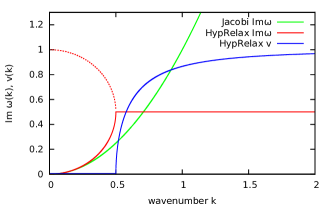
Figure 1: Damping and propagation speed of basic hyperbolic relaxation compared to parabolic relaxation. There is a transition at $k_{crit}=\frac{1}{2}$, which can be moved to lower values by introducing additional parameters. The overall damping is determined by the slowest damping rate.

Summarizing, the plane-wave mode analysis suggests that solutions to the hyperbolic relaxation equation exhibit a mixture of relaxation and wave propagation phenomena, see Fig. 1. For wave numbers larger than a critical value, $k\geq k_{crit}$ with $k_{crit}=\frac{1}{2}$, there is wave propagation with simultaneous damping. Noteworthy is that the damping is independent of $k$, $e^{-\frac{1}{2}t}$. This is a promising feature compared to parabolic relaxation with $e^{-k^{2}t}$ for intermediate values of $k$. For large values of $k$ parabolic relaxation has much stronger damping, but the overall convergence rate is dominated by small $k$. For hyperbolic relaxation, there is no wave propagation for $k\leq k_{crit}$, but the damping persists. Interestingly, the damping factor asymptotes towards $e^{-k^{2}t}$ for $k\rightarrow 0$, and is never worse than parabolic relaxation for small $k$.

The existence of a transition at a specific length scale $\lambda_{crit}=\frac{2\pi}{k_{crit}}=4\pi$ signals that our choice of hyperbolic relaxation equation has fixed a scale. Let us generalize (15) to

$$\epsilon\partial_{t}^{2}\phi+\eta\partial_{t}\phi=\Delta\phi,$$ (29)

where $\epsilon$ and $\eta$ are real, non-negative constants. A third constant in front of $\Delta\phi$, the velocity squared $v^{2}$ in the basic wave equation, has been rescaled to one without loss of generality. With $\epsilon=\eta=1$ as in (15) we fix the unit of time to be dimensionless (unity since $[T^{2}]=[T]$). If we mimic (11) and (12) by

$$\partial_{t}\psi=\partial_{j}r^{j},\quad\partial_{t}r_{i}=b(\partial_{i}\psi-r_{i}),$$ (30)

with a real constant $b$, then we obtain (29) with $\epsilon=1/b$, $\eta=1$, and

$$\omega_{\pm}(k)=-\frac{1}{2}(ib\pm\sqrt{(4k^{2}-b)b}).$$ (31)

Alternatively, we can take our motivation from the gauge driver construction Alcubierre et al. (2003) and set $\epsilon=1$, $\eta$ an arbitrary non-negative constant, and obtain

$$\omega_{\pm}(k)=-\frac{1}{2}(i\eta\pm\sqrt{4k^{2}-\eta^{2}}).$$ (32)

We also considered $\epsilon=\eta^{2}$ and arbitrary $\eta$ for uniform scaling of time.

The bottom line is that the coefficients in (29) allow us to adjust the size of the critical length scale. For example, for $\epsilon=1$ and $\eta$ arbitrary the critical parameters change to $k_{crit}=\frac{\eta}{2}$, while for $\epsilon=1/b$, $\eta=1$ we find $k_{crit}=\frac{\sqrt{b}}{2}$. The damping for large $k$ becomes $e^{-\frac{\eta}{2}}$ and $e^{-\frac{b}{2}}$, respectively.

To avoid small $k$ that drop below (or too far below) $k_{crit}$, we can adjust $b$ or $\eta$ such that the length scale of $k$ corresponds to the physical size $L$ of the domain, say $\lambda_{crit}=2L$. This will slow down the convergence for large $k$, but will also avoid the severe slow down when the damping approaches that of parabolic relaxation.

II.4 Hyperbolicity Analysis

In this section we introduce a notation for inverse tensors. These have to be understood as the inverse of matrices with respect to the field indices. For example the inverse of the tensor $c\indices{{}^{\beta}_{\alpha}}$ is $(c^{-1})\indices{{}^{\alpha}_{\gamma}}$ and we have

$$c\indices{{}^{\beta}_{\alpha}}(c^{-1})\indices{{}^{\alpha}_{\gamma}}=\delta^{\beta}_{\gamma}\,.$$ (33)

For the hyperbolicity analysis we start with writing the hyperbolic relaxation system in matrix form

$$\partial_{t}{\bf u}={\bf P}^{k}\partial_{k}{\bf u}+h(x^{i},{\bf u})$$ (34)

with

$${\bf P}^{k}=\begin{pmatrix}0&a\indices{{}^{k}{}^{i}{}^{\beta}_{\alpha}}\\ b\indices{{}^{k}_{i}{}^{\beta}_{\alpha}}&0\end{pmatrix}\,,~{}~{}~{}~{}~{}~{}{\bf u}=\begin{pmatrix}\psi_{\alpha}\\ r_{i\alpha}\end{pmatrix}\,.$$ (35)

The principal symbol of this system is then given by

$${\bf P}^{s}={\bf P}^{k}s_{k}=\begin{pmatrix}0&a\indices{{}^{s}{}^{i}{}^{\beta}_{\alpha}}\\ b\indices{{}^{s}_{i}{}^{\beta}_{\alpha}}&0\end{pmatrix}\,,$$ (36)

where $s_{i}$ is an arbitrary unit vector, $s^{i}s_{i}=1$. Suppose $c\indices{{}^{\beta}_{\alpha}}=a\indices{{}^{s}{}^{i}{}^{\epsilon}_{\alpha}}b\indices{{}^{s}_{i}{}^{\beta}_{\epsilon}}$ has a complete set of eigenvectors $w\indices{{}_{\gamma}^{\alpha}}$ with $c\indices{{}^{\beta}_{\alpha}}w\indices{{}_{\gamma}^{\alpha}}=\sigma^{\alpha}_{\gamma}w\indices{{}_{\alpha}^{\beta}}$, where $\sigma^{\alpha}_{\gamma}$ is diagonal. If furthermore all the eigenvalues, i.e. the diagonal elements of $\sigma^{\alpha}_{\gamma}$, are positive then $P^{s}$ has the following left eigenvectors

$${\bf v}^{0}_{j\gamma} =\left(0,\delta^{\alpha}_{\gamma}\delta^{i}_{j}-b\indices{{}^{s}_{j}{}^{\epsilon}_{\gamma}}({b\indices{{}^{s}_{s}}}^{-1})\indices{{}^{\alpha}_{\epsilon}}s^{i}\right)\,,$$ (37)

$${\bf v}^{\pm}_{\gamma} =\left(w\indices{{}_{\gamma}^{\alpha}},\pm(\rho^{-1})^{\delta}_{\gamma}w\indices{{}_{\delta}^{\epsilon}}a\indices{{}^{s}{}^{i}{}^{\alpha}_{\epsilon}}\right)\,,$$ (38)

where $\rho^{\beta}_{\gamma}$ is the root of $\sigma^{\beta}_{\gamma}$, i.e. it is a positive diagonal tensor with $\rho^{\alpha}_{\gamma}\rho^{\beta}_{\alpha}=\sigma^{\beta}_{\gamma}$. Note that of the eigenvectors ${\bf v}^{0}_{j\gamma}$ only $(D-1)N$ are linearly independent, while the ${\bf v}^{\pm}_{\gamma}$ are $2N$ independent vectors. If there exists a constant $K$, independent of $s^{i}$, such that $\|{\bf V}\|_{2}+\|{\bf V}^{-1}\|_{2}<K$, where ${\bf V}$ is an, in general $s^{i}$-dependent, square matrix constructed from a linearly independent set of the eigenvectors ${\bf v}$, then the system is strongly hyperbolic Gustafsson et al. (1995); Hilditch (2013); Sarbach and Tiglio (2012). The characteristic variables $\hat{u}$ and their characteristic speeds $\lambda$ are thus

$$\hat{u}^{0}_{j\gamma} =r_{j\gamma}-b\indices{{}^{s}_{j}{}^{\epsilon}_{\gamma}}({b\indices{{}^{s}_{s}}}^{-1})\indices{{}^{\alpha}_{\epsilon}}s^{i}r_{i\alpha}\,,~{}~{}~{}~{}~{}~{}~{}~{}\lambda^{0}_{i\gamma}=0\,,$$ (39)

$$\hat{u}^{\pm}_{\gamma} =w\indices{{}_{\gamma}^{\alpha}}\psi_{\alpha}\pm(\rho^{-1})^{\delta}_{\gamma}w\indices{{}_{\delta}^{\epsilon}}a\indices{{}^{s}{}^{i}{}^{\alpha}_{\epsilon}}r_{i\alpha}\,,~{}~{}~{}\lambda_{\gamma}^{\pm}=\pm\rho^{\alpha}_{\gamma}e_{\alpha}\,,$$ (40)

where $e_{\alpha}$ denote the Cartesian basis vectors. Note that of the characteristic variables $\hat{u}^{0}_{j\gamma}$ only $(D-1)N$ are linearly independent, while the $\hat{u}^{\pm}_{\gamma}$ are $2N$ independent vectors. From this we can recover the evolved variables in terms of the characteristics:

$$\psi_{\alpha} =\frac{1}{2}(w^{-1})\indices{{}_{\alpha}^{\gamma}}(\hat{u}^{+}_{\gamma}+\hat{u}^{-}_{\gamma})\,,$$ (41)

$$r_{i\alpha} =\hat{u}^{0}_{i\alpha}+b\indices{{}^{s}_{i}{}^{\epsilon}_{\alpha}}(c^{-1})\indices{{}^{\beta}_{\epsilon}}$$

$$\qquad\qquad\cdot\left((w^{-1})\indices{{}_{\beta}^{\delta}}\rho^{\gamma}_{\delta}\frac{\hat{u}^{+}_{\gamma}-\hat{u}^{-}_{\gamma}}{2}-a\indices{{}^{s}{}^{j}{}^{\gamma}_{\beta}}\hat{u}^{0}_{j\gamma}\right)\,.$$ (42)

We can use the freedom in the choice of $b\indices{{}^{j}_{i}{}^{\beta}_{\alpha}}$ to impose certain properties on the hyperbolic relaxation system. In the following we briefly discuss three interesting choices, that fulfill the restrictions we have set for $b$.

1. $b$ is the identity. A very easy and natural choice is $b\indices{{}^{j}_{i}{}^{\beta}_{\alpha}}=\delta^{j}_{i}\delta^{\beta}_{\alpha}$. With this choice we have $c\indices{{}^{\beta}_{\alpha}}=a\indices{{}^{s}{}^{s}{}^{\beta}_{\alpha}}$, which has only eigenvalues with positive real part due to (10). The imaginary part however can be non-vanishing. If however $a\indices{{}^{s}{}^{s}{}^{\alpha}_{\gamma}}=a\indices{{}^{s}{}^{s}_{\gamma}{}^{\alpha}}$, then $c$ is guaranteed to have a complete set of eigenvectors with purely real eigenvalues and thus system is strongly hyperbolic. If we have $a\indices{{}^{i}{}^{j}{}^{\alpha}_{\gamma}}=a\indices{{}^{i}{}^{j}_{\gamma}{}^{\alpha}}$, then the system is even symmetric hyperbolic with symmetrizer:

$${\bf H}=\begin{pmatrix}\delta^{\alpha}_{\gamma}&0\\ 0&a\indices{{}^{i}{}^{j}{}^{\alpha}_{\gamma}}\delta_{jl}\end{pmatrix}\,.$$ (43)

2. $b$ is the transpose of $a$. We can also make the system trivially symmetric hyperbolic by choosing $b\indices{{}^{j}_{i}{}^{\beta}_{\alpha}}=a\indices{{}^{j}_{i}{}_{\alpha}^{\beta}}$. The principal symbol of this system is symmetric and thus the system is symmetric hyperbolic.

3. $b$ is the inverse of $a$. We can choose $b$ to be the inverse of $a$ in the sense that $b$ fulfills $a\indices{{}_{k}^{i}{}^{\alpha}_{\gamma}}b\indices{{}^{j}_{i}{}^{\beta}_{\alpha}}=\delta_{k}^{j}\delta^{\beta}_{\gamma}$. This choice is particularly interesting because we then have $c\indices{{}^{\beta}_{\alpha}}=\delta^{\beta}_{\alpha}$ and thus all the non-zero characteristic speeds have values $\pm 1$. Furthermore the eigenvectors of $c$ become trivial: $w\indices{{}_{\gamma}^{\alpha}}=\delta^{\alpha}_{\gamma}$. A symmetrizer for this system is

$${\bf H}=\begin{pmatrix}\delta^{\alpha}_{\gamma}&0\\ 0&a\indices{{}_{m}^{i}{}^{\alpha}_{\omega}}a\indices{{}^{m}_{l}{}_{\gamma}^{\omega}}\end{pmatrix}\,.$$ (44)

Since all traveling characteristic variables have the same speeds, we consider this the best choice for $b\indices{{}^{j}_{i}{}^{\beta}_{\alpha}}$. A straightforward generalization of this choice allows $b\indices{{}^{j}_{i}{}^{\beta}_{\alpha}}$ to be scaled by a constant factor, which will also uniformly scale the characteristic speeds.

II.5 Boundary Conditions

The basic idea to impose boundary conditions in our method is to modify the right hand side of the hyperbolic relaxation system. The outward pointing unit normal covector $s_{i}$ to the boundary surface is naturally defined by taking the gradient of a scalar field which is increasing across, but constant in the boundary, and then normalizing this gradient to unit magnitude using our arbitrary but fixed metric. This metric is subsequently used to raise the index and form the outward pointing vector $s^{i}$. We restrict our attention to strongly hyperbolic systems, for which a regular ($s^{i}$-dependent) similarity transformation matrix ${\bf T}_{s}$ exists which transforms between our evolved variables ${\bf u}$ and a linearly independent set of the characteristic variables ${\bf\hat{u}}$ given in Eq. (39) and (40)

$${\bf u}={\bf T}_{s}{\bf\hat{u}}\,.$$ (45)

We can then decompose our evolution equations (34) as

$$\partial_{t}{\bf u}={\bf P}^{s}\partial_{s}{\bf u}+{\bf P}^{k}q_{k}^{i}\partial_{i}{\bf u}+h(x^{i},{\bf u})\,,$$ (46)

where $q_{k}^{i}=\delta_{k}^{i}-s_{k}s^{i}$ is the projector onto the boundary surface. We now multiply by ${\bf T}_{s}^{-1}$ and obtain

$${\rm d}_{t}{\bf\hat{u}}= {\bf T}_{s}^{-1}{\bf P}^{s}\partial_{s}{\bf u}+{\bf T}_{s}^{-1}({\bf P}^{k}q_{k}^{i}\partial_{i}{\bf u}+h(x^{i},{\bf u}))$$ (47)

$$= {\bf T}_{s}^{-1}{\bf P}^{s}T_{s}{\bf T}_{s}^{-1}\partial_{s}{\bf u}+T_{s}^{-1}({\bf P}^{k}q_{k}^{i}\partial_{i}{\bf u}+h(x^{i},{\bf u}))$$ (48)

$$= {\bf\Lambda}^{s}{\rm d}_{s}\hat{\bf u}+{\bf T}_{s}^{-1}({\bf P}^{k}q_{k}^{i}\partial_{i}{\bf u}+h(x^{i},{\bf u}))\,.$$ (49)

Here the straight derivative symbol ${\rm d}$ denotes that the transformation matrix stands outside of the derivative, i.e. ${\rm d}_{i}\hat{\bf u}\equiv{\bf T}_{s}^{-1}\partial_{i}{\bf u}$, and ${\bf\Lambda}^{s}$ is a diagonal matrix containing the characteristic speeds. We can now impose boundary conditions on the incoming variables, i.e. those with positive characteristic speeds, by modifying their right hand sides. After the right hand sides have been modified we transform the system back by multiplying with ${\bf T}_{s}$.

II.5.1 Penalty Method

In the penalty method Hesthaven (2000); Hesthaven et al. (2007); Taylor et al. (2010) the boundary conditions are weakly imposed by modifying the right hand sides of the incoming characteristic variables $\hat{u}^{+}_{\gamma}$ in the following way

$${\rm d}_{t}\hat{u}^{+}_{\gamma}\hat{=}D_{t}\hat{u}^{+}_{\gamma}+p(\hat{u}^{+\rm BC}_{\gamma}-\hat{u}^{+}_{\gamma})\,,$$ (50)

where $p$ is the penalty parameter, $u^{+\rm BC}_{\gamma}$ is some given boundary data that we want $\hat{u}^{+}_{\gamma}$ to approach, $D_{t}\hat{u}^{+}_{\gamma}$ is the unmodified right hand side and $\hat{=}$ denotes equality at the boundary. The penalty parameter can not be chosen arbitrarily and we refer the reader to Hilditch et al. (2016) for a detailed derivation of the penalty parameters used in bamps.

II.5.2 Maximally Dissipative Boundary Conditions

Maximally dissipative boundary conditions Gustafsson et al. (1995); Gundlach and Martín-García (2006); Sarbach and Tiglio (2012); Hilditch (2013) will allow us to set boundary conditions of the form

$$s^{i}\partial_{i}\psi_{\alpha}|_{\partial\Omega}=\phi_{\alpha}(\psi_{\beta},\partial_{i}\psi_{\beta},q^{i}_{j}\partial_{i}\partial_{k}\psi_{\beta})\,,$$ (51)

where $\phi$ is a function that is allowed to depend on the coordinates $x^{i}$, the fields $\psi_{\alpha}$, their derivatives and the transverse projections ($q^{i}_{j}=\delta^{i}_{j}-s^{i}s_{j}$) of their second derivatives. For brevity we suppress dependence on all the arguments in the following.

Maximally dissipative boundary conditions are imposed by requiring

$$(\rho^{-1})^{\beta}_{\gamma}w\indices{{}_{\beta}^{\alpha}}\partial_{t}\psi_{\alpha}+w\indices{{}_{\gamma}^{\alpha}}\partial_{s}\psi_{\alpha}=w\indices{{}_{\gamma}^{\alpha}}\phi_{\alpha}\,.$$ (52)

This boundary condition is actually be different from Eq. (51) during the relaxation process. However, again we are only interested in the steady state at the end of the evolution, where we have $\partial_{t}\psi_{\alpha}=0$ and thus the correct boundary condition will be imposed. For numerical stability the functions $\phi_{\alpha}$ must not depend on normal derivatives of the evolved variables. Therefore in (51) in the arguments of $\phi_{\alpha}$ we have to make the replacements $\partial_{i}\psi_{\beta}\rightarrow r_{i\beta}$ and $q^{i}_{j}\partial_{i}\partial_{k}\psi_{\beta}\rightarrow q^{i}_{j}\partial_{i}r_{k\beta}$. For the normal derivatives of the incoming characteristic we obtain the relation

$${\mathrm{d}}_{s}\hat{u}^{+}_{\gamma} =w\indices{{}_{\gamma}^{\alpha}}\partial_{s}\psi_{\alpha}+(\rho^{-1})^{\delta}_{\gamma}w\indices{{}_{\delta}^{\epsilon}}a\indices{{}^{s}{}^{i}{}^{\alpha}_{\epsilon}}\partial_{s}r_{i\alpha}$$ (53)

$$=w\indices{{}_{\gamma}^{\alpha}}\phi_{\alpha}-(\rho^{-1})^{\delta}_{\gamma}w\indices{{}_{\delta}^{\alpha}}\left(\partial_{t}\psi_{\alpha}-a\indices{{}^{s}{}^{j}{}^{\epsilon}_{\alpha}}\partial_{s}r_{j\epsilon}\right)\,,$$ (54)

where in the actual implementation $\partial_{t}\psi_{\alpha}$ is to be replaced by Eq. (11). This equation is now used to impose the boundary condition by replacing the ${\mathrm{d}}_{s}\hat{u}^{+}_{\gamma}$terms in Eq. (47), yielding the modified right hand side

$${\mathrm{d}}_{t}\hat{u}^{+}_{\gamma}\hat{=} D_{t}\hat{u}^{+}_{\gamma}$$

$$-\rho^{\beta}_{\gamma}(w\indices{{}_{\beta}^{\alpha}}\partial_{s}\psi_{\alpha}+(\rho^{-1})^{\delta}_{\beta}w\indices{{}_{\delta}^{\alpha}}\partial_{t}\psi_{\alpha}-w\indices{{}_{\beta}^{\alpha}}\phi_{\alpha})\,.$$ (55)

With the general expression at hand, we now discuss the implementation of typical boundary conditions.

1. Dirichlet conditions. Dirichlet conditions are of the form $\psi_{\alpha}|_{\partial\Omega}=g_{\alpha}$, where the $g_{\alpha}$ are some function defined on the domain boundary $\partial\Omega$. To implement such a boundary condition $\phi_{\alpha}$ has to take the form

$$\phi_{\alpha}=s^{i}r_{i\alpha}+e\indices{{}^{\beta}_{\alpha}}(g_{\beta}-\psi_{\beta})\,,$$ (56)

where $e$ is positive definite, i.e. $e\indices{{}^{\beta}_{\alpha}}t_{\beta}t^{\alpha}>0$. In the steady state we have $\partial_{i}\psi_{\alpha}=r_{i\alpha}$ and thus Eq. (52) becomes $0=e\indices{{}^{\beta}_{\alpha}}(g_{\beta}-\psi_{\beta})$, which is only fulfilled for the requested boundary condition. The positive definiteness of $e$ is important to guarantee stability at the boundary. Suppose we have $\partial_{i}\psi_{\alpha}=r_{i\alpha}$ fixed, then Eq. (52) has the form

$$(\rho^{-1})^{\beta}_{\gamma}w\indices{{}_{\beta}^{\alpha}}\partial_{t}\psi_{\alpha}=w\indices{{}_{\gamma}^{\alpha}}e\indices{{}^{\beta}_{\alpha}}(g_{\beta}-\psi_{\beta})\,,$$ (57)

which would have solutions not asymptoting to $g_{\alpha}$ if $e$ was not positive definite. Besides positive definiteness there are no further restrictions apparent on $e$ and therefore, it can be chosen to be the identity $e\indices{{}^{\beta}_{\alpha}}=\delta^{\beta}_{\alpha}$, which we use in our applications.

2. Neumann conditions. Neumann boundary conditions are of the form $s^{i}\partial_{i}\psi_{\alpha}|_{\partial\Omega}=g_{\alpha}$. Their implementation in our method is straightforward; one just has to take $\phi_{\alpha}=g_{\alpha}$.

3. Robin conditions. Robin boundary conditions are mixture of Dirichlet and Neumann boundary conditions and can be written as $s^{i}\partial_{i}\psi_{\alpha}|_{\partial\Omega}=g_{\alpha}+f^{\beta}_{\alpha}\psi_{\beta}$, where the $f^{\beta}_{\alpha}$ are functions defined on the domain boundary. Their implementation is also straight forward choosing $\phi_{\alpha}=g_{\alpha}+f^{\beta}_{\alpha}\psi_{\beta}$.

III Numerical Setup

III.1 Grid Setup

We employ the pseudospectral hyperbolic evolution code bamps and refer the reader to Hilditch et al. (2016), where the grid setup is explained in detail. Here we only give a short summary of the basic grid setup and numerical method. Our grid consists of different coordinate patches, a cube patch in the center, transition shell patches and outer shell patches. On each patch we have a mapping between local Cartesian coordinates to global Cartesian coordinates, where on shell patches we employ the “cubed sphere” construction Ronchi et al. (1996). The patches themselves can consist of smaller subpatches, which are the smallest units we use for our parallelization scheme. On each subpatch we approximate the fields by a Chebyshev pseudospectral method, i.e. the subpatches are discretized in every direction by the Gauss-Lobatto collocation points. It is then possible to reconstruct the Chebyshev coefficients from the fields values at the collocation points.

The bamps code is adapted to evolutions in three dimensions. For axisymmetric and spherically symmetric problems we use the cartoon method to reduce the computational domain to two or one dimensions respectively Hilditch et al. (2016).

III.2 Integration Method

The time integration for relaxation methods does not require a high order of error convergence, since we are only interested in the steady state at the end of the evolution. More important are the efficiency and stability of the integration algorithm. For the time integration we use the method of lines. It is known that for linear hyperbolic equations the simple forward Euler-method and also explicit second-order Runge-Kutta methods are unstable Gustafsson et al. (1995) and thus are not suited for the integration of the hyperbolic relaxation equations.

In the applications presented in this paper we employ the popular fourth-order Runge-Kutta scheme (RK4), which is stable for hyperbolic equations. This method needs four evaluations of the right-hand side per time step, which appears to be not very efficient. After all, we do not need a very accurate integrator, since we are only interested in approaching the stationary state. Therefore it is worthwhile to investigate other classes of integrators, e.g. multistep methods like the third- or fourth-order Adams schemes Boyd (2001), which effectively only require one or two evaluations per time step and are usually also stable for hyperbolic PDEs. Some simple experiments with the Poisson equation indicated, however, that RK4 is more efficient than RK3 or a fourth order Adams scheme since RK4 allows comparatively large time steps.

Contrary to what is described in Hilditch et al. (2016), we neither use nor need filtering to assure stability in the hyperbolic relaxation method, since the system usually tends towards a stable static or stationary solution automatically.

In our code we have two types of boundaries. On the one hand we have boundaries between different subpatches, and on the other hand the boundaries of our computational domain, in particular the outer boundaries. To treat boundaries between subpatches we employ the penalty method described in Sec. II.5.1 setting the boundary data to be the outgoing characteristic of the neighboring subpatch.

Treating the outer boundary with this method we have to provide a function $g_{\gamma}$ equaling $u^{+\rm BC}_{\gamma}$ at the boundary, i.e.

$$\hat{u}^{+\rm BC}_{\gamma}=w\indices{{}_{\gamma}^{\alpha}}\psi_{\alpha}+(\rho^{-1})^{\delta}_{\gamma}w\indices{{}_{\delta}^{\epsilon}}a\indices{{}^{s}{}^{i}{}^{\alpha}_{\epsilon}}r_{i\alpha}=g_{\gamma}\,.$$ (58)

Such a boundary condition however is very unusual in practice for elliptic equations and thus the penalty method is not suited for the treatment of our outer boundaries. Instead we only use the maximally dissipative boundary conditions described in Sec. II.5.2.

III.3 Initial Guesses

To start the hyperbolic relaxation one has to provide an initial guess to the solution. A suitable initial guess will always depend on the specific form of the problem, in particular it should be chosen such that in the course of the relaxation the variables do not have to cross any points where the equations (e.g. terms in the non-principal part) become singular. In our tests we found the solver to be particularly well behaved when starting with a guess that is stationary in the interior, but not at the boundary. The whole solution then starts to relax from the boundary to the inside. For example in our applications to numerical relativity initial data, taking the flat metric everywhere lead to stable relaxations, which demonstrates a remarkably high robustness that can be achieved by the method. For the reduction variables we simply take the numerical derivative of the initial guess, i.e. ${}^{(\rm ini)}r_{i\alpha}=\partial_{i}{{}^{(\rm ini)}\psi_{\alpha}}$

III.4 Refinement Strategy

To speed up the relaxation process we employ a simple scheme of successive refinement. It can be assumed that the right-hand side of the solution variables $\partial_{t}\psi_{\alpha}$, Eq. (11), is a good approximation to the residual of the elliptic equation $(L\psi)_{\alpha}$, Eq. (5). This however is only true until a discretization limit is reached below which the norm of the residual is no longer decreasing. The norm of the $\partial_{t}\psi_{\alpha}$ will typically continue decreasing until machine precision is reached. This makes it possible to construct an indicator signaling when the discretization limit is reached and thus relaxation should be continued on a higher resolution grid. In particular we choose the following criterion,

$$\int\sum_{\alpha=1}^{N}|\partial_{t}\psi_{\alpha}|dV<c\int\sum_{\alpha=1}^{N}|(L\psi)_{\alpha}|dV\,,$$ (59)

where $c$ is some constant smaller than one. For our applications we found $c=0.1$ to be a choice working reasonably well. We note however that depending on the specific problem also smaller values might be beneficial. Additionally we increase the resolution when the error of the elliptic equation reaches machine precision, i.e. when the norm of $(L\psi)_{\alpha}$ is smaller than $10^{-13}$ times the number of grid points.

We start with relaxing the system on the coarsest grid and check every 1000 relaxation steps whether to proceed relaxation on a finer grid based on whether one of the two criteria mentioned above is fulfilled. The final resolution can be determined by an error bound on the residual of the elliptic equation, or by some predetermined resolution, which may be required for the evolution of the data. For the refinement we increase the resolution on every subpatch by two collocation points in every direction, which is equivalent to adding two Chebyshev modes in every direction. We interpolate the coarse steady state solution to the new subpatches and repeat the procedure until we arrive at the desired resolution. We also find it advisable to use the interpolated values for the reduction variables instead of taking the numerical derivative of the solution variables, since the latter introduces new errors, which costs some extra effort to damp.

IV Application to Test Cases

IV.1 Poisson Equation – Finite Differencing

To provide a reference point independent of the specific pseudospectral methods of bamps, we first discuss a minimal implementation using a finite difference method to solve the Poisson equation. We consider the hyperbolic relaxation equation

$$\partial_{t}^{2}\phi+\eta\partial_{t}\phi=\Delta\phi-\rho,$$ (60)

which we implement as a first order in time, second order in space system,

$$\partial_{t}\phi =\pi-\eta\phi,$$ (61)

$$\partial_{t}\pi =\Delta\phi-\rho.$$ (62)

We consider the fully first order version of this system in Sec. IV.2. At the boundaries we use asymptotic Dirichlet conditions analogous to (56), $\partial_{t}\phi=g-\phi$ and $\partial_{t}\pi=g-\pi$.

We choose centered, second order accurate finite differences in space, and the default time integrator is the classic fourth-order Runge-Kutta method. The numerical domain is an equidistant grid of points in $[-\frac{L}{2},\frac{L}{2}]^{d}$, dimension $d=1$, $2$, or $3$, with Cartesian coordinates. There are $N$ points in each of up to three directions with a total of $V=N^{d}$ points.

Let us discuss some results for vanishing source term, $\rho=0$, and vanishing Dirichlet boundary, $g=0$, where the method has to reduce an initial guess of $\phi=1/(1+x_{j}x^{j})$ and $\pi=0$ at $t=0$ to the asymptotic, late-time value $\phi=\pi=0$.

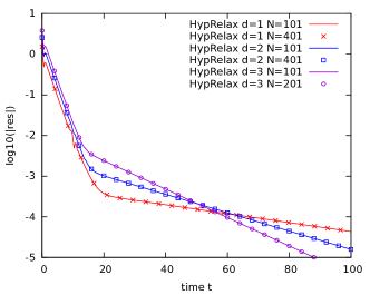
Figure 2: Poisson equation, FD method. Convergence of the residual with time for one, two, and three dimensions. Shown is a solid line for $N=101$ and markers for a higher resolution given by $N=201$ or $401$ points. On the scale of the plot, the convergence rate is independent of resolution for any given number of dimensions.

In Fig. 2, we show results for a box of size $L=20$, damping parameter $\eta=0$, varying the number of points and the number of dimensions. The norm is weighted by the grid spacing $\Delta x$ to represent the integral of the residual, $|f|_{2}=(\sum f^{2}\Delta x^{d})^{1/2}$. Convergence is exponential in time, with two distinct phases. Inspection of the evolution of $\phi$ and $\pi$ shows that the initial phase corresponds to the damping of short wavelengths (in this example until $t\approx 20$), after which long wavelengths dominate and the convergence is slower. The convergence of the (weighted) norm of the residual with time is quite independent of the resolution. In this example the time-step is $\Delta t=\lambda\Delta x$ for a fixed Courant factor $\lambda$, so the number of time steps is proportional to the number $N$ of grid points in one direction. The work per right-hand-side evaluation is $O(N^{d})$, so the total work to reach a final time $T$ is $O(N^{d+1})$.

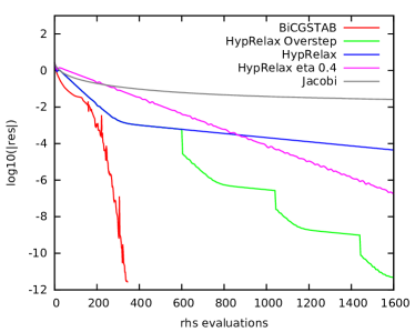
Figure 3: Poisson equation, FD method. Convergence of the residual with the number of right-hand-side evaluations. Shown is a comparison between different methods for $N=101$ in two dimensions.

A key question is how efficient hyperbolic relaxation is compared to other methods. In Fig. 3, we show a comparison of different methods for a two-dimensional example with $N=101$ points. The methods considered are hyperbolic relaxation as above, the standard Jacobi iteration Press et al. (2007), and the BiCGSTAB method as an example for a Krylov subspace method Barrett et al. (1993). Also included are two additional variants of hyperbolic relaxation. In these examples $\Delta t=1.0\Delta x$ for RK4 in 2d.

Referring to Fig. 3, the Jacobi method shows the slowest convergence. Reducing the residuum of the 2d Poisson equation by a factor $10^{-p}$ requires $n\approx\frac{1}{2}pN^{2}$ iterations on a $N\times N$ grid Press et al. (2007). For a 2d grid with $V=N^{2}$ degrees of freedom, the operation count is therefore $O(V^{2})=O(N^{4})$, compared to $O(N^{3})$ for optimal SOR and $O(V\log V)$ for multigrid methods. Hyperbolic relaxation with $O(V)\times O(N)=O(N^{3})$, as demonstrated in Fig. 2, is therefore a reasonable candidate for further consideration. In the concrete example, the Jacobi method is significantly slower than hyperbolic relaxation, but the Jacobi method is usually not considered as a stand-alone method.

For this simple comparison, the BiCGSTAB method is used without a preconditioner, but the Laplace operator leads to a sufficiently well conditioned operator such that convergence is fast nevertheless, compared to the other methods considered here. There is an initial phase of relatively slow convergence, but once the trial solution is sufficiently close to the final answer, convergence becomes much faster.

Remarkably, hyperbolic relaxation does about as well as BiCGSTAB during the first phase. However, convergence slows down after the shorter wavelengths have been damped and errors due to larger wavelength remain. We have considered three ideas to improve the convergence of hyperbolic relaxation for long wavelengths. Not shown here is the multi-level refinement strategy which we employ in the bamps code, see Sec. III.4.

As an immediate application of the mode analysis of Sec. II.3, we introduced the damping parameter $\eta$, which for the basic experiments so far was set to $\eta=1$. Also shown in Fig. 3 is the result for $\eta=0.4$, which is slower than $\eta=1$ initially, but faster for later iterations. This effect is related to the size $L$ of the box. It seems possible to construct a dynamically adjusted damping $\eta(t)$. Similar results hold for the parameter $b$ in (30). The velocity associated with the largest wave number $k$ scales with $\sqrt{b}$ but is independent of $\eta$, so for optimal performance the Courant factor has to be adjusted for the version with $b$ but can be kept constant for the version with $\eta$.

We also experimented with a “one-step overrelaxation” method (as opposed to successive overrelaxation). This is based on the observation that after the initial propagation/damping phase of hyperbolic relaxation, the second time derivative of $\phi$ becomes significantly smaller than the first time derivative, $\partial_{t}^{2}\phi\ll\partial_{t}\phi$. Hence it seems promising to attempt a linear extrapolation in time. The curve labeled “overstep” in Fig. 3 is obtained by searching every few iterations for the time step $\Delta T=\lambda\Delta t$ that minimizes the global residual of $\phi_{new}=\phi+\Delta T\,F(\phi)$, where $F$ is the update suggested by the time stepping algorithm (e.g. RK4). This is similar to various other 1d step-size optimizations. For the example considered here (but also for $\rho\neq 0$ as below), the late time solution of hyperbolic relaxation is sufficiently regular that indeed an appropriate global $\Delta T$ can be found. The overstep algorithm only accepts improvements by a given factor, say 10 (we tried 2 to 1000). After the adjustment the solution is disturbed but converges again with the typical speed for shorter wavelengths to a new regular state, so in the optimal case the overall convergence rate approaches that of the fast phase of hyperbolic relaxation.

The main points regarding the convergence rate of hyperbolic relaxation as shown in Fig. 3 are that the method works out-of-the-box and that its performance falls somewhere between Jacobi and BiCGSTAB. There seems to be quite some potential for accelerating the convergence rate of hyperbolic relaxation. From the point of view of solving elliptic equations with a code designed for hyperbolic equations, note that hyperbolic relaxation is “only” slower by a factor of about 5 (to reach a residual of $10^{-9}$ in this example) than a standard method like BiCGSTAB, which however may not be readily available.

IV.2 Poisson Equation – Pseudospectral Method

To test the hyperbolic relaxation elliptic solver we start by solving Poisson’s equation,

$$\Delta\psi-\rho=0\,,$$ (63)

in spherical symmetry, i.e. $\rho=\rho(r)$, $r=\sqrt{x^{i}x_{i}}$. To solve this equation we choose the hyperbolic relaxation system

$$\partial_{t}\psi =\delta^{ij}\partial_{i}r_{j}-\rho\,,$$ (64)

$$\partial_{t}r_{i} =\partial_{i}\psi-r_{i}\,.$$ (65)

For our first test we take $\rho$ to be smooth, i.e. it is infinitely often continuous differentiable,

$$\rho=\rho_{0}\left(\frac{-6}{R^{2}}+\frac{4r^{2}}{R^{4}}\right)e^{-r^{2}/R^{2}}\,,$$ (66)

where $R$ and $\rho_{0}$ are non-zero parameters. For this $\rho$ Poisson’s equation has the solution

$$\psi_{\rm analytic}=\rho_{0}e^{-r^{2}/R^{2}}\,.$$ (67)

At the boundary a falloff in $\psi$ compatible with this solution is obtained by imposing the Robin boundary condition $\partial_{r}\psi=s^{i}\partial_{i}\psi={-2r}\psi/{R^{2}}$.

For our second test we take a non-smooth $\rho$ that corresponds to a homogeneously charged sphere, which is like a toy model for stars. The density $\rho$ is then given by

$$\rho=\begin{cases}\rho_{0}&\text{ if }r\leq R\\ 0&\text{ if }r>R\,,\end{cases}$$ (68)

for which the Poisson equation has the solution

$$\psi_{\rm analytic}=\rho_{0}\begin{cases}\frac{r^{2}}{6}-\frac{R^{2}}{2}&\text{ if }r\leq R\\ -\frac{R^{3}}{3r}&\text{ if }r>R\,.\end{cases}$$ (69)

Again we impose Robin boundary conditions according to the falloff of this solution, i.e. $\partial_{r}\psi=s^{i}\partial_{i}\psi=-\psi/r$.

In our tests we place the outer boundary at radius of 10 and and we divide the grid into a total of eight subpatches, where the inner five extend over the interval $[0,5]$ and the outer three, having a coarser resolution, extend over $[5,10]$. The parameters determining $\rho$ are chosen to be $R=5$ and $\rho_{0}=1$. For the non-smooth case special care has to be taken to ensure convergence. In particular we chose the grid such that the discontinuity lies at a boundary of subpatch, ensuring second order convergence. In both test cases the relaxed solution converges with the number of grid points to the analytical solution. To investigate the convergence we have to make sure that the solution is completely relaxed on every resolution. This is achieved by choosing in Eq. (59) $c=0.0001$. In Fig. 4 we report the absolute difference between the analytical and numerical solution integrated over the outermost subpatch. We note however that the convergence behavior is the same on all other subpatches. As expected we find the error of the numerical solution to decrease exponentially with the number of points for the smooth $\rho$ from Eq. (66). For the non-smooth $\rho$ of Eq. (68), we only get a convergence order of approximately two, which is the expected convergence order for discontinuous $\rho$. Of course this is not very efficient for a spectral method. For non-smooth right-hand sides it might be preferable to increase the number of subpatches (h-refinement) instead of the number of collocation points per subpatch.

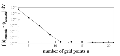
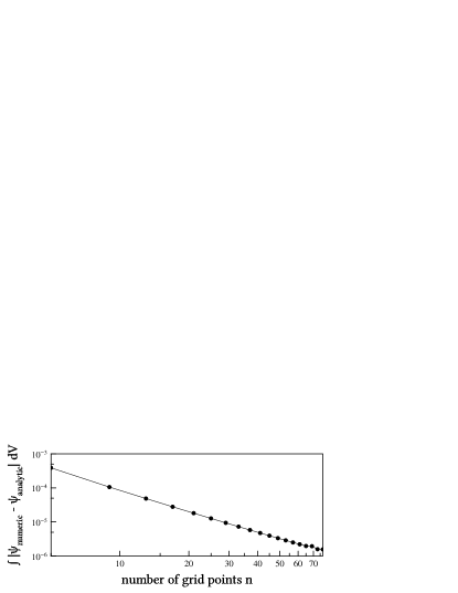
Figure 4: Convergence L1-norm of the difference between the analytical and the numerical solution. Upper plot: for smooth $\rho$ (Eq. (66)). Lower plot: for non-smooth $\rho$ (Eq. (68)). Note that in the upper plot only the error axis is logarithmic, while in the lower plot both axes are logarithmic.

In Fig. 5 we investigate how the L1-norm of different quantities, that can be used to approximate the error, progresses during the relaxation process. First we observe that the difference to the analytical solution decreases even when the computed residual, given by left-hand side of Eq. 63, is already leveling off. This is especially remarkable for the non-smooth case, where the residual itself is not converging at all. For the smooth case we secondly observe that after refining the grid the norm of right-hand side of Eq. (64) practically continues at the same level as before. The norm of the residual on the other hand drops quickly after refining, reaching the right-hand sides level until again the discretization limit is reached. These observations suggest that for problems with smooth solutions it is preferable to relax for longer on the coarse grid. For problems with non-smooth solutions, however, more new error develops during each refinement and thus refining for longer on the coarse grid is not paying off. Furthermore, it is preferable to increase the grid resolution faster.

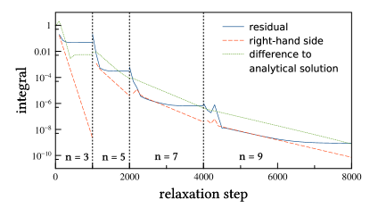
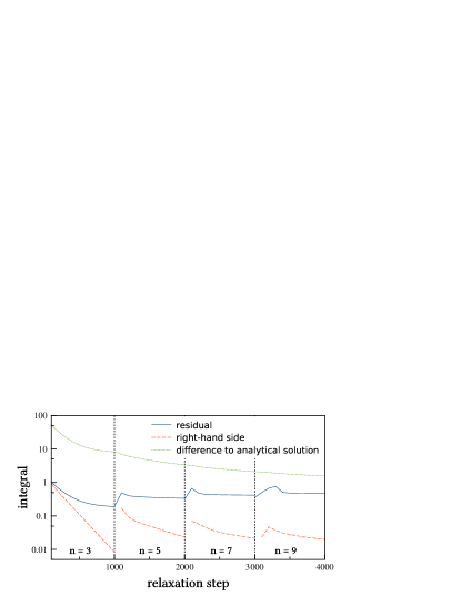
Figure 5: Progression of the L1-norm of different error quantities during of the relaxation process for the Poisson equation. Vertical dashed lines indicate transitions to a finer grid. The respective error quantities are: blue solid line: residual, defined as left-hand side of Eq. 63, orange dashed line: right-hand side of Eq. 64, green dotted line: difference to the analytical solution. Upper plot: for smooth $\rho$ (Eq. (66)). Lower plot: for non-smooth $\rho$ (Eq. (68)).

As a last simple test, we investigated the behavior in the case of non-unique solutions. For this we took the smooth $\rho$ from Eq. (66) and imposed the Neumann boundary condition $\partial_{r}\psi=0$, for which multiple solutions differing only by an additive constant exist. We find that after some relaxation the right hand side of Eq. (64) becomes approximately constant in space. From this point on the solution is no longer improving, since only constant terms, which do not improve the residual of Eq. (63), are added.

V Application to Initial Data for General Relativity

V.1 The Extended Conformal Thin-Sandwich Equations

In numerical relativity one usually decomposes the spacetime metric $g_{ab}$ into a temporal and spatial part in the form

$$g_{ab}dx^{a}dx^{b}=-\alpha^{2}dt^{2}+\gamma_{ij}(dx^{i}+\beta^{i}dt)(dx^{j}+\beta^{j}dt)\,,$$ (70)

where $\alpha$ is called the lapse, $\beta^{i}$ the shift and $\gamma_{ij}$ the spatial metric. The equations of motion in general relativity are subject to constraint equations, which have to be solved before the spacetime is evolved numerically. A popular formulation of the constraint equations is given by the extended conformal thin-sandwich (XCTS) equations Baumgarte and Shapiro (2010); Tichy (2017) in which the spatial metric is decomposed into a conformal factor $\psi$ and a spatial conformal metric $\bar{\gamma}_{ij}$ as $\gamma_{ij}=\psi^{4}\bar{\gamma}_{ij}$. In the XCTS framework the constraint equations take the form

$$\bar{D}^{j}\bar{D}_{j}\psi= \frac{\psi}{8}\bar{R}-\psi^{5}\left(2\pi\rho-\frac{K^{2}}{12}+\frac{1}{8}A_{ij}A^{ij}\right)\,,$$ (71)

$$\begin{split}\bar{D}^{j}\bar{D}_{j}\beta^{i}=&-\frac{1}{3}\bar{D}^{i}\bar{D}_{j}\beta^{j}-\bar{R}\indices{{}^{i}_{j}}\beta^{j}+16\pi\alpha\psi^{4}J^{i}\\ &+(\bar{D}^{i}\beta^{j}+\bar{D}^{j}\beta^{i}-\frac{2}{3}\bar{\gamma}^{ij}\bar{D}_{k}\beta^{k})\\ &\quad\cdot\bar{D}_{j}\ln(\alpha\psi^{-6})\\ &-\alpha\psi^{-6}\bar{D}_{j}(\alpha^{-1}\psi^{6}\partial_{t}\bar{\gamma}^{ij})+\frac{4}{3}\alpha\bar{D}^{i}K\,,\end{split}$$ (72)

$$\begin{split}\bar{D}^{j}\bar{D}_{j}(\alpha\psi)=&\alpha\psi^{5}\left(\frac{7}{8}A_{ij}A^{ij}+\frac{5}{12}K^{2}+2\pi(\rho+2J)\right)\\ &-\psi^{5}(\partial_{t}-\beta^{j}\bar{D}_{j})K+\frac{1}{8}\alpha\psi\bar{R}\,.\end{split}$$ (73)

Here $\bar{D}_{i}$ is the covariant derivative compatible with the conformal metric $\bar{\gamma}_{ij}$, $\bar{R}\indices{{}_{i}{}_{j}}$ is the Ricci tensor of $\bar{\gamma}_{ij}$ and $\bar{R}$ is the corresponding Ricci scalar. The tensor $A_{ij}$ is the tracefree part of the extrinsic curvature $K_{ij}$ and $K$ is the trace of $K_{ij}$. The matter source terms are defined as the following contractions of the energy-momentum tensor $T_{ab}$: $\rho=T_{ab}n^{a}n^{b}$, $J^{i}=-T_{ab}\gamma^{ia}n^{b}$ and $J=\gamma^{ab}T_{ab}$, where $n^{a}$ is the timelike vector normal to the spatial hypersurface $n^{a}=(1/\alpha,-\beta^{i}/\alpha)$. For conformal quantities (denoted by a bar) the conformal spatial metric $\bar{\gamma}^{ij}$ lowers and raises indices and for unbarred quantities the physical spatial metric $\gamma^{ij}$ is used. In the XCTS equations $\bar{\gamma}_{ij}$, $\partial_{t}\bar{\gamma}_{ij}$, $K$ and $\partial_{t}K$ are given functions, depending on the type of initial data you want to construct.

In Eq. (73) the product $\alpha\psi$ is taken as one variable. For our computations we rewrite this equation with the help of Eq. (71) as

$$\begin{split}\bar{D}^{j}\bar{D}_{j}\alpha=&-\frac{2}{\psi}(\bar{D}^{j}\alpha)(\bar{D}_{j}\psi)-\psi^{4}(\partial_{t}-\beta^{j}\bar{D}_{j})K\\ &+\alpha\psi^{4}\left(A_{ij}A^{ij}+\frac{K^{2}}{3}+4\pi(\rho+J)\right)\,,\end{split}$$ (74)

so we can solve directly for $\alpha$. We have tested our elliptic solver with both versions and found them to work equally well in our applications. In the following we investigate the XCTS system with our replacement for the lapse equation, but the analysis would be exactly the same for the original system.

The principal part of the XCTS equations is given by

$$\begin{pmatrix}\bar{\gamma}^{kj}&0&0\\ 0&\bar{\gamma}^{kj}\delta^{l}_{i}+\frac{1}{3}\bar{\gamma}^{lk}\delta^{j}_{i}&0\\ 0&0&\bar{\gamma}^{kj}\\ \end{pmatrix}\partial_{k}\partial_{j}\begin{pmatrix}\psi\\ \beta^{i}\\ \alpha\\ \end{pmatrix}\,.$$ (75)

The principal part is coupled only between the components of $\beta^{i}$. Thus we can carry out the hyperbolicity analysis independently for $\psi$, $\alpha$ and $\beta^{i}$.

The metric to lower and raise spatial indices in the hyperbolic relaxation method is in principal arbitrary, but for the XCTS equations we use the conformal metric $\bar{\gamma}_{ij}$, because this choice simplifies the following formulas considerably. Another peculiarity is the fact that spatial indices and field indices “mix”, but in general they are lowered and raised by different metrics. Therefore we do not lower and raise field indices and instead write the Euclidian metric explicitly.

For the conformal factor part we have in the hyperbolic relaxation system $a^{ij}=\bar{\gamma}^{ij}$ and we choose $b\indices{{}^{i}_{j}}=\delta^{i}_{j}$. Here we have suppressed the field indices, because we only have a single field $\psi$. The characteristic variables and speeds of the hyperbolic relaxation system of the $\psi$ part are then given by

$$\hat{u}^{0}_{j} =r_{j}-s_{j}s^{i}r_{i}^{(\psi)}\,,~{}~{}~{}~{}~{}~{}~{}~{}~{}~{}~{}\lambda^{0}_{i}=0\,,$$ (76)

$$\hat{u}^{\pm} =\psi\pm s^{i}r_{i}^{(\psi)}\,,~{}~{}~{}~{}~{}~{}~{}~{}~{}~{}~{}~{}~{}\,\lambda^{\pm}=\pm 1\,,$$ (77)

where $r_{i}^{(\psi)}$ is the reduction variable for $\psi$.

The lapse part has exactly the same principal part, so we have identical $a^{ij}$ and $b\indices{{}^{i}_{j}}$ and the characteristics are

$$\hat{u}^{0}_{j} =r_{j}-s_{j}s^{i}r_{i}^{(\alpha)}\,,~{}~{}~{}~{}~{}~{}~{}~{}~{}~{}~{}\lambda^{0}_{i}=0\,,$$ (78)

$$\hat{u}^{\pm} =\alpha\pm\bar{s}^{i}r_{i}^{(\alpha)}\,,~{}~{}~{}~{}~{}~{}~{}~{}~{}~{}~{}~{}~{}\,\lambda^{\pm}=\pm 1\,,$$ (79)

with $r_{i}^{(\alpha)}$ being the reduction variable for $\alpha$.

In the derivation of the hyperbolic relaxation equations we labeled the fields with lower indices. For the shift however we use upper indices here and thus one has to be careful, not to confuse the indices. Therefore, we introduce auxiliary fields $\phi_{\alpha}$ with

$$\beta^{\alpha}=\delta^{\alpha\beta}\phi_{\beta}\,.$$ (80)

Substituting $\beta^{\alpha}$ we obtain for the principal part of the shift equations

$$a\indices{{}^{i}{}^{j}{}^{\beta}_{\alpha}}\partial_{i}\partial_{j}\phi_{\beta}=(\bar{\gamma}^{ij}\delta^{\beta}_{\alpha}+\frac{1}{3}\bar{\gamma}^{i\epsilon}\delta_{\epsilon\alpha}\delta^{j\beta})\partial_{i}\partial_{j}\phi_{\beta}\,.$$ (81)

We take $b\indices{{}^{i}_{j}{}^{\beta}_{\alpha}}$ to be the inverse of $a$ (as defined in section II.4), $b\indices{{}^{i}_{j}{}^{\beta}_{\alpha}}=\delta^{i}_{j}\delta^{\beta}_{\alpha}-\frac{1}{6}\delta^{i\beta}\delta_{j\alpha}$ . The characteristic variables and speeds for this part of the hyperbolic relaxation system are then given by

$$\hat{u}^{0}_{j\gamma} =r_{j\gamma}-b\indices{{}^{s}_{j}{}^{\epsilon}_{\gamma}}({b\indices{{}^{s}_{s}}}^{-1})\indices{{}^{\alpha}_{\epsilon}}s^{i}r_{i\alpha}$$ (82)

$$=r_{j\gamma}-s_{j}s^{i}r_{i\gamma}+\frac{1}{5}(\delta_{j\gamma}-s_{j}s^{l}\delta_{l\gamma})s_{k}\delta^{k\alpha}s^{i}r_{i\alpha}\,,$$ (83)

$$\lambda^{0}_{i\gamma} =0\,,$$ (84)

$$\hat{u}^{\pm}_{\gamma} =\phi_{\gamma}\pm a\indices{{}^{s}{}^{i}{}^{\alpha}_{\gamma}}r_{i\alpha}~{}~{}~{}~{}~{}~{}$$ (85)

$$=\phi_{\gamma}\pm(s^{i}r_{i\gamma}+\frac{1}{3}s^{\epsilon}\delta_{\epsilon\gamma}\delta^{j\alpha}r_{j\alpha})\,,$$ (86)

$$\lambda_{\gamma}^{\pm} =\pm 1\,,$$ (87)

where the $r\indices{{}_{i}{}_{\alpha}}$ denote the reduction variables for the auxiliary fields $\phi_{\alpha}$

At the domain boundary we want the solution to fall off like the Schwarzschild solution, i.e. $\psi=\frac{a}{r}+1$ and $\alpha=\frac{b}{r}+1$. This ansatz gives rise to the following Robin boundary conditions

$$\partial_{s}\psi|_{\partial\Omega}=\frac{1-\psi}{r}\,,~{}~{}~{}~{}~{}~{}\partial_{s}\alpha|_{\partial\Omega}=\frac{1-\alpha}{r}\,.$$ (88)

For the shift we likewise impose a radial falloff by the Robin condition

$$\partial_{s}\beta^{i}|_{\partial\Omega}=\frac{\beta^{i}}{r}\,.$$ (89)

As an initial guess we always use the flat space solution, i.e. $\psi=1$, $\alpha=1$, $\beta^{i}=0$. Of course an initial guess, that is a good approximation to the solution is always the preferred start for the relaxation, since it will take less time to relax to the solution or might be necessary to relax at all. However we find our simple initial guess to work well and it demonstrates in a nice way the high robustness of the hyperbolic relaxation method exhibited in our experiments.

V.2 Scalar Field

The energy-momentum tensor for a scalar field $\phi$ is given by

$$T_{ab}=\nabla_{a}\phi\nabla_{b}\phi-\frac{1}{2}g_{ab}\left(\nabla_{c}\phi\nabla^{c}\phi+m^{2}\phi^{2}\right)\,,$$ (90)

where $\nabla$ denotes the covariant derivative compatible with $g_{ab}$. We consider conformally flat moment-of-time-symmetry initial data, i.e. $\bar{\gamma}_{ij}=\delta_{ij}$, $n^{a}\nabla_{a}\phi=0$, $\partial_{t}\bar{\gamma}_{ij}=0$ and maximal slicing $K=0$, $\partial_{t}K=0$. This yields for the matter quantities

$$\rho =\frac{1}{2}\gamma^{ij}(\partial_{i}\phi)(\partial_{j}\phi)+\frac{1}{2}m^{2}\phi^{2}\,,$$ (91)

$$J^{i} =0\,,$$ (92)

$$J =-\frac{1}{2}\gamma^{ij}(\partial_{i}\phi)(\partial_{j}\phi)-\frac{3}{2}m^{2}\phi^{2}\,.$$ (93)

For a massless scalar field ($m=0$) the solutions for lapse and shift are trivially given by $\alpha=1$ and $\beta^{i}=0$ and we only have to determine the conformal factor $\psi$ by solving Eq. (71), now taking the form

$$0=\delta^{ij}\partial_{i}\partial_{j}\psi+\pi\psi\delta^{ij}(\partial_{i}\phi)(\partial_{j}\phi)\,.$$ (94)

For a massive scalar field ($m\neq 0$) one would have either have to solve additionally for the lapse or one gives up the requirement on $\partial_{t}K$. For the scalar field we choose radially symmetric, smooth initial data of the form

$$\phi(r)=p\left(\tanh\frac{r}{\sigma}-\tanh\frac{r}{\sigma}\right)\,,$$ (95)

where $\sigma$ and $p$ are free parameters, that we choose for our test to be $\sigma=1$ and $p=0.1$.

The computational domain is divided into eight subpatches, where the inner five subpatches are of smaller extent to improve the resolution near the center. In Fig. 6 we show the numerical solution for the conformal factor and the absolute value of the residual of Eq. (71) for a resolution of 21 collocation points per subpatch. A general feature that can be observed in the residual are spikes at the boundary of subpatches, which are expected for quantities involving first and second derivatives in a discontinuous Galerkin approximation.

We also investigate how the solution converges with increasing resolution. For this purpose we look at the Chebyshev coefficients and investigate their convergence against the coefficients of a high resolution solution. In Fig. 7 we present the convergence behavior of the lowest Chebyshev mode $C(0,0,0)$ against its value for a resolution of 31 collocation points. We observe an exponential convergence until we hit machine precision at around a resolution of 25 collocation points per subpatch.

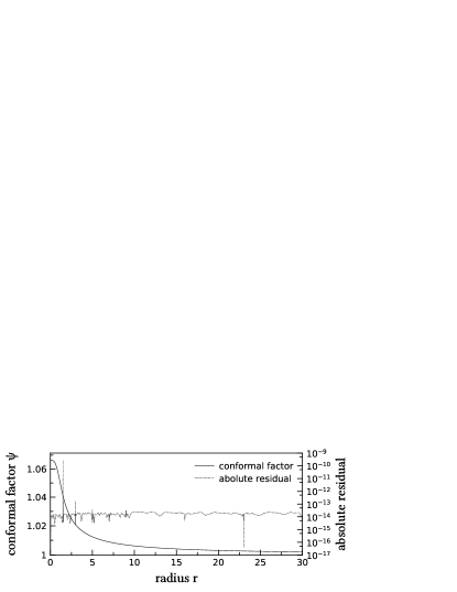
Figure 6: Steady state at a resolution of 21 collocation points per subpatch for the initial data of the scalar field. Solid line: conformal factor. Dashed line: residual for conformal factor, as given by the right-hand side of Eq. (94).

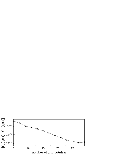
Figure 7: Convergence of the lowest Chebyshev coefficient $C(0,0,0)$ at the innermost subpatch for the initial data of the scalar field. The system is relaxed for different numbers of collocation points. The plot shows the absolute value of the difference between the Chebyshev coefficient at the highest resolution (31 collocation points) and its value for $n$ collocation points per subpatch. For $n=25$ the difference is zero within machine precision and is therefore not displayed on the logarithmic axis.

V.3 Tolman-Oppenheimer-Volkoff Star

The energy-momentum tensor of a perfect fluid is given by

$$T_{ab}=(\epsilon+p)u_{a}u_{b}+pg_{ab}\,,$$ (96)

where $\epsilon$ is the proper energy density, $p$ the fluid pressure and $u_{a}$ the fluid four-velocity. The Tolman-Oppenheimer-Volkoff (TOV) solution Moldenhauer (2012); Moldenhauer et al. (2014); Baumgarte and Shapiro (2010) is a static radially symmetric solution to general relativity, thus we have $u_{a}=(\alpha,0)$, $\bar{\gamma}_{ij}=\delta_{ij}$, $\partial_{t}\bar{\gamma}_{ij}=0$ and we consider again maximal slicing $K=0$, $\partial_{t}K=0$. The matter quantities then become

$$\rho=\epsilon\,,~{}~{}~{}~{}~{}~{}J^{i}=0\,,~{}~{}~{}~{}~{}~{}J=3p\,.$$ (97)

We assume for our tests a polytropic equation of state and express the matter quantities in terms of the specific enthalpy $h$,

$$\rho =\left(1+\frac{n(h-1)}{1+n}\right)\left(\frac{h-1}{\kappa(1+n)}\right)^{n}\,,$$ (98)

$$J =3\kappa\left(\frac{h-1}{\kappa(1+n)}\right)^{n+1}\,,$$ (99)

where $\kappa$ is the adiabatic constant and $n$ is the polytropic index. The Euler equation follows from energy-momentum conservation, i.e. for a fluid with temperature $T=0$

$$u^{a}(\nabla_{a}(hu_{b})-\nabla_{b}(hu_{a}))=0\,,$$ (100)

which has to be satisfied in addition to the XCTS equations. For our assumptions the Euler equation is satisfied for $\alpha h=const.$ and thus specifying the specific enthalpy at the origin yields

$$h(r)=\begin{cases}\frac{h(0)\alpha(0)}{\alpha(r)}&\text{ if }\alpha(r)<h(0)\alpha(0)\\ 1&\text{ else }\end{cases}\,.$$ (101)

We can immediately get the solution for the shift $\beta^{i}=0$ and are left with solving Eq. (71) and (74) of the XCTS system.

For our test we choose an adiabatic constant of $\kappa=123.6489$ and a polytropic index of $n=1$ and the enthalpy in the star’s center is set to $h(0)=1.2$. We present the solution for the conformal factor and the lapse in Fig. 8 and investigate the convergence of their lowest Chebyshev modes in Fig. 9. The residuals are large at the stellar surface, i.e. where $\alpha(r)=h(0)\alpha(0)$. This is caused by the fact that the matter terms are not smooth at this point, which can be seen in the kink in the specific enthalpy $h$. As for the non-smooth right-hand sides discussed in Sec. IV.2, we have to make sure that the kink lies at a subpatch boundary. By trial and error we find the stellar surface for the above parameters to be located at $r=9.7098$ and we place a subpatch boundary at this position “by hand”. A more sophisticated method is to fit coordinates automatically to the stellar surface Tichy (2009). This however is beyond the scope of this paper as we here want to focus on applications of the hyperbolic relaxation method. In contrast to what we observed in the non-smooth case for the Poisson equation, here the Chebyshev coefficients converge exponentially despite the kink in the specific enthalpy. The convergence rate however is much smaller than that observed for the initial data of the scalar field.

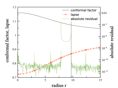
Figure 8: Steady state at a resolution of 27 collocation points per subpatch for the initial data of the TOV star. Solid line: conformal factor. Orange dashed line with markers: lapse. Green dash-dotted line: absolute value of the residual for the conformal factor, as given by the right-hand side of Eq. (71). Vertical dashed line: position of the stellar surface.

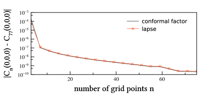
Figure 9: Convergence of the lowest Chebyshev coefficient as in Fig. 7 for the initial data of the TOV star. The highest resolution used in these runs was 77 collocation points per subpatch.

V.4 Neutron Star Binaries

For the construction of neutron star binary initial data we follow the scheme of Moldenhauer et al. (2014) using the constant three-velocity approximation. However, to solve the XCTS equations we do not rely on iterating the solution of the equations for the conformal factor, lapse and shift separately, but instead we solve for all variables simultaneously relaxing the complete XCTS system, which accelerates the solution process. This is a feature that most solvers for this type of initial data do not provide, and it could turn out to be an advantage of our method. Furthermore, we do not start with superposed (boosted) TOV solutions, but instead start with a flat metric $\psi=1$, $\alpha=1$, $\beta^{i}$, as discussed at the end of Sec. V.1.

For our test we consider equal mass neutron stars with a specific enthalpy of $h=1.01$ in each of their centers and a separation of 80. For the equation of state we choose again $\kappa=123.6489$ and $n=1$. The stars’ centers are located at the $z$-axis and their velocities are parallel to the $x$-axis. We construct in initial data for irrotational stars on a quasicircular orbit. In Fig. 10 we present results for the conformal factor, lapse, the $x$-component of the shift, the residual of the conformal factor equation. As for the TOV star initial data, the residuals are biggest on those subpatches which contain the stellar surfaces, where the matter fields are not smooth.

Because we are not using surface-fitted coordinates Bonazzola et al. (1998); Ansorg (2007); Tichy (2009) we can not place the stellar surface at a subpatch boundary, and thus no high-order convergence in the norm of the residuals can be seen with increasing number of collocation points. Although this may be a disadvantage for studies of initial data per se, the situation changes if the goal is evolution of the data. Since in an actual evolution of this data surface-fitted coordinates are normally not retained, the high accuracy of initial data with surface-fitted coordinates will be lost relatively quickly anyway. On the other hand, methods like Tichy (2009) require expensive iterations to determine the surface fitting coordinates as part of the solution process, so any method which works without special coordinates is more efficient in that part of the algorithm. In fact, part of the motivation for the multigrid method in Moldenhauer et al. (2014) was to construct a solver which works on a general Cartesian grid without surface-fitting coordinates. The hyperbolic relaxation method achieves the same goal.

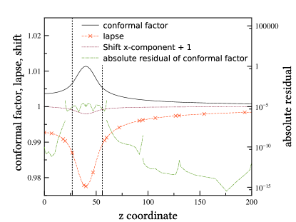
Figure 10: Steady state at a resolution of 11 collocation points per subpatch for the initial data of a binary neutron star system. We show data along the positive $z$-axis. The values on the negative axis are symmetric (anti-symmetric for the shift component $\beta^{x}$). Solid line: conformal factor. Orange dashed line with markers: lapse. Purple dotted line: $x$-component of the shift, shown here with an offset of one for clarity. Green dash-dotted line: absolute value of the residual for the conformal factor, as given by the right-hand side of Eq. (71). Vertical dashed line: position of the stellar surface.

VI Conclusions

The most common types of relaxation methods are based on the famous Gauss-Seidel method, which can be motivated by rewriting the problem as a parabolic diffusion equation that relaxes from an initial guess to the solution of the elliptic PDE. In this paper we investigated a new class of relaxation methods, which are not based on parabolic, but rather on hyperbolic PDEs. In the literature hyperbolic relaxation is usually discussed from the point of view that a hyperbolic equation is given which may contain physical or numerical dissipation terms. In this work we assume that an elliptic equation is given, which is extended to a hyperbolic relaxation equation for the purpose of solving the elliptic equation. In some respect, hyperbolic relaxation might actually be as well suited for the solution of elliptic PDEs as parabolic relaxation.

We investigated how a hyperbolic relaxation method (HypRelax) can be constructed for a general class of second order, non-linear elliptic PDEs and discussed its structure and properties. A discussion of the general hyperbolicity properties has been carried out and three specific choices for the relaxation were discussed. For the special case of the Laplace equation, a mode analysis revealed that there is a critical wavenumber at which the qualitative behavior of the modes is changing. It has also been seen that at low wavenumber the damping rate approaches that of the Jacobi method from above. It is an interesting topic for the future how the specific choice of the relaxation system (choice of $b\indices{{}^{j}_{i}{}^{\beta}_{\alpha}}$) affects the behavior of the modes, how that choice can be optimized, and what would be the modes for more general elliptic equations.

Furthermore, we have shown how the standard types of boundary conditions – Dirichlet, Neumann and Robin boundary conditions – can be implemented within the hyperbolic relaxation framework.

With regard to advantages, hyperbolic relaxation shares with several other methods the feature that it is “matrix free”, i.e. it is possible to avoid the construction of an explicit matrix form by applying the differential operator directly. Also note that as in Jacobi methods, non-linear equations can be treated without linearization, avoiding the additional work of e.g. outer Newton-Raphson iterations.

The ease of implementation is a key feature of hyperbolic relaxation. In the past, we implemented a parallel geometric multigrid method for the BAM and Cactus codes Brandt and Brügmann (1997); Alcubierre et al. (2001); Brügmann et al. (2008); Moldenhauer et al. (2014). We also interfaced BAM to the hypre package hyp ; Ansorg et al. (2004) for access to a variety of elliptic solvers, in particular algebraic multigrid. To avoid complicated dependencies, some of the black hole initial data was later computed with a stand-alone Newton-Raphson method, or even with the direct solver in MATLAB for numerical stability Dietrich and Brügmann (2014). Our current production runs for a wide range of binary neutron star initial data rely on the sophisticated spectral solver sgrid Tichy (2009, 2012); Dietrich et al. (2015). Unsurprisingly, compared to the various approaches just mentioned, hyperbolic relaxation is very straightforward to implement given a hyperbolic evolution code.

We have implemented the hyperbolic relaxation method in our spectral hyperbolic evolution code bamps Brügmann (2013); Hilditch et al. (2016) (and in a finite differencing test code). For numerical tests we have applied it to Poisson’s equation, and we also presented applications to numerical relativity initial data, where we have seen a high robustness with respect to the choice of an initial guess and regarding the simultaneous solution of the XCTS equations. Given the complexity of binary neutron star initial data and the correspondingly involved numerical methods that have been developed to solve these elliptic equations, e.g. Tichy (2017) and references therein, it is a non-trivial result that the hyperbolic relaxation method results in a robust and quite efficient elliptic solver.

We have seen that the damping rate at low wavenumbers is comparable to that of the Jacobi method and thus very low. In this study we were most interested in the basic properties of the hyperbolic relaxation method and thus we focussed on a simple scheme of successive refinement, but there exist more sophisticated accelerators, in particular multigrid methods, that could be implemented also for a hyperbolic relaxation scheme. Another possible extension of our hyperbolic relaxation implementation would be an adaptive mesh refinement scheme, for which we see two main advantages. First of all, there are the usual savings due to optimized local resolution, and secondly, since we want to use the solution of the elliptic equation as initial data, this will provide us with a grid that should already be well adapted to the evolution of the obtained data. Another idea is to employ adaptive time stepping, for which however special care would be required to keep the numeric scheme stable.

With regard to initial data for neutron stars, one of the potential problems is the lack of differentiability at the surface of the stars. We were prepared to evolve the neutron star data with a high-resolution shock-capturing method, but in fact this was not necessary given the strong diffusion of the equations. In applications where the wave propagation feature is important, shock handling may be a feature that comes at no extra cost assuming that there is an evolution code providing the appropriate methods.

The investigations of this paper can only serve as a first step in the exploration of this potentially promising branch of new relaxation methods. Hyperbolic relaxation might become with further study, and in particular in combination with acceleration methods, the basis of an alternative numerical solution method for elliptic equations.