Measuring technological complexity - Current approaches and a new measure of structural complexity

Abstract

The paper reviews two prominent approaches for the measurement of technological complexity: the method of reflection and the assessment of technologies’ combinatorial difficulty. It discusses their central underlying assumptions and identifies potential problems related to these. A new measure of structural complexity is introduced as an alternative. The paper also puts forward four stylized facts of technological complexity that serve as benchmarks in an empirical evaluation of five complexity measures (increasing development over time, larger R&D efforts, more collaborative R&D, spatial concentration). The evaluation utilizes European patent data for the years 1980 to 2013 and finds the new measure of structural complexity to mirror the four stylized facts as good as or better than traditional measures.

1 Introduction

The complexity of technologies is seen as crucial explanatory dimension of technological development and economic success Romer, (1990); Dalmazzo, (2002). Hidalgo and Hausmann, (2009) argue that country’s economic development is shaped by its ability to successfully engage in complex economic activities and technologies. Both Sorenson, (2005) and Balland and Rigby, (2017) show that few cities are capable of mastering complex technologies that lay the foundation for their future growth.

Despite its theoretical relevance and an increasing empirical interest, measuring the complexity of technologies empirically is a complicated issue, as Pintea and Thompson, (2007) note: “We do not have any easy way to measure complexity” [p. 280]. The two most prominent approaches are put forward by Fleming and Sorenson, (2001) and Balland and Rigby, (2017), with the latter transferring the approach of Hidalgo and Hausmann, (2009) for approximating economic complexity to the measurement of technological complexity. The present paper presents both approaches and argues that they build on the assumption of complexity being scarce at their core. Balland and Rigby, (2017) assume technological complexity to be spatially scare, while Fleming and Sorenson, (2001) build on the idea of complex knowledge combinations appearing less frequently than simple ones. It is shown that these assumptions are either theoretically problematic or may induce challenges in the measures’ empirical application.

The paper develops an alternative measure of technological complexity, structural complexity, which does not relate scarcity and complexity. The paper proceeds by empirically evaluating the approaches (and including two variants of the traditional approaches) against four stylized facts of technological complexity (increasing average complexity over time, more collaborative R&D, spatial concentration, and larger R&D efforts). The empirical assessment is made using patent data for Europe between 1990 to 2015. The new measure of structural complexity is shown to match the stylized facts similarly or even better than the traditional measures. Similar to the measure of Fleming and Sorenson, (2001), it is not dependent upon the definition of spatial units.

The paper is structured as follows. The next section discusses the traditional approaches of measuring technological complexity. It also introduces the new measure of structural complexity. Section 3 presents four stylized facts of technological complexity that will serve as benchmarks for the empirical comparison of the traditional and new complexity measures. The set up of the empirical evaluation is subject to Section 4, the results of which are presented and discussed in Section 5. Section 6 summarizes the findings and concludes the paper.

2 Two traditional and one new measures of technological complexity

2.1 (Re-)combinatorial rareness and complexity

Fleming and Sorenson, (2001) approach technological complexity by conceptualizing technological advancement as a search process for knowledge combination. They assume that the difficulty of combining knowledge represents technological complexity, with more difficult combinations being required to advance more complex technologies. Their second assumption relates past knowledge re-combination frequencies to the current difficulty of combinatorial innovation. On this basis, they construct a measure of technological complexity resembling the (in-)frequency of past knowledge combination such that small frequencies, after controlling for their chances of random occurrence in an N/K framework of Kauffmann, (1993), translate into low complexity values. In a follow-up study employing US patent data, they substantiate their results by showing that their measure of technological complexity fits well with inventors’ perceived difficulty of the inventive combination process Fleming and Sorenson, (2004).

However, does the past (in-)frequency of combination really give a clear approximation of the inventive difficulty and thereby of technological complexity? Less frequent combinations may indeed be caused by the difficulty of the according invention process. Yet, it also seems plausible that there is, or has been, little technological or economic interest in such a combination. For instance, it should be relatively easy to integrate the electronic navigation technology used in cars into horse chariots. However, this combination has rarely been realized, if at all, most likely because there is little market potential for it.

2.2 The method of reflection approach

Balland and Rigby, (2017) propose an alternative measure of economic complexity building on the work of Hidalgo and Hausmann, (2009). They transfer the so-called method of reflection used by Hidalgo and Hausmann, (2009) to assess economic complexity to empirically derive a measure of technological complexity. The method of reflection is based on diversity and ubiquity and assumes that technological complexity is spatially scarce. Diversity is the number of distinct technologies in a region and ubiquity the number of regions specialized in a technology. The proposed index of technological complexity yields high values for technology A, when places specialized in A are also specialized in other technologies that few other places are specialized in. Put differently, a technology will be evaluated as being complex when it belongs to a group of technologies few places specialize in and these specializations appear in the same places. Balland and Rigby, (2017) apply this approach to patent data and estimate the complexity of technologies considering the technological specialization of US metropolitan statistical areas. The authors find that regions commonly associated with technological and economic success (e.g., San Jose, Austin, Bay area) are highly specialized in complex technologies.

There are many arguments supporting the idea of complexity being spatially scarce (see also subsection 3). Hidalgo and Hausmann, (2009) argue that in order to be successful in complex activities (e.g. in the development of complex technologies), it requires “nontradable” spatial “capabilities” including “property rights, regulation, infrastructure, specific labor skills” (p. 10570 Hidalgo and Hausmann,, 2009). Similarly, concepts like “learning regions”, “innovative milieu”, and “regional innovation systems” argue that few regions possess location-specific capabilities yielding advantages for technological development (Feldman,, 1994; von Hippel,, 1994; Markusen,, 1996; Florida,, 1995; Camagni,, 1991; Cooke,, 1992). The findings of Sorenson, (2005) add some empirical support to this by showing that 10 to 15 % of industrial agglomeration can be explained by technological complexity.

However, technologies’ spatial distribution may have multiple sources among which complexity is just one. For instance, corporate R&D facilities are known to be located close to public universities Jaffe, 1989b , whose location is largely determined by policy and historical circumstance. The distribution is also impacted by technologies’ geographic diffusion, which depends among others on its degree of maturity, popularity, natural conditions, geographic distances, place of origin, and crucially, economic potential Hägerstrand, (1967); Teece, (1977); Rogers, (1995); Zander and Kogut, (1995). Hence, all these factors that are not related to technological complexity may impact technologies’ spatial distribution and potentially distort the complexity measure.

Two more issues are related to the assumption of spatial scarcity. First, it makes the measure highly endogenous when analyzing spatial phenomena. For instance, endogeneity is likely to arise when the spatial distribution of technologies is explained with their levels of complexity using a complexity measure based on their spatial distribution (see, e.g., Balland and Rigby,, 2017). Crucially, this issue prevents a sound empirical test of the measure’s underlying assumption of complexity being spatially scarce.

Second, as the measure requires a spatial delineation of regions, it becomes conditional on this definition. Put differently, a technology’s complexity may depend on the employed spatial unit, i.e., the size of the regions.

2.3 A measure of structural complexity

Fleming and Sorenson, (2001) base their measure on ideas of complex systems. I follow this line of thinking and start with technological advancement being a knowledge combination process. I also follow their argument of technologies’ complexity being related to the difficulty of combining knowledge pieces in its advancement. Knowledge can be thought of as a “network” of knowledge combination with the nodes being individual knowledge pieces and their combination representing the links. To borrow the example of Hidalgo, (2015), think of an airplane as a specific type of technology. In order to fly, the airplane combines many different knowledge pieces. Crucially, some pieces need to be directly linked in order to function (e.g., wing design and aluminum processing), while others just need to be indirectly related (e.g., electronic navigation and wing design). When representing the airplane as the network of combined knowledge pieces, wing design and aluminum processing are directly linked. In contrast, electronic navigation is only indirectly related, as other knowledge pieces (electronic control systems, mechatronical interfaces, etc.) act as bridges.

In this conception, I propose to use the complexity of this network representing the combinatorial structure of knowledge pieces as a measure of the (airplane) technology’s complexity. That is, the difficulty of combining knowledge is argued to be determined by the precise structure with which knowledge pieces are integrated with each other in innovation processes. Complex structures are more difficult to realize and hence represent more complex technologies. This is motivated by two arguments, one being inspired by the literature on network complexity (Simon,, 1962; Bonchev and Buck,, 2005) in combination with the literature on knowledge relatedness Nooteboom, (2000); Frenken et al., (2007) and the second by information theory Wiener, (1947); Shannon, (1948).

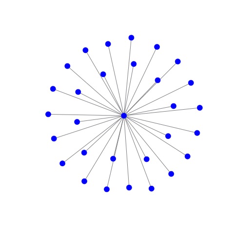
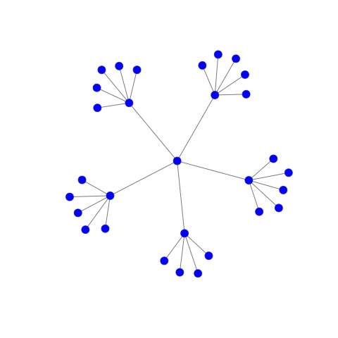
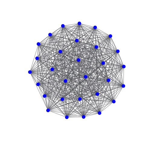
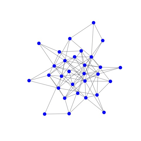
Beginning with the literature on network complexity and knowledge relatedness, Figure 1 shows ideal typical network structures. If the combinatorial network has the shape of a star, it means that all knowledge pieces just need to be combined with a central one. As knowledge piece combinations require some technological / cognitive overlap (Nooteboom,, 2000; Boschma,, 2005), the pieces share some common parts making combination/integration easier. The same reasoning applies to fully connected networks (Complete). Such overlap is lower when multiple central knowledge pieces characterize the combinatorial network (tree structure). In this sense, the network resembles the idea of the knowledge space (see, e.g., Kogler et al.,, 2013; Balland and Rigby,, 2017). The greater knowledge diversity makes such network structures more complex. A tree network implies a modular structure with each module being made of somewhat similar knowledge pieces, which reduces the overall complexity in the network. Such clear-cut modules as in a tree network are less frequent than small-world network structures, which therefore indicate greater knowledge diversity. However, there is still a certain degree of modularity and symmetry, which provides some simplifying patterns. Any of those are lacking in purely random combinatorial structures (Random). Each element is combined in a distinct way and there are no overarching principles structuring the combinatorial processes. Complexity is highest in this case. Hence, such structural differences (stars, complete, trees, small-world, random) in combinatorial networks can be used to differentiate complex and simple technologies.

(a) Star

(b) Tree

(c) Small-World

(d) Complete

(e) Random

Figure 1: Typical network structures

An alternative motivation for using combinatorial networks as way to approach technological complexity is provided by information theory Wiener, (1947); Shannon, (1948). The combinatorial network represents a system of (knowledge) pieces and their interaction (combination). Systems’ complexity increases with the amount of information contained in its structure (Dehmer et al.,, 2009). For instance, a star is simple because it can be summarized by the number of pieces (nodes) and the identity of the central piece (node). Much more information are contained in tree and small-world networks. However, the existence of structuring principles allows for information to be condensed. This is not possible in the case of random (network) structures, which therefore contain maximum information. A complete network is also a simple structure as it represents little information besides the number of pieces (see for a discussion, e.g. Bonchev and Buck,, 2005; Dehmer and Mowshowitz,, 2011). Hence, the information theoretical perspective on networks also allows for differentiating complex and simple structures and can therefore be used to assess the complexity of combinatorial networks and thereby that of technologies.

Unfortunately, there is no single widely accepted method of measuring the complexity of (combinatorial) network structures. In contrast, a wide range of approaches exists that capture different structural aspects. It is beyond the scope of the present paper to review or discuss their pros and cons (for excellent reviews, see Bonchev and Buck,, 2005; Dehmer and Mowshowitz,, 2011; Emmert-Streib and Dehmer,, 2012).

Recently, Emmert-Streib and Dehmer, (2012) developed the so-called Network Density Score (NDS), which reflects the structural diversity in a network. The measure has a number of desirable features. Most importantly, it convincingly differentiates ordered, complex, and random networks. Networks are considered ordered when many nodes show similar properties (e.g., degree). For instance, most nodes in a star and tree network have the same degree (one). According to the above discussion, ordered networks represent simple technologies because they contain less information and are more homogeneous. Complex networks represent mixtures of such ordered and random structures while random networks lack any type of order. In accordance with the above, complex networks belong to less complex technologies than random networks. Emmert-Streib and Dehmer, (2012) show that no traditional measure of network complexity is similarly good at categorizing networks with respect to their structural complexity. In addition, the $NDS$ measure is relatively invariant to the size of networks; a rather unique feature among the measures of network complexity. It will be shown later in this paper that the measure’s size invariance is a strong asset.

3 Stylized facts about technological complexity

Each of the approaches of measuring technological complexity takes a somewhat different perspective, so the following question arises: which reflects technological complexity most appropriately? Unfortunately, there is no objective standard against which such a comparison can be made. I therefore put forward a (non-exclusive) list of four stylized facts about technological complexity, which most scholars in the field seem to agree upon. The three approaches will be evaluated on how well the complexity measures constructed on their basis are able to empirically reflect these facts.

Technological complexity increases over time.

Technological systems have become increasingly complex over time because of knowledge and technologies’ cumulative nature, with each generation building upon the technological environment established by its predecessors Nelson and Winter, (1982); Howitt, (1999); Aunger, (2010); Hidalgo, (2015). Technologies also become more complex due to their growing range of functions. For instance, “[d]igital control systems [of aircraft engines] interact with and govern a larger (and increasing) number of engine components than [previous] hydromechanical ones Prencipe, (2000). Another example is Microsoft’s operation system Windows, that grew from 3-4 million lines of code (Windows 3.1) to more than 40 million (Windows Vista) Wikipedia, (2017). Moreover, technologies have reached higher levels of complementary requiring more multi-technology activities, which adds to the complexity of their development and application Fai and Von Tunzelmann, (2001). “The result is a constantly increasing sophistication and richness of the technological world” (Aunger,, 2010, p. 773). The pattern of increasing technological complexity over time should hence be reflected by complexity measures applied to empirical data.

Complex technologies require more R&D

The development of complex technologies requires dealing with greater technological diversity and combining less common knowledge than simple technologies Fleming and Sorenson, (2001). Creating new knowledge combinations implies search activities for potentially fitting pieces and subsequent testing of these combinations. Frequently, advancing complex technologies is achieved by trial-and-error Carbonell and Rodriguez, (2006). “What succeeded and failed last time gives clues as to what to try next, etc. (Nelson,, 1982, p. 464). Hence, “harder-to-find”, i.e., more difficult/complex, solutions involve more trials and errors, which consume resources. The greater knowledge diversity inherent to complex technologies further demands more diverse but specialized experts working together. “When dealing with technological complex projects […], they […] depend more heavily on other functional specialists for the expertise” (Carbonell and Rodriguez,, 2006, p. 226). They must have to be provide with a environment that puts them into position to exchange knowledge, learn, and work together, which requires further (e.g., organizational) resources Teece, (1992). In particular, (spatial) proximity among experts allowing for face-to-face communication enhances the work on complex projects, which is not necessarily true for simple projects in which intensive communication may even have negative effects Carbonell and Rodriguez, (2006). Related to these are the greater difficulties of transmitting and diffusing more complex knowledge Sorenson et al., (2006). Learning of complex knowledge is more resource-intensive because greater absorptive capacities are needed Cohen and Levinthal, (1990) and passive learning modes are insufficient Pintea and Thompson, (2007). This challenges communication and collective learning processes within and among R&D labs.

While there is no direct empirical confirmation for this stylized fact, some findings support it. For instance, the development time of complex products is larger (and hence more expensive) than that of simple ones Griffin, (1997). Studies also find nations’ R&D intensities outgrowing their economic outputs and incomes Pintea and Thompson, (2007); Woo Kim, (2015). The greater need of collaborative R&D in case of complex technologies is also frequently related to larger resource requirements that are overcome by organizations pooling their resources (see, e.g., Hagedoorn et al.,, 2000). Moreover, the larger uncertainty and costs associated to complex technologies makes organizations engaging in their development more likely to fail Singh, (1997).

Complex technologies require more cooperation.

“With the universe of knowledge ever expanding, researchers need to specialise to continue contributing to state of the art knowledge production” (Hoekman et al.,, 2009, p. 723). This in turn has led to a stronger dispersion of knowledge in the economy, thereby increasing the relevance of interpersonal knowledge exchange. Put differently, technological advancement increasingly requires interpersonal interaction and cooperation Meyer and Bhattacharya, (2004); Wuchty et al., (2007). This trend is reflected in empirical data. For instance, Wagner-Doebler, (2001) show that about ten percent of scientific publications were realized by co-authorships at the beginning of the twentieth century. This percentage rose to almost fifty percent at the end of this century. A similar trend can be observed for patents Fleming and Frenken, (2007). Interaction and cooperation is thereby more crucial for the development of complex than simple knowledge, as complex technologies include the combination of diverse and heterogeneous knowledge Zander and Kogut, (1995). These are more likely possessed by specialized experts Hidalgo and Hausmann, (2009); Hidalgo, (2015); Balland and Rigby, (2017). This finds some indirect confirmation in the studies of Katz and Martin, (1997) and Frenken et al., (2005). These authors report positive correlations between the number of citations to scientific articles (as a rough measure of their quality) and their numbers of authors.

Complex technologies concentrate in space.

As has been argued for a long time in Economic Geography and Regional Science as well as more recently by Hidalgo and Hausmann, (2009) and Balland and Rigby, (2017), developing complex technologies requires special skills, existing expertise, infrastructure, and institutions not found in every place. For instance, industrial sectors interlinked by labor mobility, open but dense social networks, and related knowledge bases are crucial factors in such contexts Saxenian, (1994); Castaldi et al., (2015). Adding to this are strong economies of scale in R&D and the location choice of large R&D labs and universities that tend to be highly agglomerated Jaffe, 1989a ; Audretsch and Feldman, (1996); Almeida, (1996). The place-specificity of favorable conditions for innovation are emphasized in concepts like the “learning regions”, “innovative milieu”, and “regional innovation systems” (Florida,, 1995; Camagni,, 1991; Cooke,, 1992). These conditions allow for bridging cognitive distances and combining heterogeneous knowledge, which in other places would remain uncombined. Such conditions are path-dependent and place-specific making places with such characteristics relatively rare. The studies of Balland and Rigby, (2017) and Sorenson, (2005) confirm this stylized fact using U.S. patent data.

4 Empirical evaluation

To compare the approaches of measuring technological complexity, I will estimate five measures and apply them to empirical data. Subsequently, I will evaluate if the obtained results meet the four stylized facts above.

4.1 Data

In a common manner, I rely on patent data for approximating knowledge and technologies. Despite well-known problems (see for a discussion Griliches,, 1990), patents entail detailed and unparalleled information about innovation processes such as date, location, and a technological classification. I use the OECD REGPAT database covering patent applications and their citations from the European Patent Office. The data covers the period 1975 to 2013 and includes information on $2.823.975$ patent applications. I remove all non-European inventors leaving $1.393.411$ patents that are assigned to European NUTS 2 and 3 regions by means of inventors’ residence (multiple-counting).

Technologies are defined on the basis of the International Patent Classification (IPC). The IPC is hierarchically organized in eight classes at the highest and more than 71,000 classes at the lowest level. I use the four-digit IPC level to define 630 distinct technologies. While there is no objective reason for this level, it offers a good trade-off between technological disaggregation and manageable numbers of technologies. In addition, it has been used in related studies Schmoch et al., (2003); Breschi and Lenzi, (2011).

The complexity measures are estimated in a moving window approach. Patent numbers vary considerably between years and some technologies have few patents. I therefore follow common practice and combine patent information of five years such that a complexity measure estimated for year $t$ is based on patents issued between $t$ and $t-4$ (see, e.g., Ter Wal,, 2013).

4.2 Estimation of complexity measures

4.2.1 Measures based on the method of reflection

The estimation of the complexity measures based on the method of reflection starts with the calculation of the regional technological advantage (RTA) of region $r$ with respect to to technology $c$ in year $t$.

$$RTA_{r,c,t}=\frac{\frac{patents_{r,c,t}}{\sum_{r}patents_{r,c,t}}}{\frac{\sum_{c}patents_{r,c,t}}{\sum_{c}\sum_{r}patents_{r,c,t}}}$$ (1)

Second, an incidence matrix (M), or two-mode network, between regions (rows) and technologies (columns) is constructed with a binary link if region $r$ has $RTA_{r,c,t}>1$, i.e., it is above average specialized in technology $c$, and no link otherwise. Each region’s number of links (row sum) represents its diversity ($K_{r,0}$) and each technology’s links its ubiquity ($K_{c,0}$) (column sum). In accordance with Hidalgo and Hausmann, (2009), the diversity and ubiquity scores are sequentially calculated by estimating the following two equations simultaneously over $n$ (20) iterations (for more details, see Balland and Rigby,, 2017).

$$KCI_{r,n}=\frac{1}{K_{r,0}}\sum_{r}M_{r,c}K_{r,n-1}$$ (2)

$$KCI_{c,n}=\frac{1}{K_{c,0}}\sum_{c}M_{r,c}K_{c,n-1}$$ (3)

In the present paper, I am particularly interested in $KCI_{c,n}$, which represents technologies’ complexity value. As a robustness check, the complexity index is estimated using the assignments of patents to NUTS 3 (1.383) regions, denoted as $HH.3NUTS$, and alternatively to NUTS 2 (384) regions, which will be denoted as $HH.2NUTS$.

On the basis of the work of Caldarelli et al., (2012) and Tacchella et al., (2012), Balland and Rigby, (2017) propose an alternative version of this complexity measure. Matrix $M$ is column standardized and multiplied with its transposed version to get the square matrix $B$, which has the 630 technologies as dimensions. Its none-diagonal elements represent the similarity of technologies’ distributions across places. The diagonal is the average diversity of cities having an RTA in the row/column technology. A technological complexity score is then estimated as the second eigenvector of matrix $B$. It is called $HH.eigen$.

Accordingly, two measures are based on the original method of reflection ($HH.3NUTS$, $HH.2NUTS$) that vary in terms of the underlying spatial unit. In addition, a modified version of the method of reflection is used for the measure $HH.Eigen$.

4.2.2 Measures based on the difficulty of knowledge combination

For calculating the complexity measure of Fleming and Sorenson, (2001), knowledge pieces need to be defined whose combinations can then be evaluated. In accordance with Fleming and Sorenson, (2001), knowledge pieces are approximated by the most disaggregated level of IPC subclasses (ten-digit subclass IPC level). Knowledge combinations are these subclasses’ co-occurrences on patents (patents are usually classified into multiple classes). The ease of combination is approximated by setting the co-occurrence count of subclass $i$ with all other subclasses in relation to the number of patents in this subclass.

$$E_{i}=\frac{count\;of\;subclasses\;previously\;combined\;with\;subclass\;i}{count\;of\;previous\;patents\;in\;subclass\;i}$$ (4)

This score is inverted and averaged over all patents of subclass $i$ to create a measure of independence for each patent.

$$K_{l}=\frac{count\;of\;subclasses\;on\;patent\;l}{\sum{E_{i}}_{l\epsilon i}}$$ (5)

Based on the N/K model of Kauffmann, (1993), the final complexity score is estimated as the ratio between the measure of independence $K_{l}$ and the total number of patents on which $l$’s occurs ($N$). Crucially, $E_{i}$ and the count of subclasses on patent $l$ are estimated on the basis of different time periods. While the latter is calculated with respect to the current time period (moving window: patents granted between $t$ and $t-4$), the first considers all patents prior to $t-4$. The score is estimated for each patent and subsequently averaged across all patents belonging to a technology (four digit IPC class). It is denoted as $FS.Modular$.

4.2.3 Calculation of the measure of structural complexity

The calculation of the new measure of structural complexity ($Structural$) begins in a similar manner as $FS.Modular$. First, for each of the 630 technologies $c$, the set of patents are extracted belonging to the respective class. Second, the matrix $M_{c}$ is established for each set by counting all co-occurrences of (ten-digit) IPC subclasses on its patents. $M_{c}$ is dichotomized with all positive entries being set to one. The matrix now represents a binary undirected network $G_{c}$ with the nodes being all IPC subclasses occurring on patents with at least one IPC subclass belonging to technology $c$. Links indicate observed co-occurrence. $G_{c}$ contains all ways technology $c$’s subclasses have been combined among themselves and with all other patent subclasses. Hence, it is the combinatorial network of technology $c$. The question now is whether this network $G_{c}$ has a complex structure.

The network complexity $NDS$ measure of Emmert-Streib and Dehmer, (2012) provides an answer. In contrast to most traditional network complexity measures, the NDS combines multiple network variables into one. First, the share of modules in the network ($\alpha_{module}=\frac{M}{n}$) with $M$ being the number of modules and $n$ that of nodes. Modules can be seen as sign of general organizational principles in the network, i.e. of the existence of ordered structures. Second, a measure of the variance of module sizes $v_{module}=\frac{var(m)}{mean(m)}$, whereby $m$ is the vector of module sizes. It approximates “the variability of network sizes in respect to the mean size of a module” (Emmert-Streib and Dehmer,, 2012, p. e34523). Random networks are likely to show a low variability and low average size of modules. Third, the variable $V_{\lambda}$ capturing the Laplacian ($L$) matrix’s variability is defined as $v_{\lambda}=\frac{var(\Lambda(L))}{mean(\Lambda(L))}$, which picks up similar structures as $v_{module}$. Fourth, the relation of motifs of size three and four ($r_{motif}=\frac{(N_{motif}(3))}{N_{motif}(4)}$). In numerical exercises Emmert-Streib and Dehmer, (2012) observe this variable to be highest in ordered, medium in complex, and lowest in random networks.

The four variables are combined in order to obtain the individual network diversity score ($INDS$) for the network ($G_{c}$):

$$INDS(G_{c})=\frac{\alpha_{module}*v_{module}}{v_{\lambda}*r_{motif}}.$$ (6)

Networks may show properties of a complex or ordered network just by chance and thereby mislead measures of complexity. Emmert-Streib and Dehmer, (2012) therefore estimate $INDS$ for a population of networks $G_{M}$, to which $G_{i}$ belongs. In practice, this is achieved by drawing samples $S$ from network $G_{c}$ and estimating $INDS$ for each sample network. The final network diversity measure ($NDS_{s}$) can than be obtained by:

$$NDS_{s}(\{G_{c}^{S}|G_{M}\})=\frac{1}{S}\sum_{G_{c}\epsilon G_{M}}^{S}INDS(G_{c})$$ (7)

Since the network density score (NDS) is only defined for sufficiently large and connected networks Emmert-Streib and Dehmer, (2012), I restrict the estimation to the largest component of network $G_{c}$. Moreover, the $NDS_{c}$ score (equation 7) is only calculated if the component has at least five nodes (co-occurring IPC subclasses). More precisely, for each $G_{c}$ (main component), a sample of 100 nodes $n$ (in case of components with less than 1.000 nodes) and 300 (for components with more than 1.000 nodes) is randomly drawn. For each node $n$, a network $G_{n}$ is drawn from $G_{c}$ by a random walktrap of 1.000 steps starting from $n$. From this network, a subnetwork $G_{n}^{i}$ of 200 random nodes $i$ is selected. $INDS$ (equation 6) is then estimated for $G_{n}^{i}$. The score is subsequently averaged over all subnetworks giving $NDS_{c}$. To obtain values with large values signaling random networks (complex technologies), medium values indicating complex networks (medium complex technologies), and low values standing for ordered networks (simple technologies), $NDS_{c}$ is taken in logs and multiplied by $-1$. It represents the structural (combinatorial) complexity of technology $c$ and is denoted as $Structural$. Notably, the results (i.e., the ranking of technologies) will somewhat vary by default when the measure is repeatedly estimated due to the measures’ random component.

5 Results

5.1 Application oriented aspects of the complexity measures

Before the measures are evaluated against the four stylized facts, it is informative to examine some empirical features unrelated to the four stylized facts. Unfortunately, two technologies do not have sufficient patents for any measures to be estimated leaving sample of 628 technologies in the example year 2010. Sixteen lack a sufficiently large component in the combinatorial network for a calculation of structural complexity. Table 5 in the Appendix lists some basic descriptives.

A first interesting insight into the measures’ properties is gained by rank-correlation analyses using the data of the last five years (2008-2013) (Table 1). Besides the five complexity measures, the analyses include the growth of patents in the last 10 years (Patent.Growth.10), the number of citations per patent (Cit.Pat), and the number of IPC subclasses (IPCs) found on patents of a technology.

	Patents	Patents	Cit.Pat	IPCs	HH.	HH.	HH.	FS.	Structural
		Growth.10			NUTS3	NUTS2	Eigen	Modular
Patents	1.00	0.12	0.01	0.78	-0.56	-0.53	0.06	0.39	0.68
Patent.Growth.10	0.12	1.00	-0.02	-0.00	-0.03	-0.06	0.11	0.08	0.07
Cit.pat	0.01	-0.02	1.00	-0.03	0.12	0.14	-0.01	0.07	0.00
IPCs	0.78	-0.00	-0.03	1.00	-0.42	-0.38	0.08	0.13	0.37
HH.3NUTS	-0.56	-0.03	0.12	-0.42	1.00	0.89	0.43	-0.14	-0.47
HH.2NUTS	-0.53	-0.06	0.14	-0.38	0.89	1.00	0.38	-0.20	-0.43
HH.Eigen	0.06	0.11	-0.01	0.08	0.43	0.38	1.00	0.07	-0.03
FS.Modular	0.39	0.08	0.07	0.13	-0.14	-0.20	0.07	1.00	0.15
Structural	0.68	0.07	0.00	0.37	-0.47	-0.43	-0.03	0.15	1.00

Table 1: Correlation of complexity measures 2009-2013

No measure shows a strong relationship with the number of citations per patents (Cit.Pat). Research shows a correlation between patents’ technological and economic values with their citation counts (see, e.g., Trajtenberg,, 1990; Harhoff et al.,, 1999) suggesting that no measure seems to be able to directly capture this “value” dimension of technologies. Similar holds true for the growth of patent numbers during the last 10 years (Patents.Growth.10).

$HH.2NUTS$ and $HH.3NUTS$ are positively correlated. Their correlation is relatively high with $r=0.89$ implying that the employed scale of the underlying spatial units matters but does not dramatically alter the complexity scores. Therefore, one of the criticisms of this measure raised in Section 4.2.1 find weak support. Put differently, the ranking of technologies in terms of complexity depends to some but not to a dramatic degree on the spatial unit chosen as the basis in the estimation.

The two measures based on IPC subclass combinations ($FS.Modular$ and $Structural$) are negatively associated with the other complexity measures (except for $FS.Modular$ and $HH.Eigen$). Accordingly, while attempting to measure the same thing (technological complexity), the two approaches (method of reflection and evaluating IPC subclass combinations) do not overlap empirically.

It should be noted that the computational requirements of $Structural$ drastically exceed those of the other measures. In part, this is due to the fact that it is not yet implemented in existing software and (more significantly) it includes an iterative procedure.

5.2 Increasing complexity over time

5.2.1 Average complexity

While the application-oriented aspects are important, they don’t give insights into how well the different approaches perform in measuring technological complexity. The first stylized fact used for such an assessment is whether the average complexity of technologies increases over time. Figure 2 answers this question by showing the median complexity value across all technologies for each of the five measures from 1980 to 2013. For better visualization and comparison, all measures have been divided by their maximum.

Figure 2: Average complexity 1980-2013

The first thing to notice is the relatively erratic and nonparallel development of $HH.2NUTS$ and $HH.3NUTS$. With some interruptions, $HH.3NUTS$ remains close to one (maximum) until about 2000, before it starts to drop to values around 0.55. In contrast, $HH.3NUTS$ starts from a maximum value of almost one, before dropping to about 0.27 in 1993, increasing back to one in 1997, and declining again strongly until 2008, before growing in the last three years. While technological development does not necessarily take place in a smooth manner, there are no explanations for why complexity should have dropped that drastically at some point in time. Moreover, the nonparallel development of $HH.2NUTS$ and $HH.3NUTS$ underlines the scale variance of the measure. Clearly, the two measures fail in representing the stylized fact of increasing complexity over time.

The three other measures, $HH.Eigen$, $FS.Modular$, and $Structural$ are more effective. While there is a strong drop in $HH.Eigen$ to almost zero in the early 1980s, it increases relatively monotonically afterwards. $FS.Modular$ and $Structural$ show a more steady and monotonic increase, which however turns in the year 2004 in case of $Structural$. The decline of $Structural$ is rather limited (the value of 2013 is just 7.3 % smaller than the maximum value in the year 2004). The decline might be a feature of the employed database where recent patents are frequently added multiple years after their actual application and hence they might not have been included yet. It should therefore not be over interpreted. In general, the figure shows the similarity in the developments of $FS.Modular$ and that of the median number of patents per technology (also normalized with its maximum). $Structural$ follows the general trend of patent numbers as well but to a lower degree. The extent to which this might be caused by a “size dependency” of the complexity measures, will be explored in more detail in Section LABEL:magnitude.

5.2.2 Technologies’ age

Increasing complexity over time can also be assessed by comparing the average ‘age’ of technologies to their complexity, with the idea being that more recent technologies are more complex. I approximate age by calculating the mean age of patents in a given year for each technology and correlate it with the according complexity scores. A positive correlation implies that technologies with young patents (e.g., subject to more recent R&D) obtain higher complexity values, which corresponds to the stylized fact.

Figure 3: Correlation with patents’ mean age, 1980-2013

Figure 3 plots this rank correlation for each year. It clearly confirms the previous observation: just $HH.Eigen$, $FS.Modular$, and $Structural$ are able to replicate the stylized fact of younger technologies being more complex, i.e., growing in complexity over time. Notably, the correlation of $HH.Eigen$ and patents’ mean age only becomes positive after 1986, while for $FS.Modular$ and $Structural$ it has been positive since 1981. $HH.2NUTS$ and $HH.3NUTS$ are characterized by a negative correlation for most years suggesting that they identify older technologies as complex.

In summary, the three measures $HH.Eigen$, $FS.Modular$, and $Structural$, correspond to and reflect growing technological complexity over time and thereby align with the first stylized fact.

5.3 Magnitude of R&D efforts

LABEL:magnitude

Unfortunately, I lack information on the true R&D efforts invested or R&D employment contributing to the development of the technologies considered in the paper. In a common manner, I therefore approximate the R&D efforts with the number of patents. This is justified by patents and R&D efforts being positively correlated at the organizational and regional level Griliches, (1990); Acs et al., (2002). However, it has to be pointed out that this approximation is strongly influenced by national and industrial differences in patent propensity and R&D productivity (for a discussion, see Arundel and Kabla,, 1998; de Rassenfosse and van Pottelsberghe de la Potterie,, 2009). This surely reduces the reliability of the analysis and calls for future work on this issue.

Figure 4: Correlation of complexity with technologies’ patent counts, 1980-2013

The results of the (rank) correlation analysis are shown in Figure 4. The two measures $HH.3NUTS$ and $HH.2NUTS$ are strongly negatively correlated with patent counts for all years, except 1991. The negative correlation of $HH.3NUTS$ and $HH.2NUTS$ may reflect that technologies with few patents tend to be (for this reason) (co-)concentrated in space, which will increases their estimated complexity. The strong negative correlation implies that these two measures cannot resemble this stylized fact.

Figure 5: Correlation of complexity with patent counts across size classes

A positive correlation between patent numbers and complexity scores are observed for $Structural$. Large patent classes imply many IPC subclasses ($r=0.93***$), which reduces the chances of their co-occurrence on patents. The correlation of $Structural$ is above $0.6$ in most and above $0.8$ in recent years. Hence, the measure seems to be strongly influenced by the number of patents assigned to 4-digit IPC classes. This makes the measure reflecting this stylized fact easily.n

However, it also leads to the question whether the measure’s information content goes sufficiently beyond that represented by the absolute number of patents. While the ranking information is not identical, it overlaps to more than 80%. Figure 5 reveals that the magnitude of the correlation drops strongly when very small technologies are excluded. For instance, when excluding patents in technologies with less than 200 patents, which correspond an exclusion of 8% of all patents, the correlation of $Structural$ and technology size already drops to $0.5$. Given that the measure is based on network complexity measures that are known to be closely linked to networks size, a rank correlation of less than $r=0.5$ has to be seen as a relatively low value in this context and highlights one of the NDS measure’s attractive features Emmert-Streib and Dehmer, (2012). By further limiting the sample to patents in large technologies, the correlation decreases to a minimum of $0.35$ before gradually increasing again. Crucially, the correlation always remains positive without reaching the initial large levels again. The declining correlation for larger technologies relates to the fact that small technologies with very few patents frequently show complete combinatorial networks (density of 1), which are per definition classified as being simple (see Section 2.3). In sum, the stylized fact can be clearly confirmed for $Structural$.

A more moderately positive correlation is found for $F.S.Modular$ signaling that this measure clearly represents the stylized fact of complex technologies requiring larger R&D efforts. Figure 5 reveals that this correlation is somewhat larger in case of medium sized technologies than in case of smaller and larger ones.

The results for $HH.Eigen$ are less clear. Its correlation with patent counts remains negative until 1997. Afterwards it becomes positive. Given the positive correlation staying well below $r=0.2$, I argue of this measure aligning to this fact.

In short, only two out of five measures ($FS.Modular$ and $Structural$) are able to mirror the stylized fact of complex technologies being associated to larger R&D efforts.

5.4 Spatial concentration

The production of complex technologies is expected to be spatially concentrated because few places possess the necessary capabilities. To test this stylized fact, I first estimate the spatial concentration of technologies by means of the GINI coefficient and the assignment of inventors to NUTS3 regions. The coefficient obtains a values close to one if inventors concentrate in few regions and its value converges to zero if they are evenly distributed in space. As a simple test of the degree of spatial concentration, I estimate the correlation between complexity scores and GINI coefficients of the patents used in their construction for the year 2010. The results are shown in Table 2.

The two measures $HH.3NUTS$ and $HH.2NUTS$ turn out to be strongly positively correlated to spatial concentration, while $HH.Eigen$, $FS.Modular$, and $Structural$ are found to be negatively correlated.

While this would suggest that just the first two measures correspond to the stylized fact, it has to be pointed out that spatial concentration is strongly negatively correlated with technologies’ size (number of patents). Larger technologies concentrate less in space. Since $FS.Modular$ and $Structural$ are positively correlated with size, this is might drive the results.

	Patents	HH.3NUTS	HH.2NUTS	HH.Eigen	FS.Modular	Structural
$r$ with GINI coef.	$-0.86^{***}$	$0.33^{***}$	$0.18^{***}$	$-0.13^{***}$	$-0.37^{***}$	$-0.67^{***}$

Table 2: Correlation between inventors’ spatial distribution and technological complexity in 2010

Figure 6 clarifies this issue by plotting the correlation of complexity and spatial concentration for varying subsamples. More precise, I iteratively re-estimate the correlation by removing the smallest technologies from the original data whereby the technologies’ minimum size (number of patents) to remain in the subsample is raised by one patent in each iteration. Accordingly, the solid lines represent the correlation coefficient given technologies of at least the according size. Additionally, the figure shows the share of patents (on all patents) still covered by the subsample (solid line). To exclude potential temporal effects, I exclusively consider the year 2010.

The exercise has little impact on the correlation of $HH.2NUTS$ and $HH.3NUTS$ much, which remains close to 0.3. Similarly, the negative correlation of $FS.Modular$ with spatial concentration remains intact. However, the results for $HH.Eigen$ and $Structural$ change dramatically. When the smallest technologies are excluded (those with less than 350 patents in 2010) the correlation, which initially was strongly negative, becomes positive. Excluding these technologies corresponds to dropping ca. 13 % of all patents. When excluding about 25 % of all patents, the correlation of $Structural$ is already at the level of that of $HH.2NUTS$ and $HH.3NUTS$. It keeps increasing after this point. For $HH.Eigen$ to reach this level, almost 75 % of all patents would have to be dropped, which suggests that spatial concentration is not a strong feature of technologies identified as complex with this measure.

In summary, the stylized fact of complex technologies concentrating in space corresponds to what can be observed when applying $HH.2NUTS$ and $HH.3NUTS$ to empirical data. However, this might be related to what is already built into this measure (see Section 4.2.1). The empirical results for $Structural$ also mirror this fact when excluding the smallest technologies. There is no accordance of $HH.Eigen$ and $FS.Modular$ with this stylized fact.

Figure 6: Correlation between technological complexity and spatial concentration (GINI coefficient)

5.5 Collaborative R&D

Complex technologies should show higher degrees of collaborative R&D than simple ones. In a similar fashion as above, I explore the relation by correlating the number of inventors per patent with the five complexity measures. Figure 7 depicts this correlation over time.

Figure 7: Correlation between complexity and inventors per patents 1980-2013

The figure reveals that only $Structural$ corresponds to the stylized fact of more collaborative R&D in complex technologies. The correlation is consistently positive and exceeds $r=0.25^{***}$ in all years. The peaking correlation between spatial concentration and $Structural$ in 1992 with a value close to 0.5 is an interesting observation that deserves more attention in future research. All other complexity measures show negative correlations with the number of inventors per patent in extended time periods. While $HH.2NUTS$ and $HH.3NUTS$ show positive correlations until about 1993, the coefficients remains negative in most of the subsequent years. $Modular$ never manages to gain a positive correlation with spatial concentration. Hence, it is again only $Structural$ that reflects this stylized fact.

6 Discussion & Conclusion

The complexity of technologies has been measured in various ways in the past. The paper reviewed two existing empirical measures of technological complexity: the method of reflection approach by Hidalgo and Hausmann, (2009) and the difficulty of knowledge combination approach put forward by Fleming and Sorenson, (2001). It was demonstrated that both approaches rely on critical assumptions motivating the need for alternative measures of technological complexity. Based on the work of Fleming and Sorenson, (2001) and the literature on network complexity, I proposed the new measure of $structuralcomplexity$. It captures the complicatedness of the knowledge combinatorial process underlying technologies’ advancement.

Five distinct measures of technological complexity based on the three approaches were estimated and evaluated using European patent data for the years 1980 - 2013. I put forward four stylized facts that served as a benchmark for the evaluation: increasing (average) technological complexity over time, complex technologies requiring more R&D efforts, their R&D is more collaborative, complex technologies concentrating in space, and identified complex / simple technologies meeting intuitive expectations.

Table 3 summarizes the evaluation results. Only the newly introduced measure $Structural$, which captures the structural complexity of knowledge combination underlying technologies, meet all stylized facts to an acceptable degree. While it does not confirm small complex technologies being spatially concentrated, these represent a relatively small fraction of all patents.

Stylized fact	$HH.3NUTS$	$HH.2NUTS$	$HH.Eigen$	$FS.Modular$	$Structural$
Increasing complexity	No	No	Yes	Yes	Yes
Larger R&D	No	No	No	Yes	Yes
Spatial concentration	Yes	Yes	No	No	Yes∗
Collaborative R&D	No	No	No	No	Yes
∗ with very small technologies being exceptions

Table 3: Complexity measures and stylized facts

Its position is further strengthened by the empirical issues troubling the traditional measures (Table 4). When using the method of reflection approach ($HH.3NUTS$, $HH.2NUTS$, and $HH.Eigen$), the ranking of technologies in terms of complexity is found to be weakly conditional on the definition of the underlying spatial unit. Finding an appropriated spatial scale is not only a very difficult task in general, but appropriate spatial units are most likely to differ in scale between technologies. For instance, some technology’s development requires spatial proximity of their underlying knowledge bases Balland and Rigby, (2017) implying rather small spatial units being appropriate representations, while others do not. The latter’s R&D activities might therefore be better captured at larger spatial scales. Accordingly, any chosen scale will potentially be correct only for a share of technologies.

Empirical issues	$HH.3NUTS$	$HH.2NUTS$	$HH.Eigen$	$FS.Modular$	$Structural$
Spatial scale	Yes	Yes	Yes	No	No
Technology size	No	No	No	No	Yes∗
Computational intensity	No	No	No	No	Yes
∗ in case of small technologies

Table 4: Complexity measures and dominant empirical issues

Using the measure of $structural;complexity$ requires considering its strong positive correlation with technologies’ size (patent counts) when technologies with few patents are considered. Moreover, by construction of the measure, the obtained complexity scores are subject to some random variation across re-estimations using the same data. These variations are however limited in scope and can be minimized by increasing the size of the drawn subsamples (nodes and network subsamples), though this feeds into the computational burden of the calculations. The high computational burden is another noteworthy negative feature of this measure.

Lastly, it is also worthwhile examining the technologies ranked most complex and simplest by the five measures. I therefore present the ten technologies highest ranked in terms of the five complexity measures in Tables 6, 7, 8, 9, and 10 in the Appendix. The technologies identified as being most simple are listed in Tables 12, 11, 13, 14, and 15. Given the potentially biasing effects of small technologies, I concentrate on technologies with at least $10$ patents in the identification of the most complex ones. It is beyond the paper’s scope to discuss each and every technology in the lists but some general patterns should be mentioned.

The lists of most complex technologies as identified by $HH.3NUTS$, $HH.2NUTS$, and $HH.Eigen$ include many technologies related to manual activities ($B23G$, $B21L$, $B27C$, $D01H$, $B25C$ $D05B$) or to natural resources ($B27B$, $B27G$). Usually, these technologies are not associated with technological complexity. According to $HH.3NUTS$ and $HH.2NUTS$ chemical technologies ($C07C$, $C07D$, $C12N$, $C07K$) are technologically simple. This is counterintuitive as chemistry is usually considered a high-tech technology involving large R&D efforts IRI, (2016). In case of $FS.Modular$, the top-ten list also includes some technologies that relate to rather simple activities ($A63C$, $A01C$,$A47J$) and hence might not considered to be complex. In contrast, the ten most simplest technologies according to this measure seem to be reasonable. It is however strongly driven by low patent numbers in these fields. The top-ten and bottom-ten lists of $Structural$ are very compelling with the size of patenting activities appearing to be a clear factor. Nevertheless, technologies ranking the in one-hundreds in terms of patent numbers, also make the top-10 list. As for $Modular$ the list of the most simple technologies is clearly driven by small patent numbers with $B61G$ ranking 484 in terms of patents among the 587 technologies with more than ten patents in 2010.

In summary, the newly proposed measure of structural complexity yields promising results and performs well with respect to the four stylized facts of technological complexity put forward in the paper.

Of course, given the lack of an objective benchmark, the presented evaluation has its limitation, which particularly relates to the four stylized facts. While the literature seems to agree on these, there is little to no supporting empirical evidence. This, of course, is in large part due to the lack of a widely-accepted complexity measure. Moreover, there might be additional stylized facts that have not been considered here. For instance, Balland and Rigby, (2017) argue that complex technologies are likely to yield higher economic rents. This has not been included in the current assessment, as it is debatable and empirical data is missing for its assessment.

In light of this, the paper should also be seen as a call for further research and dI hope to stimulate and contribute to fruitful scientific debate on this issue.

Appendix

	n	mean	sd	median	trimmed	mad	min	max	range	skew	kurtosis	se
HH.NUTS3	625.00	8.60	4.15	8.60	8.52	1.51	0.00	100.00	100.00	17.04	373.15	0.17
HH.NUTS2	625.00	62.48	11.19	62.84	62.89	9.22	0.00	100.00	100.00	-0.61	2.61	0.45
HH.Eigen	625.00	0.00	0.00	0.00	0.00	0.00	0.00	0.01	0.01	1.01	0.71	0.00
FS.Modular	595.00	1.74	0.96	1.54	1.61	0.54	0.38	15.50	15.12	6.02	72.51	0.04
Structural	625.00	7.36	2.54	7.86	7.63	2.12	-0.00	13.16	13.16	-1.06	1.18	0.10

Table 5: Descriptives of complexity scores

Rank	IPC	Description	Patents
540	B23G	thread cutting working of screws, bolt heads or nuts, in conjunction therewith	44
585	B21L	making metal chains	11
462	B27C	planing, drilling, milling, turning or universal machines for wood or similar material‚	103
535	F23H	grates	48
544	B43L	articles for writing or drawing upon accessories for writing or drawing	39
380	D01H	spinning or twisting	202
555	G12B	constructional details of instruments, or comparable details of other apparatus, not otherwise provided for	33
424	B25C	hand-held nailing or stapling tools manually-operated portable stapling tools	144
471	B23F	making gears or toothed racks	95
419	B27G	accessory machines or apparatus for working wood or similar materials tools for working wood or similar materials	154

Table 6: Top 10 most complex technologies with > 10 patents: HH.3NUTS

Rank	IPC	Description	Patents
544	B43L	articles for writing or drawing upon accessories for writing or drawing	39
380	D01H	spinning or twisting	202
585	B21L	making metal chains	11
471	B23F	making gears or toothed racks	95
547	D02J	finishing or dressing of filaments, yarns, threads, cords, ropes, or the like	38
540	B23G	thread cutting working of screws, bolt heads or nuts, in conjunction therewith	44
555	G12B	constructional details of instruments, or comparable details of other apparatus, not otherwise provided for	33
583	B68B	harness devices used in connection therewith whips or the like	12
446	D05B	sewing	121
554	D04C	braiding or manufacture of lace, including bobbin-net or carbonised lace braiding machines braid lace	33

Table 7: Top 10 most complex technologies with > 10 patents: HH.2NUTS

Rank	IPC	Description	Patents
251	B25F	combination or multi-purpose tools not otherwise provided for details or components of portable power-driven tools not particularly related to the operations performed and not otherwise provided for	470
462	B27C	planing, drilling, milling, turning or universal machines for wood or similar material‚	103
290	B27B	saws for wood or similar material components or accessories therefor	358
279	B25D	percussive tools	383
471	B23F	making gears or toothed racks	95
419	B27G	accessory machines or apparatus for working wood or similar materials tools for working wood or similar materials	154
207	D21F	paper-making machines methods of producing paper thereon	615
464	F42C	ammunition fuzes	103
53	F02M	supplying combustion engines in general with combustible mixtures or constituents thereof	2303
303	F02N	starting of combustion engines	335

Table 8: Top 10 most complex technologies with > 10 patents: HH.Eigen

Rank	IPC	Description	Patents
30	C12Q	measuring or testing processes involving enzymes or micro-organisms	2931
157	B60S	servicing, cleaning, repairing, supporting, lifting, or manoeuvring of vehicles, not otherwise provided for	888
2	H04L	transmission of digital information, e.g. telegraphic communication	11707
261	A63C	skates skis roller skates design or layout of courts, rinks or the like	447
112	F24C	other domestic stoves or ranges details of domestic stoves or ranges, of general application	1230
101	B60C	vehicle tyres	1322
53	F02M	supplying combustion engines in general with combustible mixtures or constituents thereof	2303
50	A47J	kitchen equipment coffee mills spice mills apparatus for making beverages	2320
295	A01C	planting sowing fertilising	346
64	A47L	domestic washing or cleaning	2072

Table 9: Top 10 most complex technologies with > 10 patents: FS.Modular

Rank	IPC	Description	Patents
3	A61P	specific therapeutic activity of chemical compounds or medicinal preparations	10976
1	A61K	preparations for medical, dental, or toilet purposes	21895
9	H04W	wireless communication networks	7236
109	B60W	conjoint control of vehicle sub-units of different type or different function control systems specially adapted for hybrid vehicles road vehicle drive control systems for purposes not related to the control of a particular sub-unit	1275
24	A61Q	specific use of cosmetics or similar toilet preparations	3476
123	A01P	biocidal, pest repellant, pest attractant or plant growth regulatory activity of chemical compounds or preparations	1130
12	C12N	micro-organisms or enzymes medicinal preparations a61k fertilisers c05f) propagating, preserving, or maintaining micro-organisms mutation or genetic engineering culture media	5351
2	H04L	transmission of digital information, e.g. telegraphic communication	11707
13	C07K	peptides	4798
6	C07D	heterocyclic compounds	8045

Table 10: Top 10 most complex technologies with > 10 patents: Structural

Rank	IPC	Description	Nodes
30	C12Q	measuring or testing processes involving enzymes or micro-organisms	2931
15	C07C	acyclic or carbocyclic compounds	4639
140	B63B	ships or other waterborne vessels equipment for shipping	984
117	A01K	animal husbandry care of birds, fishes, insects fishing rearing or breeding animals, not otherwise provided for new breeds of animals	1186
32	A23L	foods, foodstuffs, or non-alcoholic beverages, not covered by subclasses a21d or a23b-a23j their preparation or treatment, e.g. cooking, modification of nutritive qualities, physical treatment	2880
13	C07K	peptides	4798
6	C07D	heterocyclic compounds	8045
12	C12N	micro-organisms or enzymes medicinal preparations a61k fertilisers c05f) propagating, preserving, or maintaining micro-organisms mutation or genetic engineering culture media	5351
1	A61K	preparations for medical, dental, or toilet purposes	21895
3	A61P	specific therapeutic activity of chemical compounds or medicinal preparations	10976
344	F03G	spring, weight, inertia, or like motors mechanical-power-producing devices or mechanisms, not otherwise provided for or using energy sources not otherwise provided for	244

Table 11: 10 most simple technologies with > 10 patents: HH.3NUTS

Rank	IPC	Description	Nodes
619	G06Q	data processing systems or methods, specially adapted for administrative, commercial, financial, managerial, supervisory or forecasting purposes systems or methods specially adapted for administrative, commercial, financial, managerial, supervisory or forecasting purposes, not otherwise provided for	8813
620	B65D	containers for storage or transport of articles or materials, e.g. bags, barrels, bottles, boxes, cans, cartons, crates, drums, jars, tanks, hoppers, forwarding containers accessories, closures, or fittings therefor packaging elements packages	9858
621	C07K	peptides	11326
622	F03B	machines or engines for liquids	754
623	A61P	specific therapeutic activity of chemical compounds or medicinal preparations	27996
624	A61K	preparations for medical, dental, or toilet purposes
625	G07F	coin-freed or like apparatus	2002
626	F03G	spring, weight, inertia, or like motors mechanical-power-producing devices or mechanisms, not otherwise provided for or using energy sources not otherwise provided for	447
627	G02C	spectacles sunglasses or goggles insofar as they have the same features as spectacles contact lenses	1025
628	C12G	wine other alcoholic beverages preparation thereof	193

Table 12: 10 most simple technologies with > 10 patents: HH.2NUTS

Rank	IPC	Description	Nodes
30	C12Q	measuring or testing processes involving enzymes or micro-organisms	2931
15	C07C	acyclic or carbocyclic compounds	4639
140	B63B	ships or other waterborne vessels equipment for shipping	984
117	A01K	animal husbandry care of birds, fishes, insects fishing rearing or breeding animals, not otherwise provided for new breeds of animals	1186
32	A23L	foods, foodstuffs, or non-alcoholic beverages, not covered by subclasses a21d or a23b-a23j their preparation or treatment, e.g. cooking, modification of nutritive qualities, physical treatment	2880
13	C07K	peptides	4798
6	C07D	heterocyclic compounds	8045
12	C12N	micro-organisms or enzymes medicinal preparations a61k fertilisers c05f) propagating, preserving, or maintaining micro-organisms mutation or genetic engineering culture media	5351
1	A61K	preparations for medical, dental, or toilet purposes	21895
3	A61P	specific therapeutic activity of chemical compounds or medicinal preparations	10976
344	F03G	spring, weight, inertia, or like motors mechanical-power-producing devices or mechanisms, not otherwise provided for or using energy sources not otherwise provided for	244

Table 13: 10 most simple technologies with > 10 patents: HH.Eigen

Rank	IPC	Description	Nodes
551	F15C	fluid-circuit elements predominantly used for computing or control purposes	36
514	D06C	finishing, dressing, tentering, or stretching textile fabrics	61
577	C07G	compounds of unknown constitution	18
545	H03C	modulation	39
553	B68C	saddles stirrups	33
562	H05F	static electricity naturally-occurring electricity	28
573	C12F	recovery of by-products of fermented solutions denaturing of, or denatured, alcohol	22
581	B31C	making wound articles, e.g. wound tubes, of paper or cardboard‚	14
582	F16S	constructional elements in general structures built-up from such elements, in general	14
585	B21L	making metal chains	11
586	B27J	mechanical working of cane, cork, or similar materials	11

Table 14: 10 most simple technologies with > 10 patents: FS.Modular

Rank	IPC	Description	Nodes
521	E21F	safety devices, transport, filling-up, rescue, ventilation, or drainage in or of mines or tunnels	58
484	B61G	couplings specially adapted for railway vehicles draught or buffing appliances specially adapted for railway vehicles	86
580	B02B	preparing grain for milling refining granular fruit to commercial products by working the surface	14
553	B68C	saddles stirrups	33
585	B21L	making metal chains	11
586	B27J	mechanical working of cane, cork, or similar materials	11
501	G10D	stringed musical instruments wind musical instruments accordions or concertinas percussion musical instruments musical instruments not otherwise provided for	74
561	D02H	warping, beaming, or leasing	30
583	B68B	harness devices used in connection therewith whips or the like	12
587	G10C	pianos, harpsichords, spinets or similar stringed musical instruments with one or more keyboards	11

Table 15: 10 most simple technologies with > 10 patents: Structural

References

- Acs et al., (2002) Acs, Z. J., Anselin, L., and Varga, A. (2002). Patents and Innovation Counts as Measures of Regional Production of New Knoweldge. Research Policy, 31:1069–1085.
- Albeaik et al., (2017) Albeaik, S., Kaltenberg, M., Alsaleh, M., and Hidalgo, C. A. (2017). Improving the Economic Complexity Index. Arixv Working Paper, arXiv:1707:1–21.
- Almeida, (1996) Almeida, P. (1996). Knowledge sourcing by foreign multinationals : Patent citation analysis in the U.S. semiconductor industry. Strategic Management Journal, 17(S2):155–165.
- Arundel and Kabla, (1998) Arundel, A. and Kabla, I. (1998). What percentage of innovations are patented? Empirical estimates for European firms. Research Policy, 27(2):127–141.
- Audretsch and Feldman, (1996) Audretsch, D. B. and Feldman, M. (1996). R&D spillovers and the geography of innovation and production. American Economic Review, 86(4):253–273.
- Aunger, (2010) Aunger, R. (2010). Types of technology. Technological Forecasting and Social Change, 77(5):762–782.
- Balland, (2016) Balland, P. A. (2016). EconGeo: Computing Key Indicators of the Spatial Distribution of Economic Activities, R package. https://github.com/PABalland/EconGeo.
- Balland and Rigby, (2017) Balland, P.-A. and Rigby, D. (2017). The geogrpahy and evolution of complex knowledge. Economic Geography, 93:1–23.
- Bonchev and Buck, (2005) Bonchev, D. and Buck, G. (2005). Quantitative measures of network complexity. In Bonchev, D. and Rouvrary, D., editors, Complexity in chemistry biology and ecology, chapter 5. Springer Verlag, New York.
- Boschma, (2005) Boschma, R. A. (2005). Proximity and innovation: a critical assessment. Regional Studies, 39(1):61–74.
- Breschi and Lenzi, (2011) Breschi, S. and Lenzi, C. (2011). Net City: How co-invention networks shape inventive productivity in U.S. cities. KITeS Seminarpapers, pages 1–32.
- Caldarelli et al., (2012) Caldarelli, G., Cristelli, M., Gabrielli, A., Pietronero, L., Scala, A., and Tacchella, A. (2012). A Network Analysis of Countries ’ Export Flows : Firm Grounds for the Building Blocks of the Economy. PLoS ONE, 7(10):1–11.
- Camagni, (1991) Camagni, R. (1991). Local “milieu”, uncertainty and innovation networks: towards a new dynamic theory of economic space. In Camagni, R., editor, Innovation Networks: Spatial Perspectives, pages 121–142. Belhaven Stress. London, UK and New York, USA.
- Carbonell and Rodriguez, (2006) Carbonell, P. and Rodriguez, A. I. (2006). Designing teams for speedy product development: The moderating effect of technological complexity. Journal of Business Research, 59(2):225–232.
- Castaldi et al., (2015) Castaldi, C., Frenken, K., and Los, B. (2015). Related Variety, Unrelated Variety and Technological Breakthroughs: An analysis of US State-Level Patenting. Regional Studies, 49(5):767–781.
- Cohen and Levinthal, (1990) Cohen, W. M. and Levinthal, D. A. (1990). Absorptive capacity: a new perspective on learning and innovation. Administrative Science Quarterly, 35(1):128–152.
- Cooke, (1992) Cooke, P. (1992). Regional Innovation Sytems: Competitive Regulation in the New Europe. GeoForum, 23:356–382.
- Dalmazzo, (2002) Dalmazzo, A. (2002). Technological complexity, wage differentials and unemployment. Scandinavian Journal of Economics, 104(4):515–530.
- de Rassenfosse and van Pottelsberghe de la Potterie, (2009) de Rassenfosse, G. and van Pottelsberghe de la Potterie, B. (2009). A policy insight into the R&D-patent relationship. Research Policy, 38(5):779–792.
- Dehmer et al., (2009) Dehmer, M., Barbarini, N., Varmuza, K., and Graber, A. (2009). A large scale analysis of information-theoretic network complexity measures using chemical structures. PLoS ONE, 4(12):20–26.
- Dehmer and Mowshowitz, (2011) Dehmer, M. and Mowshowitz, A. (2011). A history of graph entropy measures. Information Sciences, 181(1):57–78.
- Emmert-Streib and Dehmer, (2012) Emmert-Streib, F. and Dehmer, M. (2012). Exploring statistical and population aspects of network complexity. PLoS ONE, 7(5).
- Fai and Von Tunzelmann, (2001) Fai, F. and Von Tunzelmann, N. (2001). Industry-specific competencies and converging technological systems: Evidence from patents. Structural Change and Economic Dynamics, 12(2):141–170.
- Feldman, (1994) Feldman, M. (1994). The Geography of Innovation. Economics of Science, Technology and Innovation, Vol. 2, Kluwer Academic Publishers, Dordrecht.
- Fernandez Donoso, (2017) Fernandez Donoso, J. (2017). A simple index of innovation with complexity. Journal of Informetrics, 11(1):1–17.
- Fleming and Frenken, (2007) Fleming, L. and Frenken, K. (2007). The evolution of inventor networks in the Silicon Valley and Boston regions. Advances in Complex Systems, 10(1):53–71.
- Fleming and Sorenson, (2001) Fleming, L. and Sorenson, O. (2001). Technology as a complex adaptive system: evidence from patent data. Research Policy, 30(7):1019–1039.
- Fleming and Sorenson, (2004) Fleming, L. and Sorenson, O. (2004). Science as a map in technological search. Strategic Management Journal, 25(8-9):909–928.
- Florida, (1995) Florida, R. (1995). Toward the Learning Region. Futures, 27:527–536.
- Frenken et al., (2005) Frenken, K., Hölzl, W., and de Vor, F. (2005). The citation impact of research collaborations: the case of European biotechnology & applied microbiology (1988–2002). Journal of Engineering and Technology Management, 22(1-2):9–30.
- Frenken et al., (2007) Frenken, K., van Oort, F. G., and Verburg, T. (2007). Related variety, unrelated variety and regional economic growth. Regional Studies, 41(5):685–697.
- Griffin, (1997) Griffin, A. (1997). The Effect of Project and Process Characteristics on Product Development Cycle Time. Journal of Marketing Researcharketing Research, 34(1):24–35.
- Griliches, (1990) Griliches, Z. (1990). Patent statistics as economic indicators: A survey. Journal of Economic Literature, 28:1661–1701.
- Hagedoorn et al., (2000) Hagedoorn, J., Link, A. N., and Vonortas, N. S. (2000). Research partnerships. Research Policy, 29(4-5):567–586.
- Hägerstrand, (1967) Hägerstrand, T. (1967). Innovation diffusion as a spatial process. University of Chicago Press, Chicago.
- Harhoff et al., (1999) Harhoff, D., Narin, F., Scherer, F. M., and Vopel, K. (1999). Citation Frequency and the Value of Patented Inventions. Review of Economics and Statistics, 81(3):511–515.
- Hidalgo and Hausmann, (2009) Hidalgo, A. and Hausmann, R. (2009). The building blocks of economic complexity. PNAS, 106(26):10570–10575.
- Hidalgo, (2015) Hidalgo, C. A. (2015). Why Information Grows: The Evolution of Order, from Atoms to Economies. Basic Books, New York.
- Hoekman et al., (2009) Hoekman, J., Frenken, K., and Oort, F. (2009). The geography of collaborative knowledge production in Europe. The Annals of Regional Science, 43(3):721–738.
- Howitt, (1999) Howitt, P. (1999). Steady Endogenous Growth with Population and R . & D . Inputs Growing. Journal of Political Economy, 107(4):715–730.
- IRI, (2016) IRI (2016). The 2016 EU Industrial R&D Investment Scoreboard. Publications Office of the European Union, Luxembourg.
- (42) Jaffe, A. B. (1989a). Characterizing the "technological position" of firms, with application to quantifying technological opportunity and research spillovers. Research Policy, 18(2):87–97.
- (43) Jaffe, A. B. (1989b). Real effects of academic research. American Economic Review, 79(5):957–970.
- Katz and Martin, (1997) Katz, J. S. and Martin, B. R. (1997). What is research collaboration? Research Policy, 26(1):1–18.
- Kauffmann, (1993) Kauffmann, S. (1993). The origins of order: Self-organization and selection in evolution. Oxford University Press., New York.
- Kogler et al., (2013) Kogler, D. F., Rigby, D. L., and Tucker, I. (2013). Mapping Knowledge Space and Technological Relatedness in US Cities. European Planning Studies, 21(9):1374–1391.
- Markusen, (1996) Markusen, A. (1996). Sticky Places in slippery Space: A Typology of Industrial Districts. Economic Geography, 72(3):293–313.
- Meyer and Bhattacharya, (2004) Meyer, M. and Bhattacharya, S. (2004). Commonalities and differences between scholarly and technical collaboration An exploration of co-invention and co-authorship analyses. Scientometrics, 61(3):443–456.
- Mueller et al., (2011) Mueller, L. A. J., Kugler, K. G., Graber, A., Emmert-Streib, F., and Dehmer, M. (2011). Structural measures for network biology using QuACN. BMC bioinformatics, 12:492.
- Nelson, (1982) Nelson, R. R. (1982). The Role of Knowledge in R&D Efficiency. The Quarterly Journal of Economics, 97(3):453–470.
- Nelson and Winter, (1982) Nelson, R. R. and Winter, S. G. (1982). The Schumpeterian tradeoff revisited. American Economic Review, 72(1):114–132.
- Nooteboom, (2000) Nooteboom, B. (2000). Learning by interaction: absorptive capacity, cognitive distance and governance. Journal of Management and Governance, 4:69–92.
- Pintea and Thompson, (2007) Pintea, M. and Thompson, P. (2007). Technological complexity and economic growth. Review of Economic Dynamics, 10(2):276–293.
- Prencipe, (2000) Prencipe, A. (2000). Breadth and depth of technological capabilities in CoPS: the case of the aircraft engine control system. Research Policy, 29:895–911.
- Rogers, (1995) Rogers, E. M. (1995). The Diffusion of Innovation, 4th ed. Free Press, New York.
- Romer, (1990) Romer, P. M. (1990). Endogenous technological change. Journal of Political Economy, 98:71–102.
- Saxenian, (1994) Saxenian, A. (1994). Regional Advantage - cluture and Competition in Silicon Valley and Route 128. Harvard University Press, Cambridge.
- Schmoch et al., (2003) Schmoch, U., Laville, F., Patel, P., and Frietsch, R. (2003). Linking technology areas to industrial sectors. Final Report to the European Commission, DG Research, Karlsruhe, Paris, Brighton.
- Shannon, (1948) Shannon, C. E. (1948). A mathematical theory of communication. The Bell System Technical Journal, 27(July 1928):379–423.
- Simon, (1962) Simon, H. A. (1962). The architecture of complexity. Proceedings of the american philosphical society, 106(6):467–482.
- Singh, (1997) Singh, K. (1997). The impact of technological complexity and interfirm cooperation on business survival. Academy of Management Journal, 40(2):339–367.
- Sorenson, (2005) Sorenson, O. (2005). Social Networks, Informational Complexity and Industrial Geography. In Fornahl, D., Zellner, C., and Audretsch, D., editors, The Role of Labour Mobility and Informal Networks for Knowledge Transfer, chapter 5, pages 79–96. Springer Science+Business Media Inc., Boston.
- Sorenson et al., (2006) Sorenson, O., Rivkin, J. W., and Fleming, L. (2006). Complexity, networks and knowledge flow. Research Policy, 35(7):994–1017.
- Tacchella et al., (2012) Tacchella, A., Cristelli, M., Caldarelli, G., Gabrielli, A., and Pietronero, L. (2012). A New Metrics for Countries’ Fitness and Products’ Complexity. Scientific Reports, 2:1–4.
- Teece, (1992) Teece, D. (1992). Competition, cooperation, and innovation: Organizational arrangements for regimes of rapid technological progress. Journal of Economic Behavior and Organization, 18(1):1–25.
- Teece, (1977) Teece, D. J. (1977). Technology Transfer by Multinational Firms : The Resource Cost of Transferring Technological Know-How. Economic Journal, 87:242–261.
- Ter Wal, (2013) Ter Wal, A. L. J. (2013). The dynamics of the inventor network in german biotechnology: Geographic proximity versus triadic closure. Journal of Economic Geography, 14(3):589–620.
- Trajtenberg, (1990) Trajtenberg, M. (1990). A penny for your quotes: Patent citations and the value of innovations. RAND Journal of Economics, 20:172–187.
- von Hippel, (1994) von Hippel, E. (1994). “Sticky Information” and the Locus of Problem Solving: Implications for Innovation. Management Science, 40(4):429–439.
- Wagner-Doebler, (2001) Wagner-Doebler, R. (2001). Continuity and discontinuity of collaboration behaviour since 1800 - from a bibliometric point of view. Scientometrics, 52(3):503–517.
- Wiener, (1947) Wiener, H. (1947). Structural determination of paraffin boilin points. Journal of the American Chemical Society, 69(1):17–20.
- Wikipedia, (2017) Wikipedia (2017). Source lines of code.
- Woo Kim, (2015) Woo Kim, B. (2015). Economic Growth: Education vs. Research. Journal of Global Economics, 03(04).
- Wuchty et al., (2007) Wuchty, S., Jones, B. F., and Uzzi, B. (2007). The Increasing Dominance of Teams in Production of Knowledge. Science, 316(5827):1036–1039.
- Zander and Kogut, (1995) Zander, U. and Kogut, B. (1995). Knowledge and the Speed of the Transfer and Imitation of Organizational Capabilities: An Empirical Test. Organization Science, 6(1):76–91.