NRPyElliptic: A Fast Hyperbolic Relaxation Elliptic Solver for Numerical Relativity, I: Conformally Flat, Binary Puncture Initial Data

Abstract

We introduce NRPyElliptic, an elliptic solver for numerical relativity (NR) built within the NRPy+ framework. As its first application, NRPyElliptic sets up conformally flat, binary black hole (BBH) puncture initial data (ID) on a single numerical domain, similar to the widely used TwoPunctures code. Unlike TwoPunctures, NRPyElliptic employs a hyperbolic relaxation scheme, whereby arbitrary elliptic PDEs are trivially transformed into a hyperbolic system of PDEs. As consumers of NR ID generally already possess expertise in solving hyperbolic PDEs, they will generally find NRPyElliptic easier to tweak and extend than other NR elliptic solvers. When evolved forward in (pseudo)time, the hyperbolic system exponentially reaches a steady state that solves the elliptic PDEs. Notably NRPyElliptic accelerates the relaxation waves, which makes it many orders of magnitude faster than the usual constant-wavespeed approach. While it is still ${\sim}12$x slower than TwoPunctures at setting up full-3D BBH ID, NRPyElliptic requires only ${\approx}0.3\%$ of the runtime for a full BBH simulation in the Einstein Toolkit. Future work will focus on improving performance and generating other types of ID, such as binary neutron star.

I Introduction

To date the LIGO/Virgo gravitational wave (GW) observatories have detected dozens of binary black hole (BBH) mergers [1], and numerical relativity (NR) BBH simulations form a cornerstone of the ensuing data analyses. Such simulations build from formulations of the general relativistic (GR) field equations [2, 3, 4, 5, 6, 7, 8, 9, 10] that decompose GR into an initial value problem in 3+1 dimensions. These formulations generally rewrite the GR field equations as a set of time evolution and constraint equations, similar to Maxwell’s equations in differential form [11]. Thus, so long as one is provided initial data (ID) that satisfy the Einstein constraints (elliptic PDEs), the evolution equations (hyperbolic PDEs) can propagate them forward in time to construct the spacetime.

Construction of NR ID for realistic astrophysical scenarios is typically a complex and highly specialized task (see [12, 13, 14, 15] for excellent reviews). A wide range of approaches have been employed by different groups to set up ID for realistic astrophysical scenarios, including the use of finite difference [16, 17, 18, 19, 20, 21], spectral [22, 23, 24, 25, 26, 27, 28, 29, 30, 31, 32, 33, 34, 35, 36], and Galerkin [37, 38] methods, which are then combined with special numerical techniques to solve the associated elliptic PDEs. Notably, this generally requires a different skill set than those associated with solving the (hyperbolic) evolution equations, so experts in setting up ID for NR are rarely experts in solving the evolution equations, and vice versa.

NRPyElliptic is a new, extensible elliptic solver that sets up initial data for numerical relativity using the same numerical methods employed for solving hyperbolic evolution equations. Specifically, NRPyElliptic implements the hyperbolic relaxation method of [39] to solve complex nonlinear elliptic PDEs for NR ID. The hyperbolic PDEs are evolved forward in (pseudo)time, resulting in an exponential relaxation of the arbitrary initial guess to a steady state that coincides with the solution of the elliptic system. NRPyElliptic solves these equations on highly efficient numerical grids exploiting underlying symmetries in the physical scenario. To this end, NRPyElliptic is built within the SymPy [40]-based NRPy+ code-generation framework [41, 42], which facilitates the solution of hyperbolic PDEs on Cartesian-like, spherical-like, cylindrical-like, or bispherical-like numerical grids. For the purposes of setting up BBH puncture ID, NRPyElliptic makes use of the latter.

Choice of appropriate numerical grids is critically important, as setting up binary compact object ID requires numerically resolving many orders of magnitude in length scale: from the sharp gravitational fields near each compact object, to the nearly flat fields far away. If a constant wavespeed is chosen in the hyperbolic relaxation method (as in [39]), the Courant-Friedrichs-Lewy (CFL)-constrained global timestep for the relaxation will be many orders of magnitude smaller than the time required for a relaxation wave to cross the numerical domain. This poses a significant problem as hyperbolic relaxation methods must propagate the relaxation waves across the entire numerical domain several times to reach convergence. Thus hyperbolic relaxation solvers are generally far slower than elliptic solvers based on specialized numerical methods.

NRPyElliptic solves the hyperbolic relaxation PDEs on a single bispherical-like domain, enabling us to increase the local relaxation wavespeed in proportion to the local grid spacing without violating the CFL condition. As grid spacing in our coordinate system grows exponentially away from the two coordinate foci and toward the outer boundary, the relaxation waves accelerate exponentially toward the outer boundary, increasing the solver’s overall speed-up over a constant-wavespeed implementation by many orders of magnitude. In fact the resulting performance boost enables NRPyElliptic to be useful for setting up high-quality, full-3D BBH puncture ID, though it is still 12x slower than the widely used pseudospectral TwoPunctures [31] BBH puncture ID solver.

Like TwoPunctures, NRPyElliptic adopts the conformal transverse-traceless decomposition [43, 12, 44, 45] to construct puncture ID for two BHs. In this paper we present both 2D and full 3D validation tests, which demonstrate that NRPyElliptic yields identical results to TwoPunctures as numerical resolution is increased in both codes.

We also embed NRPyElliptic into an Einstein Toolkit [46, 47, 48] module (“thorn”), called NRPyEllipticET, which enables the generated ID to be interpolated onto Cartesian AMR (adaptive mesh refinement) grids within the Einstein Toolkit. To demonstrate that NRPyElliptic ID are of high fidelity, we first generate 3D BBH puncture ID with both NRPyEllipticET and the TwoPunctures Einstein Toolkit thorns at comparable-accuracy; then evolve the ID forward in time through inspiral, merger, and ringdown using the Einstein Toolkit infrastructure; and finally show that the results of these simulations are virtually indistinguishable.

While existing algorithms for elliptic equations can be used to solve a general class of problems, their numerical implementations can be rather problem-specific (see, e.g., Ref. [49] and references therein). For instance, the TwoPunctures code employs the Biconjugate Gradient Stabilized (BiCSTAB) method, which requires a specific preconditioner for numerical efficiency [31]. In contrast, hyperbolic relaxation solvers can be trivially used for other elliptic problems by simply replacing the right-hand sides of the resulting hyperbolic PDEs while preserving other aspects of the numerical implementation. In fact the generality of the hyperbolic relaxation method has already been demonstrated in [39], where it was used to produce ID for many different scenarios of interest, such as scalar fields, Tolman-Oppenheimer-Volkoff (TOV) stars, and binary neutron stars (BNSs). In this work we will focus our discussion on BBH puncture ID, and further evidence of the extensibility of NRPyElliptic will be presented in forthcoming papers to generate e.g., BNS ID.

The remainder of this paper is organized as follows. Sec. II introduces the puncture ID formalism, the hyperbolic relaxation method, and our implementation of Sommerfeld (radiation) boundary conditions. In Sec. III we discuss the details of our numerical implementation, including choice of coordinate system and implementation of a grid spacing-dependent wavespeed. We present 2D (axisymmetric) and full 3D validation tests, as well as results from a BBH evolution of our full 3D ID in Sec. IV. We conclude in Sec. V and discuss future work.

II Basic equations

Throughout this paper we adopt geometrized units, in which $G=c=1$, and Einstein summation convention such that repeated Latin (Greek) indices imply a sum over all 3 spatial (all 4 spacetime) components.

Consider the $3+1$ decomposition of the spacetime metric, with line element

$$ds^{2}=-\alpha^{2}dt^{2}+\gamma_{ij}(dx^{i}+\beta^{i}dt)(dx^{j}+\beta^{j}dt)\,.$$ (1)

Here, $\alpha$ is the lapse function, $\beta^{i}$ is the shift vector, and $\gamma_{ij}$ is the $3$-metric.

It is useful to define a conformally related $3$-metric $\mathbf{\tilde{\text{$\gamma$}}}_{ij}$ via

$$\gamma_{ij}=\psi^{4}\mathbf{\tilde{\text{{\hbox{\gamma}}}}}_{ij}\,,$$ (2)

where the scalar function $\psi$ is known as the conformal factor. We adorn geometric quantities associated with $\mathbf{\tilde{\text{$\gamma$}}}_{ij}$ with a tilde diacritic. For instance, the Christoffel symbols associated with $\mathbf{\tilde{\text{$\gamma$}}}_{ij}$ are computed using

$$\mathbf{\tilde{\text{{\hbox{\Gamma}}}}}^{k}_{\ ij}=\frac{1}{2}\mathbf{\tilde{\text{{\hbox{\gamma}}}}}^{lk}(\mathbf{\tilde{\text{{\hbox{\gamma}}}}}_{li,j}+\mathbf{\tilde{\text{{\hbox{\gamma}}}}}_{lj,i}-\mathbf{\tilde{\text{{\hbox{\gamma}}}}}_{ij,l})\,.$$ (3)

Likewise, $\mathbf{\tilde{\text{$\nabla$}}}_{i}$ is the associated conformal covariant derivative and $\mathbf{\tilde{\text{$R$}}}_{ij}$ the Ricci tensor. All geometric quantities compatible with the physical $3$-metric $\gamma_{ij}$ are written without tildes.

In the limit of vacuum (e.g., BBH) spacetimes, the Hamiltonian and momentum constraint equations can be written as [12]

$$\mathcal{H} \equiv R+K^{2}-K_{ij}K^{ij}=0\,,$$ (4)

$$\mathcal{M}^{i} \equiv\nabla_{j}(K^{ij}-\gamma^{ij}K)=0\,,$$ (5)

where $K_{ij}$ is the extrinsic curvature and $K\equiv\gamma^{ij}K_{ij}$ is the mean curvature. Setting up ID for vacuum spacetimes in numerical relativity generally involves solving these constraints, which exist as second-order nonlinear elliptic PDEs.

For the purposes of this paper, we will focus on the puncture ID formalism, in which a set of simplifying assumptions is applied to these constraints, known as the conformal transverse-traceless (CTT) decomposition (see e.g., [12]). For completeness we next apply the CTT approach to Eqs. (4, 5) to derive the constraint equations solved in this paper by NRPyElliptic.

II.1 Puncture Initial Data Formalism

To arrive at the CTT decomposition, we first rewrite the extrinsic curvature as

$$K_{ij}=A_{ij}+\frac{1}{3}\gamma_{ij}K\,,$$ (6)

where $A_{ij}$ is the trace-free part of $K_{ij}$. The conformal counterpart of $A_{ij}$ is defined through the relation

$$A_{ij}\equiv\psi^{-2}\mathbf{\tilde{\text{{\hbox{A}}}}}_{ij}\,.$$ (7)

The CTT decomposition splits $\mathbf{\tilde{\text{$A$}}}_{ij}$ into a symmetric trace-free part $\mathbf{\tilde{\text{$M$}}}^{ij}$ and a longitudinal part $(\mathbf{\tilde{\text{$\mathds{L}$}}}V)^{ij}$,

$$\mathbf{\tilde{\text{{\hbox{A}}}}}^{ij}=(\mathbf{\tilde{\text{{\hbox{\mathds{L}}}}}}V)^{ij}+\mathbf{\tilde{\text{{\hbox{M}}}}}^{ij}\,,$$ (8)

where the longitudinal operator $\mathbf{\tilde{\text{$\mathds{L}$}}}$ is defined via

$$(\mathbf{\tilde{\text{{\hbox{\mathds{L}}}}}}V)^{ij}\equiv\mathbf{\tilde{\text{{\hbox{\nabla}}}}}^{i}V^{j}+\mathbf{\tilde{\text{{\hbox{\nabla}}}}}^{j}V^{i}\ -\frac{2}{3}\mathbf{\tilde{\text{{\hbox{\gamma}}}}}^{ij}\mathbf{\tilde{\text{{\hbox{\nabla}}}}}_{l}V^{l}\,.$$ (9)

Inserting these CTT quantities into the constraint equations (Eqs. 4, 5) yields the generic CTT Hamiltonian and momentum constraint equations (see, e.g., [50, 45] and references therein)

$$\mathbf{\tilde{\text{$\nabla$}}}^{2}\psi-\frac{1}{8}\psi\mathbf{\tilde{\text{$R$}}}-\frac{1}{12}\psi^{5}K^{2}+\frac{1}{8}\psi^{-7}\mathbf{\tilde{\text{$A$}}}_{ij}\mathbf{\tilde{\text{$A$}}}^{ij} =0\,,$$ (10)

$$\mathbf{\tilde{\text{$\Delta$}}}_{\mathds{L}}V^{i}-\frac{2}{3}\psi^{6}\mathbf{\tilde{\text{$\nabla$}}}^{i}K+\mathbf{\tilde{\text{$\nabla$}}}_{j}\mathbf{\tilde{\text{$M$}}}^{ij} =0\,,$$ (11)

where $\mathbf{\tilde{\text{$R$}}}$ is the conformal Ricci scalar and the operator $\mathbf{\tilde{\text{$\Delta$}}}_{\mathds{L}}$ is defined as

$$\mathbf{\tilde{\text{{\hbox{\Delta}}}}}_{\mathds{L}}V^{i}\equiv\mathbf{\tilde{\text{{\hbox{\nabla}}}}}_{j}(\mathbf{\tilde{\text{{\hbox{\mathds{L}}}}}}V)^{ij}=\mathbf{\tilde{\text{{\hbox{\nabla}}}}}^{2}V^{i}+\frac{1}{3}\mathbf{\tilde{\text{{\hbox{\nabla}}}}}^{i}(\mathbf{\tilde{\text{{\hbox{\nabla}}}}}_{j}V^{j})+\mathbf{\tilde{\text{{\hbox{R}}}}}^{i}_{\ j}V^{j}\,.$$ (12)

The degrees of freedom in this formulation include choice of $\mathbf{\tilde{\text{$M$}}}^{ij}$, $K$, and $\mathbf{\tilde{\text{$\gamma$}}}_{ij}$. Here we consider puncture ID, which assume maximal slicing ($K=0$), asymptotic flatness ($\psi|_{r\to\infty}=1$), and conformal flatness

$$\mathbf{\tilde{\text{{\hbox{\gamma}}}}}_{ij}=\mathbf{\ThisStyle{\stackon[.067ex]{\SavedStyle\text{{\hbox{\gamma}}}}{\SavedStyle\mathbf{\hat{\phantom{\text{{\hbox{\gamma}}}}}}}}}_{ij}\,,$$ (13)

where $\mathbf{\ThisStyle{\stackon[.067ex]{\SavedStyle\text{$\gamma$}}{\SavedStyle\mathbf{\hat{\phantom{\text{$\gamma$}}}}}}}_{ij}$ is the flat spatial metric. In addition the assumption $\mathbf{\tilde{\text{$M$}}}^{ij}=0$ is made, yielding Hamiltonian and momentum constraint equations of the form [31]

$$\mathbf{\ThisStyle{\stackon[.067ex]{\SavedStyle\text{$\nabla$}}{\SavedStyle\mathbf{\hat{\phantom{\text{$\nabla$}}}}}}}^{2}\psi+\frac{1}{8}\psi^{-7}\mathbf{\tilde{\text{$A$}}}_{ij}\mathbf{\tilde{\text{$A$}}}^{ij} =0\,,$$ (14)

$$\mathbf{\ThisStyle{\stackon[.067ex]{\SavedStyle\text{$\nabla$}}{\SavedStyle\mathbf{\hat{\phantom{\text{$\nabla$}}}}}}}^{2}V^{i}+\frac{1}{3}\mathbf{\ThisStyle{\stackon[.067ex]{\SavedStyle\text{$\nabla$}}{\SavedStyle\mathbf{\hat{\phantom{\text{$\nabla$}}}}}}}^{i}(\mathbf{\ThisStyle{\stackon[.067ex]{\SavedStyle\text{$\nabla$}}{\SavedStyle\mathbf{\hat{\phantom{\text{$\nabla$}}}}}}}_{j}V^{j})+\mathbf{\ThisStyle{\stackon[.067ex]{\SavedStyle\text{$R$}}{\SavedStyle\mathbf{\hat{\phantom{\text{$R$}}}}}}}^{i}_{\ j}V^{j} =0\,,$$ (15)

where $\mathbf{\ThisStyle{\stackon[.067ex]{\SavedStyle\text{$\nabla$}}{\SavedStyle\mathbf{\hat{\phantom{\text{$\nabla$}}}}}}}_{i}$ is the covariant derivative compatible with $\mathbf{\ThisStyle{\stackon[.067ex]{\SavedStyle\text{$\gamma$}}{\SavedStyle\mathbf{\hat{\phantom{\text{$\gamma$}}}}}}}_{ij}$. Bowen and York [51] showed that the momentum constraint is solved for a set of $N_{p}$ punctures with a closed-form expression for the extrinsic curvature. This expression can be written in terms of $\vec{V}$ as follows

$$\vec{V}=\sum_{n=1}^{N_{p}}\left(-\frac{7}{4|\vec{x}_{n}|}\vec{P}_{n}-\frac{\vec{x}_{n}{\cdot}\vec{P}_{n}}{4|\vec{x}_{n}|^{3}}\vec{x}_{n}+\frac{1}{|\vec{x}_{n}|^{3}}\vec{x}_{n}{\times}\vec{S}_{n}\right),$$ (16)

where $\vec{x}_{n}=(x_{n}-x,y_{n}-y,z_{n}-z)$, $\vec{P}_{n}$, and $\vec{S}_{n}$ are the displacement relative to the origin (i.e., $(x,y,z)=(0,0,0)$), linear momentum, and spin angular momentum of puncture $n$, respectively.

The Hamiltonian constraint equation (Eq. 14) must be solved numerically, but $\psi$ becoming singular at the location of each puncture could spoil the numerical solution. Early attempts excised the singular terms from the computational domain (see, e.g., [12]), but modern approaches generally follow [52] in splitting the conformal factor into a singular and a non-singular piece,

$$\psi=\psi_{\rm singular}+u\equiv 1+\sum_{n=1}^{N_{p}}\frac{m_{n}}{2|\vec{x}_{n}|}+u\,,$$ (17)

where $m_{n}$ is the bare mass of the $n^{\rm{th}}$ puncture. The Hamiltonian constraint equation, which can then be solved for the non-singular part $u$, reads

$$\mathbf{\ThisStyle{\stackon[.067ex]{\SavedStyle\text{{\hbox{\nabla}}}}{\SavedStyle\mathbf{\hat{\phantom{\text{{\hbox{\nabla}}}}}}}}}^{2}u+\frac{1}{8}\mathbf{\tilde{\text{{\hbox{A}}}}}_{ij}\mathbf{\tilde{\text{{\hbox{A}}}}}^{ij}(\psi_{\rm singular}+u)^{-7}=0\,,$$ (18)

since the Laplacian of the singular piece vanishes.

II.2 Hyperbolic relaxation method

We now describe the basic hyperbolic relaxation method of [39]. Consider the system of elliptic equations

$$\mathcal{L}_{E}\vec{u}-\vec{\rho}=0\,,$$ (19)

where $\mathcal{L}_{E}$ is an elliptic operator, $\vec{u}$ is the vector of unknowns, and $\vec{\rho}$ is the vector of source terms. The hyperbolic relaxation method replaces Eq. (19) with the hyperbolic system of equations

$$\partial_{t}^{2}\vec{u}+\eta\partial_{t}\vec{u}=c^{2}\bigl{(}\mathcal{L}_{E}\vec{u}-\vec{\rho}\bigr{)}\,,$$ (20)

where $\eta$ is an exponential damping parameter (with units of $1/t$ [53]) and $c$ is the wavespeed. The variable $t$ behaves as a time variable in this hyperbolic system of equations and is referred to as a relaxation (as opposed to physical) time. As noted in [39], the damping parameter $\eta$ that maximizes dissipation is dictated by the length scale of the grid domain when the wavespeed is constant. On the other hand, a spatially varying wavespeed, as introduced in Sec. III.2, gives rise to a new scale to the problem: the relaxation-wave-crossing time, $T_{\rm{RC}}$ (refer to Appendix B for details). Through numerical experimentation, we found that the choice $\eta$ that minimizes the required relaxation time follows a power law given by Eq. (36).

If appropriate boundary conditions are chosen, when Eq. (20) is evolved forward in (pseudo)time, the damping ensures that a steady state is eventually reached exponentially fast such that $\partial_{t}u\to 0$ and $\partial_{t}^{2}u\to 0$. Thus $u$ relaxes to a solution to the original elliptic problem. To this end, we adopt Sommerfeld (outgoing radiation) boundary conditions (BCs) for spatial boundaries, as described in Sec. II.3; what remains is a choice of initial conditions. As this is a relaxation method, any smooth choice should suffice. For simplicity, in this work we set trivial initial conditions $\vec{u}=\partial_{t}\vec{u}=\vec{0}$.

To complete our expression of these equations in preparation for a full numerical implementation, we rewrite Eq. (20) as a set of two first-order (in time) PDEs

$$\begin{split}\partial_{t}\vec{u}&=\vec{v}-\eta\vec{u}\,,\\ \partial_{t}\vec{v}&=c^{2}\bigl{(}\mathcal{L}_{E}\vec{u}-\vec{\rho}\bigr{)}\,,\end{split}$$ (21)

so that the method of lines (Sec. III) can be immediately used to propagate the solution forward in (pseudo)time until a convergence criterion has been triggered (indicating numerical errors associated with the solution to the elliptic equation are satisfactorily small).

As a simple example, consider Poisson’s equation, for which $\mathcal{L}_{E}\vec{u}=\mathcal{L}_{E}u=\nabla^{2}u=u^{,i}_{\ ,i}$. This PDE can be easily made covariant (“comma goes to semicolon rule”):

$$\mathbf{\ThisStyle{\stackon[.067ex]{\SavedStyle\text{{\hbox{\nabla}}}}{\SavedStyle\mathbf{\hat{\phantom{\text{{\hbox{\nabla}}}}}}}}}^{2}u=u^{;i}_{\ ;i}=\rho\,,$$ (22)

where $\mathbf{\ThisStyle{\stackon[.067ex]{\SavedStyle\text{$\nabla$}}{\SavedStyle\mathbf{\hat{\phantom{\text{$\nabla$}}}}}}}_{i}$ is the covariant derivative compatible with $\mathbf{\ThisStyle{\stackon[.067ex]{\SavedStyle\text{$\gamma$}}{\SavedStyle\mathbf{\hat{\phantom{\text{$\gamma$}}}}}}}_{ij}$. In this way, the Laplace operator is expanded as

$$\mathbf{\ThisStyle{\stackon[.067ex]{\SavedStyle\text{{\hbox{\nabla}}}}{\SavedStyle\mathbf{\hat{\phantom{\text{{\hbox{\nabla}}}}}}}}}^{i}\mathbf{\ThisStyle{\stackon[.067ex]{\SavedStyle\text{{\hbox{\nabla}}}}{\SavedStyle\mathbf{\hat{\phantom{\text{{\hbox{\nabla}}}}}}}}}_{i}u=\mathbf{\ThisStyle{\stackon[.067ex]{\SavedStyle\text{{\hbox{\gamma}}}}{\SavedStyle\mathbf{\hat{\phantom{\text{{\hbox{\gamma}}}}}}}}}^{ij}\mathbf{\ThisStyle{\stackon[.067ex]{\SavedStyle\text{{\hbox{\nabla}}}}{\SavedStyle\mathbf{\hat{\phantom{\text{{\hbox{\nabla}}}}}}}}}_{i}\mathbf{\ThisStyle{\stackon[.067ex]{\SavedStyle\text{{\hbox{\nabla}}}}{\SavedStyle\mathbf{\hat{\phantom{\text{{\hbox{\nabla}}}}}}}}}_{j}u=\mathbf{\ThisStyle{\stackon[.067ex]{\SavedStyle\text{{\hbox{\gamma}}}}{\SavedStyle\mathbf{\hat{\phantom{\text{{\hbox{\gamma}}}}}}}}}^{ij}\bigl{(}\partial_{i}\partial_{j}u-\mathbf{\ThisStyle{\stackon[.067ex]{\SavedStyle\text{{\hbox{\Gamma}}}}{\SavedStyle\mathbf{\hat{\phantom{\text{{\hbox{\Gamma}}}}}}}}}^{k}_{\ ij}\partial_{k}u\bigr{)}\,,$$ (23)

with $\mathbf{\ThisStyle{\stackon[.067ex]{\SavedStyle\text{$\Gamma$}}{\SavedStyle\mathbf{\hat{\phantom{\text{$\Gamma$}}}}}}}^{k}_{\ ij}$ the Christoffel symbols associated with $\mathbf{\ThisStyle{\stackon[.067ex]{\SavedStyle\text{$\gamma$}}{\SavedStyle\mathbf{\hat{\phantom{\text{$\gamma$}}}}}}}_{ij}$. Poisson’s equation is then written as the system

$$\boxed{\begin{aligned} \partial_{t}u&=v-\eta u\\ \partial_{t}v&=c^{2}\bigl{(}\mathbf{\ThisStyle{\stackon[.067ex]{\SavedStyle\text{$\nabla$}}{\SavedStyle\mathbf{\hat{\phantom{\text{$\nabla$}}}}}}}^{2}u-\rho\bigr{)}\end{aligned}}\ .$$ (24)

Writing the PDEs covariantly enables the hyperbolic relaxation method to be applied in coordinate systems that properly exploit near-symmetries. For this purpose we adopt a reference metric $\mathbf{\ThisStyle{\stackon[.067ex]{\SavedStyle\text{$\gamma$}}{\SavedStyle\mathbf{\hat{\phantom{\text{$\gamma$}}}}}}}_{ij}$, which is chosen to be the flat spatial metric in the given coordinate system we are using. In this way, single compact object ID can be solved in spherical or cylindrical coordinates (using spherical or cylindrical reference metrics respectively), and binary ID can be solved in bispherical-like coordinates. Once the appropriate coordinate system is chosen, all covariant derivatives are expanded in terms of partial derivatives and the Christoffel symbols as prescribed in Eq. (23).

Truly the power of the hyperbolic relaxation method is its easy and immediate extension to complex, nonlinear elliptic PDEs by simply modifying the right-hand sides of Eqs. (24). Case in point: ID for two punctures are constructed by solving  Eq. (18) for $u$. This elliptic PDE is nonlinear, but is trivially embedded within the hyperbolic relaxation prescription via

$$\boxed{\begin{aligned} \partial_{t}u&=v-\eta u\\ \partial_{t}v&=c^{2}\biggl{[}\mathbf{\tilde{\text{$\nabla$}}}^{2}u+\frac{1}{8}\mathbf{\tilde{\text{$A$}}}_{ij}\mathbf{\tilde{\text{$A$}}}^{ij}\bigl{(}\psi_{\rm singular}+u\bigr{)}^{-7}\biggr{]}\end{aligned}}\ .$$ (25)

Note that just like in the case of Poisson’s equation, $\mathbf{\tilde{\text{$\nabla$}}}^{2}u$ is expanded as in Eq. (23).

II.3 Boundary conditions

Similar to both the hyperbolic relaxation method implemented in [39] and the Einstein Toolkit BC driver NewRad [54, 46, 47], spatial BCs are applied to the time derivatives of the evolved fields instead of the fields directly. Consequently the desired BC is only satisfied by the steady state solution.

For example, assume that at $\partial\Omega$, the boundary of our numerical domain, we wish to impose Dirichlet BCs of the form

$$\begin{split}\bigl{.}\vec{u}\bigr{|}_{\partial\Omega}&=\vec{a}\,,\\ \bigl{.}\vec{v}\bigr{|}_{\partial\Omega}&=\vec{b}\,,\end{split}$$ (26)

for some constant vectors $\vec{a}$ and $\vec{b}$. In our implementation, these would be imposed as

$$\begin{split}\bigl{.}\partial_{t}\vec{u}\bigr{|}_{\partial\Omega}&=\vec{u}-\vec{a}\,,\\ \bigl{.}\partial_{t}\vec{v}\bigr{|}_{\partial\Omega}&=\vec{v}-\vec{b}\,.\end{split}$$ (27)

Upon reaching the steady state, $\bigl{.}\partial_{t}u\bigr{|}_{\partial\Omega}=0=\bigl{.}\partial_{t}v\bigr{|}_{\partial\Omega}$, and we recover the desired BCs.

When applying the hyperbolic relaxation method to solve the Einstein constraint equations, outgoing radiation BCs are most appropriate, as they allow the outgoing relaxation wave fronts to pass through the boundaries of the numerical domain with minimal reflection.

Radiation (Sommerfeld) BCs generally assume that near the boundary each field $f$ behaves as an outgoing spherical wave, and our implementation follows the implementation within NewRad, building upon the ansatz:

$$f=f_{0}+\frac{w(r-ct)}{r}+\frac{C}{r^{2}}\,,$$ (28)

where $f_{0}=\lim_{r\to\infty}f$, $w(r-ct)/r$ satisfies the spherical wave equation for an outgoing spherical wave, and $C/r^{2}$ models higher-order radial corrections.

Just as in the case of Dirichlet BCs, we apply Sommerfeld BCs to the time derivative of the fields. Appendix A walks through the full derivation for applying Sommerfeld BCs to any field $\partial_{t}f$, as well as its numerical implementation. Based on Eq. (46), Sommerfeld BCs for a generic hyperbolic relaxation of solution vector $\vec{u}$ takes the form

$$\bigl{.}\partial_{t}\vec{u}\bigr{|}_{\partial\Omega} =-\frac{c}{r}\biggl{[}r\partial_{r}\vec{u} + (\vec{u}-\vec{u}_{0}) \biggr{]} +\frac{\vec{k}_{u}}{r^{3}}\,,$$ (29)

$$\bigl{.}\partial_{t}\vec{v}\bigr{|}_{\partial\Omega} =-\frac{c}{r}\biggl{[}r\partial_{r}\vec{v} + (\vec{v}-\vec{v}_{0}) \biggr{]} +\frac{\vec{k}_{v}}{r^{3}}\,,$$

where $\vec{k}_{u}$ and $\vec{k}_{v}$ are constant vectors computed at each boundary point for each field within the $\vec{u}$ and $\vec{v}$ vectors using Eq. (51).

III Numerical implementation

NRPyElliptic exists as both a standalone code and an Einstein Toolkit module (“thorn”), NRPyEllipticET. NRPyEllipticET incorporates the standalone code into the Einstein Toolkit, solving the elliptic PDE entirely within NRPyElliptic’s NRPy+-based infrastructure. Once the solution has been found, NRPyEllipticET uses the Einstein Toolkit’s built-in (3^rd-order Hermite) interpolation infrastructure to interpolate the solution from its native, bispherical-like grids to the Cartesian AMR grids used by the Einstein Toolkit. From there, the data can be evolved forward in time using any of the various BSSN or CCZ4 Einstein Toolkit thorns. Both standalone and Einstein Toolkit thorn versions of the NRPyElliptic code are fully documented in pedagogical Jupyter notebooks. Henceforth we will describe our implementation of the standalone version.

Our implementation of Eqs. (25) within NRPyElliptic leverages the NRPy+ framework [41, 42] to convert these expressions, written symbolically using NRPy+’s Einstein-like notation, into highly optimized C-code kernels (SymPy [40] serves as NRPy+’s computer algebra system backend). Notably NRPy+ supports the generation of such kernels with single instruction, multiple data (SIMD) intrinsics and common sub-expression elimination (CSE). Like TwoPunctures, NRPyElliptic currently supports OpenMP parallelization [55] and both codes run on single computational nodes. Further NRPy+ supports arbitrary-order finite-difference kernel generation, and we use 10^th-order to approximate all spatial derivatives in this work. The time evolution is performed using the method of lines (MoL) infrastructure within NRPy+, choosing its fourth-order (explicit) Runge-Kutta implementation (RK4).

NRPy+ supports a plethora of different reference metrics, enabling us to solve our covariant hyperbolic PDEs (Eqs. 25) in a large variety of Cartesian-like, spherical-like, cylindrical-like, or bispherical-like coordinate systems. This in turn enables the user to fully take advantage of symmetries or near-symmetries of any given problem. For example, for problems involving near-spherical symmetry we have used spherical-like coordinates (e.g., log-radial spherical coordinates). In this work, we make use of the prolate spheroidal-like (i.e., “bispherical-like”) coordinate system in NRPy+ called SinhSymTP, described in detail in Sec. III.1. This allows us to solve the elliptic problem for two puncture black hole initial data within a single domain, similar to the TwoPunctures code.

Note that the wavespeed $c$ appearing e.g., in Eqs. (25), need not be constant. In curvilinear coordinates where the grid spacing is not constant, the CFL stability criterion remains satisfied if the wavespeed is adjusted in proportion to the local grid spacing. As the grid spacing in the SinhSymTP coordinates adopted here grows exponentially with distance from the strong-field region, the wavespeed grows exponentially as well. As a result, relaxation waves accelerate exponentially to the outer boundary, significantly speeding up the convergence to the solution of the elliptic PDE. Our implementation of this technique is detailed in Sec. III.2.

III.1 Coordinate system

Like TwoPunctures, NRPyElliptic adopts a modified version of prolate spheroidal (PS) coordinates when setting up two-puncture ID. However, these coordinate systems are distinct both from each other and from PS coordinates. Here we elucidate the differences and similarities.

Consider first PS coordinates $(\mu,\nu,\varphi)$, which are related to Cartesian coordinates $(x,y,z)$ via [56]

$$x =a\sinh\mu\sin\nu\cos\varphi\,,$$

$$y =a\sinh\mu\sin\nu\sin\varphi\,,$$ (30)

$$z =\left(a^{2}\sinh^{2}\mu+a^{2}\right)^{1/2}\cos\nu\,.$$

Here, $\mu\in[0,\infty)$, $\nu\in[0,\pi)$, $\varphi\in[0,2\pi)$, and the two foci of the coordinate system are located at $z=\pm a$.

TwoPunctures [31] adopts a PS-like coordinate system, which is written in terms of coordinate variables $A\in[0,1)$, $B\in[-1,1]$, and $\varphi\in[0,2\pi)$. TwoPunctures coordinates are related to Cartesian via

$$x =b\frac{2A}{1-A^{2}}\frac{1-B^{2}}{1+B^{2}}\sin\varphi\,,$$

$$y =b\frac{2A}{1-A^{2}}\frac{1-B^{2}}{1+B^{2}}\cos\varphi\,,$$ (31)

$$z =b\frac{A^{2}+1}{A^{2}-1}\frac{2B}{1+B^{2}}\,.$$

The two foci of TwoPunctures coordinates are situated at $z=\pm b$. Of note, the coordinate $A$ is compactified with $|x|,|y|,|z|\to\infty$ as $A\to 1$. Similar to the term $\sin\nu$ (where $\nu\in[0,\pi)$) in PS coordinates, the $(1-B^{2})/(1+B^{2})$ (where $B\in[-1,1]$) term is a concave down curve with a maximum of $1$ at the midpoint of the range of $B$ and zeroes at the endpoints $B=\pm 1$. Unlike PS coordinates, however, the coordinate system is not periodic in the variable $B$.

NRPyElliptic adopts the NRPy+ PS-like coordinate system SinhSymTP $\left(\mathtt{x_{1}},\mathtt{x_{2}},\mathtt{x_{3}}\right)$ with $\mathtt{x_{1}}\in[0,1]$, $\mathtt{x_{2}}\in[0,\pi]$, and $\mathtt{x_{3}}\in[-\pi,\pi]$. These are related to PS coordinates via

$$a\sinh\mu =\tilde{r}\equiv\mathcal{A}\frac{\sinh(\mathtt{x_{1}}/w)}{\sinh(1/w)}\,,$$

$$\nu =\mathtt{x_{2}}\,,$$ (32)

$$\varphi =\mathtt{x_{3}}\,,$$

with $\tilde{r}\in[0,\mathcal{A}]$. Introducing the parameter $b$, we obtain

$$x =\tilde{r}\sin(\mathtt{x_{2}})\cos(\mathtt{x_{3}})\,,$$

$$y =\tilde{r}\sin(\mathtt{x_{2}})\sin(\mathtt{x_{3}})\,,$$ (33)

$$z =\left(\tilde{r}^{2}+b^{2}\right)^{1/2}\cos(\mathtt{x_{2}})\,.$$

Given inputs for $w$, $\mathcal{A}$ (domain size), and the foci parameter $b$, NRPy+ samples coordinates $\left(\mathtt{x_{1}},\mathtt{x_{2}},\mathtt{x_{3}}\right)$ uniformly when setting up numerical grids. The foci exist at $z=\pm b$, and grid point density near the foci can be increased or decreased by decreasing or increasing $w$, respectively. Contrast this to PS coordinates, in which there is no such parameter to adjust the focusing of gridpoints near foci. In fact when the foci separation is increased in PS coordinates, the density of gridpoints decreases in proportion.

As illustrated in Fig. 1, like PS and TwoPunctures coordinates, SinhSymTP coordinates become spherical in the region far from the foci. Note also that regular spherical coordinates (with a non-uniform radial coordinate) are fully recovered by setting $b=0$.

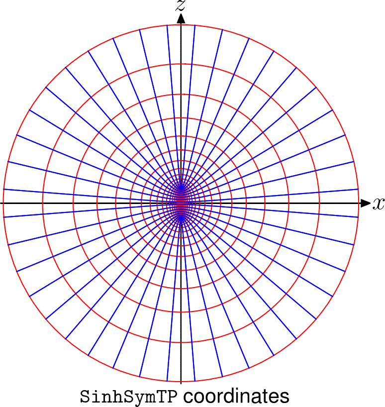
Figure 1: Curves of constant $\mathtt{x_{1}}$ (red) and constant $\mathtt{x_{2}}$ (blue) using a cell-centered grid structure with $\mathtt{x_{3}}=0$.

As with TwoPunctures, NRPyEllipticET possesses the option to rotate the coordinate system, to situate the punctures on either the $x$-axis ($x=\pm b$) or the $z$-axis ($z=\pm b$).

For all cases considered here, the outer boundary is set to $10^{6}$ (i.e., $\mathcal{A}=10^{6}$), and the grid point spacing parameter $w$ is set to $0.07$. We set $b$ so that the foci match the punctures’ positions and, when interpolating the ID to the Einstein Toolkit grids, we adjust the origin of the coordinate system to coincide with the center of mass of the punctures, as is conventional.

III.2 Wavespeed

To propagate the hyperbolic system of equations forward in (pseudo)time from the chosen initial conditions, we make use of NRPy+’s method of lines implementation. Specifically we choose the explicit fourth-order Runge-Kutta (RK4) method. As this is an explicit method, and we use three dimensions in space, the steps in time $\Delta t$ are constrained by the CFL inequality:

$$\frac{c\Delta t}{\Delta s_{\rm min}}\leq\mathcal{C}_{0}\,,$$ (34)

where $c$ is the local wavespeed, and $\mathcal{C}_{0}$ is the CFL factor, which depends on the explicit time stepping method and the dimensionality of the problem. Empirically we find that $\mathcal{C}_{0}=0.7$ ensures both stability and large time steps for both 2D and 3D cases presented in this paper, with one exception: when the 3D case is pushed to very high resolution. In the single highest-resolution 3D case in this work, we find $\mathcal{C}_{0}$ must be lowered to $0.55$ for stability.

Further, $\Delta s_{\rm min}$ is the minimum proper distance between neighboring points in our curvilinear coordinate system:

$$\Delta s_{\rm min}=\min\left(h_{1}\mathtt{\Delta x_{1}},\,h_{2}\mathtt{\Delta x_{2}},\,h_{3}\mathtt{\Delta x_{3}}\right)\,,$$ (35)

where $h_{i}$ and $\mathtt{\Delta x_{i}}$ are the $i$-th scale factor and grid spacing of the flat space metric, respectively.

The global relaxation time step $\Delta t_{\rm glob}$ is given by the minimum value of $\Delta s_{\rm min}$ on our numerical grid. As we adopt prolate spheroidal-like coordinates, the global $\Delta s_{\rm min}$ occurs precisely at the foci of the coordinate system. At this point, for simplicity we set the wavespeed $c=1$. As this is merely a relaxation (as opposed to a physical) wavespeed, we increase $c$ in proportion to the local $\Delta s_{\rm min}$, which grows exponentially away from the foci. In this way we maintain satisfaction of the CFL inequality while greatly improving the performance of the relaxation method. Details and implications of our implementation are described in Appendix B.

III.3 Choice of damping parameter $\eta$

Sweeping through values of $\eta$ in early tests of our code (using different grid parameters than those adopted here), we found that setting $\eta=12.5/M$ was optimal for minimizing the time to convergence of the relaxation scheme. After completing the tests, we later found that this is value of $\eta$ is not optimal for the grids and resolutions we chosen in this work. As a result, our core benchmark in Sec. IV.2 below, comparing the performance of NRPyElliptic with TwoPunctures is slower by roughly a factor of 2 as compared to the optimum $\eta$ for that grid choice, which would be closer to $\eta=18/M$. We note that this sub-optimal choice does not influence our relaxed solution, as every choice of $\eta$ that leads to a stable evolution yields that same relaxed solution.

To find the optimal value of $\eta$, we perform a linear sweep through possible values in a range $\eta=1$ through 20, in intervals of $0.25$ (recall $\eta$ has units of inverse mass, $1/M$, and here when quoting values of $\eta$ we always choose $M=1$). In the steady-state regime, the $L^{2}$-norm of the relative error, $E$ (see Sec. IV for details), becomes constant. Therefore once we have chosen a trial value of $\eta$, we perform the relaxation until $|dE/dt|<\delta$ for $n$ consecutive iterations, where $\delta\sim 10^{-4}{-}10^{-6}$ and $n\sim 10{-}100$. I.e., we relax until the $L^{2}$-norm of the relative error has reached its minimum, constant value. The optimum value of $\eta$ is that value that results in the fewest relaxation iterations before the $L^{2}$-norm of the relative error has plateaued.

As $\eta$ has units of $1/t$, it is natural to inquire whether the optimum damping parameter, $\eta_{\rm optimum}$, is inversely proportional to the relaxation-wave-crossing time, $T_{\rm RC}$. We applied the aforementioned optimum $\eta$ search to a variety of grids, each with its own $T_{\rm RC}$ (in the range $T_{\rm RC}\in(0.24,0.99)$), finding that the optimum $\eta$ obeys the following power law:

$$M\eta_{\rm optimum}\approx\frac{6.9}{(T_{\rm RC}/M)^{0.79}}-0.7.$$ (36)

IV Results

Validation of NRPyElliptic is performed in two stages. First we generate initial data (ID) for a given physical scenario with the widely used TwoPunctures [31] code, increasing resolution on the TwoPunctures grids until roundoff error dominates its numerical solution of Eq. (18), $u$. We refer to this high-resolution result as the trusted solution. Second we generate the same ID with NRPyElliptic, and demonstrate that its results approach the trusted solution at the expected convergence rate.

We repeat this procedure twice: first for an axisymmetric case of two equal-mass BHs with spin vectors collinear with their separation vector, and second for a full 3D case involving a GW150914-like unequal-mass, quasi-circular, spinning BBH system. To demonstrate the fidelity of the latter case, we first generate NRPyElliptic and TwoPunctures ID at similar levels of accuracy. Then, using the Einstein Toolkit [46, 47, 48] we evolve the ID through inspiral, merger, and ringdown, and compare the results. Finally we note that $M=M_{+}+M_{-}$ is defined as the sum of individual ADM masses of the punctures (Eq. (83) of Ref. [31]).

IV.1 Axisymmetric initial data

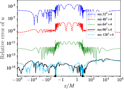
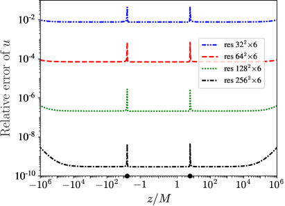
Figure 2: Calibration of TwoPunctures and NRPyElliptic solutions, axisymmetric ID study. Top: Relative errors between a super-high resolution ($196^{2}{\times}4$) and lower-resolution results from the TwoPunctures code. Bottom: Calibration of NRPyElliptic solutions at various resolutions ($\mathtt{N_{1}}{\times}\mathtt{N_{2}}{\times}6$), comparing against the trusted solution (i.e., the TwoPunctures result at $96^{2}{\times}4$ resolution). The horizontal axis is logarithmic in the range $|z|>1$ and linear otherwise. Further, the black dots on the horizontal axes denote the puncture BH positions (also the locations of the coordinate foci). TwoPunctures data were rotated so that the punctures and the foci lie on the $z$ axis.

In this test, we generate initial data (ID) for a scenario symmetric about the $z$-axis: two equal-mass punctures at rest, with spin components $\vec{S}_{\pm}=\pm 0.4M_{\pm}^{2}\hat{z}$ and initial positions $z_{\pm}=\pm 6M$.

We start by constructing the trusted solution $u$, against which we will compare results from NRPyElliptic. The trusted solution is generated by increasing the resolution of the TwoPunctures numerical grids until roundoff errors dominate. As we adopt double-precision arithmetic, this occurs when relative errors reach levels of roughly $10^{-14}$. The top panel of Fig. 2 indicates that this occurs at a TwoPunctures grid resolution of $N_{A}\times N_{B}\times N_{\phi}=96^{2}\times 4$.

After obtaining this $96^{2}\times 4$ trusted solution, we next compare it against NRPyElliptic at various resolutions in the bottom panel of the figure. To allow for a point-wise comparison, we use the spectral interpolator in TwoPunctures [57] to evaluate the TwoPunctures solution at every point on our grid. Notice that the numerical errors drop by roughly $2^{9}$ each time the resolution is doubled, indicating that numerical convergence is dominated by our choice of $10^{\rm th}$-order finite-difference (FD) stencils. That perfect $10^{\rm th}$-order convergence is not obtained is unsurprising, as our outer boundary condition is approximate and implements its own $6^{\rm th}$-order FD stencils.

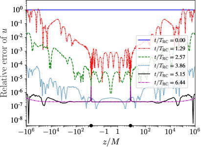
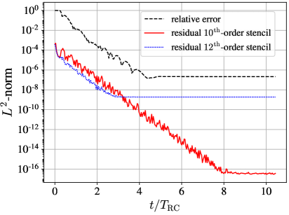
Figure 3: Axisymmetric ID study. Top: Snapshots of the relative error between the NRPyElliptic solution at $128^{2}{\times 4}$ resolution and the trusted solution at different times. TwoPunctures data were rotated so that the punctures and the foci lie on the $z$ axis. Bottom: Black dashed curve: $L^{2}$-norm of the same relative error as the top panel, computed within a sphere with radius $r=100M$ and as a function of time. Blue (dotted) and red (solid) curves: $L^{2}$-norms of residuals (second term in Eq. 18) computed within the same sphere at two different finite-difference orders as a function of time.

The exponential convergence in time of the hyperbolic relaxation method can be readily seen in Fig. 3. In the top panel snapshots of the relative error at resolution $128^{2}{\times}6$ are shown as a function of relaxation-wave-crossing times, or RCTs (i.e., the time required for a relaxation wave to cross the numerical domain; see Appendix B). During the first RCT, the errors decrease (increase) in the region near (away from) the punctures and subsequently drop exponentially in time. Numerical errors are consistently smaller in the region near the origin due to the extreme grid focusing there. Notice that after ${\sim}4$ RCTs the relative errors between the punctures have already reached the same order of magnitude as that of the fully relaxed solution, and the remaining relaxation time (40% of the total) is spent decreasing the relative errors away from the punctures.

Coincident with the exponential relaxation along the $z$-axis, the $L^{2}$-norm of both the relative errors and residual (second term in the left-hand side of Eq. 18), computed inside a sphere of radius $100M$ around the origin (situated at the center of mass), displays a steady exponential drop, as illustrated in the bottom panel of Fig. 3. We find that when the FD order for computing the residual matches the one used by the relaxation algorithm, the $L^{2}$-norm of the residual continues to drop even after the steady state has been reached, until roundoff errors dominate this measure of residual. This indicates that the residual has become overspecialized to the approximation adopted for the FD operators. To ameliorate this, we also compute the residual using 12^th-order stencils, finding this measure of the residual to have more consistent behavior with the true error (i.e., the relative error against the trusted solution). We repeated this analysis at 8^th and 14^th finite-differencing order and found the same qualitative behavior as 12^th order.

IV.2 Full 3D initial data

The second test consists of two punctures with mass ratio $q=36/29$, in a quasicircular orbit emulating the GW150914 event [58]. The punctures are located at $z=\pm 5M$, with spin components $\vec{S}_{+}=0.31M_{+}^{2}\hat{y}$ and $\vec{S}_{-}=-0.46M_{-}^{2}\hat{y}$.

The validation procedure for both TwoPunctures and NRPyElliptic follows the prescription used in the axisymmetric case. Since the full-3D system does not posses axial symmetry, the number of grid points along the azimuthal direction is no longer minimal. As indicated in the top panel of Fig. 4, the trusted TwoPunctures solution has resolution $96^{2}{\times}16$, and we found that using $N_{\phi}>16$ does not lower the relative errors further. In NRPyElliptic (bottom panel of Fig. 4), the optimal resolution in the azimuthal direction was also found to be $\mathtt{N_{3}}=16$, except for when the highest resolution ($256^{2}\times 24$) was chosen. We find this solution to have smaller relative errors when compared to the $256^{2}\times 16$ resolution data (not shown), and requires a lower CFL-factor of $\mathcal{C}_{0}=0.55$ for numerical stability. With truncation errors dominated by sampling in the $\mathtt{x_{1}}$ and $\mathtt{x_{2}}$ directions, we find roughly $9^{\rm th}$-order convergence for this case as well.

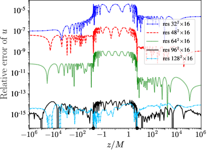
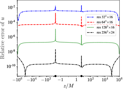
Figure 4: Same as Fig. 2, but for GW150914-like, full-3D BBH initial data.

As expected, the relaxation to the steady state has exponential convergence in (pseudo)time as depicted in both panels of Fig. 5. Although the relaxation requires a larger number of RCTs in the full-3D case, its qualitative behavior is the same.

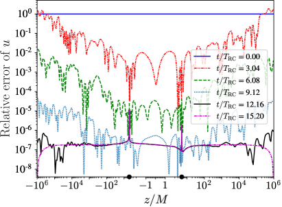
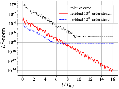
Figure 5: Same as Fig. 3, but for GW150914-like, full-3D BBH initial data, with NRPyElliptic resolution of $128^{2}{\times}16$.

Next, to demonstrate the fidelity of full-3D initial data generated by NRPyElliptic, we first generate ID for the GW150914-like BBH scenario using both NRPyElliptic and TwoPunctures. These ID are chosen to be of comparable quality, as shown in Fig. 6. Precise numerical parameters for the ID exactly follow the GW150914 Einstein Toolkit gallery example [59, 46, 60, 61, 62, 31, 63, 64, 65, 66, 67], for which complete results are freely available online. Notably the TwoPunctures code required slightly less than a minute to generate the ID (we input the bare masses directly), while NRPyElliptic required about 10 minutes, for a difference in performance of ${\approx}12$x.

After generation, the ID from both codes are interpolated onto the evolution grids, which consist of a set of Carpet [61]-managed Cartesian AMR patches in the strong field region, with resolution around the punctures of ${\approx}M/52$. These AMR patches are surrounded by a Llama [62]-managed cubed spheres grid in the weak-field region. When interpolating the ID onto these grids, TwoPunctures adopts a high-accuracy spectral interpolator (see e.g., [57]), and NRPyElliptic uses the third-order Hermite polynomial interpolator from the AEILocalInterp thorn. As our choice of Hermite interpolation order results in far less accuracy, it introduces error to the Hamiltonian constraint violation at time $t=0$ on the orbital plane, as shown in the left panel of Fig. 7.

We then evolve these ID forward in time using the McLachlan BSSN thorn [65]. Notice that after the first orbital period the Hamiltonian constraint violations on the orbital plane are essentially identical (right panel of Fig. 7), indicating that numerical errors associated with the evolution quickly dominate ID errors.

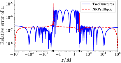
Figure 6: Initial data quality of the GW150914-like BBH 3D scenario evolved with the Einstein Toolkit, showing the relative error of $u$ against the trusted TwoPunctures solution. Here TwoPunctures and NRPyElliptic ID used resolutions of $38^{2}\times 16$ and $128^{2}\times 16$ respectively. Note that TwoPunctures data were rotated so that the punctures are positioned on the $z$ axis.

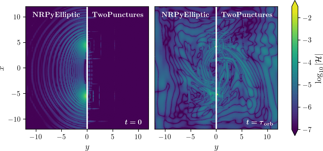
Figure 7: Hamiltonian constraint violation $\log_{10}\left|\mathcal{H}\right|$, as defined in Eq. (4), in orbital plane after interpolation to AMR grids at $t=0$ (left) and after one orbit (right). Note that NRPyElliptic data were rotated so that the punctures are positioned on the $x$ axis.

Figure 8: Simulation results with ID by TwoPunctures (solid, blue) and NRPyElliptic (dashed, orange-red). Left: Dominant mode ($\ell=2$, $m=2$) of the Weyl scalar $\psi_{4}$ at extraction radius $r_{\rm ext}=500M$. Right: Trajectory of the less-massive BH.

Finally, to demonstrate that NRPyElliptic’s 3D data are of sufficiently high fidelity, we demonstrate that when they are evolved forward in time the results are indistinguishable from an evolution of TwoPunctures ID at comparable initial accuracy. For instance in Fig. 8 we show the trajectory of the less-massive BH and the dominant mode ($\ell=2$, $m=2$) of the Weyl scalar $\psi_{4}$, for both evolutions. We find that quantities extracted from the evolution of NRPyElliptic ID to be in excellent agreement with results from evolution of ID from the trusted TwoPunctures code. Although not shown, the trajectory of the more-massive BH for both simulations are also visually indistinguishable, as are other, higher-order $\psi_{4}$ modes.

V Conclusions and Future Work

NRPyElliptic is an extensible ID code for numerical relativity that recasts non-linear elliptic PDEs as covariant, hyperbolic PDEs. To this end it adopts the hyperbolic relaxation method of [39], in which the (pseudo)time evolution of the hyperbolic PDEs exponentially relaxes to a steady state consistent with the solution to the elliptic problem. That standard hyperbolic methods are used to solve the elliptic problem is beneficial, as consumers of numerical relativity ID generally already have expertise in solving hyperbolic PDEs. Thus the learning curve is significantly lowered for core users of NRPyElliptic, enabling them to build on existing expertise to modify and extend the solver.

NRPyElliptic leverages NRPy+’s reference metric infrastructure to solve the hyperbolic/elliptic PDEs in a wide variety of Cartesian-like, spherical-like, cylindrical-like, and bispherical-like coordinate systems. As its first application, in NRPyElliptic we solve a nonlinear elliptic PDE to set up two-puncture ID for numerical relativity. Similar to the TwoPunctures [31] code, NRPyElliptic solves the elliptic PDE for the Hamiltonian constraint in a prolate spheroidal-like coordinate system. But unlike the one-parameter coordinate system used in prolate-spheroidal coordinates or TwoPunctures coordinates, NRPyElliptic adopts NRPy+’s SinhSymTP three-parameter coordinate system, providing greater flexibility in setting up the numerical grid.

As the SinhSymTP numerical grid is not compactified, finite-radius boundary conditions must be applied. To address this, a new radiation boundary condition algorithm within NRPy+ has been developed, which is based on the widely used NewRad radiation boundary condition driver within the Einstein Toolkit. While NewRad implements a second-order approach, NRPyElliptic extends to fourth and sixth finite difference orders as well. This high-order boundary condition meshes well with the high (tenth) order finite-difference representation of the elliptic operators adopted in NRPyElliptic.

To greatly accelerate the relaxation, we set the wavespeed of the hyperbolic PDEs to grow in proportion to the grid spacing. As the SinhSymTP grid spacing grows exponentially with distance from the central region of the coordinate system, so does the relaxation wavespeed. Thus this approach is many orders of magnitude faster than the traditional, constant-wavespeed choice, in fact making it fast enough to set up high-quality, full-3D BBH ID for numerical relativity.

Although NRPyElliptic currently requires only a tiny fraction of the total runtime of a typical NR BBH merger calculation, it is roughly 12x slower than TwoPunctures when setting up the full-3D BBH ID in this work. Efforts in the immediate future will in part focus on improving this performance. To this end, a couple of ideas come to mind. First, all ID generated in this work used the trivial ($u=v=0$) initial guess. We plan to explore whether relaxations at lower-resolutions might be used to provide a superior initial guess on finer grids, in which convergence is accelerated.

Second, due to the CFL condition, the speed of NRPyElliptic is proportional to the smallest grid spacing, which occurs at the foci of our SinhSymTP coordinate system. Typical grid spacings at the foci are ${\sim}10^{-4}M$ due to extreme grid focusing there, which in turn are ${\sim}1/100$ those typically used in (near-equal-mass) binary puncture evolutions, indicating that a significant speed-up may be possible if superior grid structures are used.

To this end, we plan to adopt the same seven-grid bispheres grids infrastructure adopted by the NRPy+-based BlackHoles@Home [68] project. As illustrated in Fig. 9, seven-grid BiSpheres consists of seven overlapping spherical-like and Cartesian-like grids. This approach places Cartesian-like AMR grid patches over regions where the spherical-like grids would otherwise experience extreme grid focusing ($r\to 0$), constraining the smallest grid spacings in the strong-field region to ${\approx}M/200$. Thus with such grids, accounting for needed inter-grid interpolations, we might expect roughly a ${\sim}10$x increase in speed—making NRPyElliptic comparable in performance to TwoPunctures for near-equal-mass-ratio systems—all while maintaining excellent resolution in the strong-field region. Further, the Cartesian-like AMR patches on these grids are centered precisely at the locations of the compact objects, making them efficiently tunable to higher mass ratios, unlike SinhSymTP or other prolate spheroidal-like coordinates mentioned in this work. Extending NRPyElliptic to higher mass ratios in this way, as well as to other types of NR ID, will be explored in forthcoming papers.

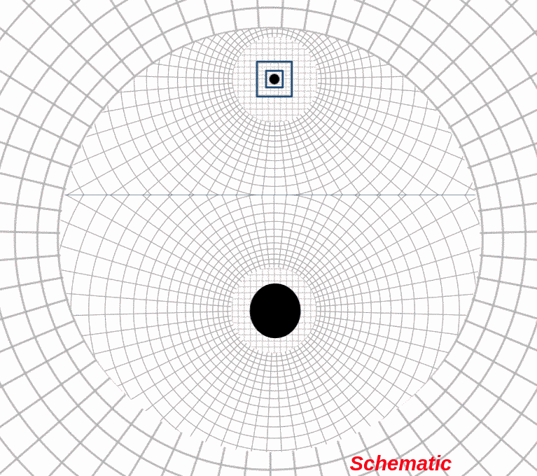
Figure 9: Schematic of seven-grid BiSpheres numerical meshes used for BlackHoles@Home ${\sim}$6:1 mass-ratio BBH simulations during the long inspiral phase. BHs are represented as black dots.

Appendix A Sommerfeld Boundary Conditions

Sommerfeld boundary conditions (BCs)—also referred to as radiation or transparent boundary conditions—aim to enable outgoing wave fronts to pass through the boundaries of a domain with minimal reflection. Sommerfeld BCs typically assume that for large values of $r$ any given field $f=f(t,r)$ behaves as an outgoing spherical wave, with an asymptotic value $f_{0}$ as $r\to\infty$. Following NewRad [54], our ansatz for $f(t,r)$ on the boundary takes the form

$$f=f_{0}+\frac{w(r-ct)}{r}+\frac{C}{r^{n}}\,,$$ (37)

where $w(r-ct)/r$ represents an outgoing wave that solves the wave equation in spherical symmetry, and $C$ is a constant. The $1/r^{n}$ correction term encapsulates higher-order corrections with $n>1$ fall-off.

We follow the hyperbolic relaxation method of [39] and NewRad, and apply Sommerfeld boundary conditions not to $f$ directly, but to $\partial_{t}f$:

$$\partial_{t}f=-c\frac{w^{\prime}(r-ct)}{r}\,.$$ (38)

To better understand the $w^{\prime}(r-ct)$ term, we compute the radial partial derivative of $f$ as well:

$$\partial_{r}f=\frac{w^{\prime}(r-ct)}{r}-\frac{w(r-ct)}{r^{2}}-n\frac{C}{r^{n+1}}\,.$$ (39)

Solving Eq. (39) for $w^{\prime}(r-ct)$ and substituting into Eq. (38) yields

$$\partial_{t}f=-c\left[\partial_{r}f+\frac{w(r-ct)}{r^{2}}+n\frac{C}{r^{n+1}}\right]\,.$$ (40)

To take care of the (as-yet) unknown $w(r-ct)/r^{2}$ term, notice that our ansatz Eq. (37) implies

$$\frac{w(r-ct)}{r^{2}}=\frac{f-f_{0}}{r}-\frac{C}{r^{n+1}}\,,$$ (41)

which when inserted into Eq. (40) yields

$$\partial_{t}f=-c\biggl{[}\partial_{r}f+\frac{f-f_{0}}{r}\biggr{]}+\frac{k}{r^{n+1}}\,,$$ (42)

where $k=-cC(n-1)$ is just another constant. Thus we have derived the desired boundary condition

$$\partial_{t}f=-\frac{c}{r}\bigl{[}r\partial_{r}f+(f-f_{0})\bigr{]}+\frac{k}{r^{n+1}}\,.$$ (43)

To generalize Eq. (43) to arbitrary curvilinear coordinate systems $x^{i}_{\rm Curv}$, we make use of the chain rule

$$\frac{\partial f\bigl{(}x^{i}_{\rm Curv}\bigr{)}}{\partial r}=\biggl{(}\frac{\partial x^{i}_{\rm Curv}}{\partial r}\biggr{)}\biggl{(}\frac{\partial f}{\partial x^{i}_{\rm Curv}}\biggr{)}\,,$$ (44)

which can be plugged into Eq. (43) to give us Eq. (29)

$$\partial_{t}f=-\frac{c}{r}\left[r\frac{\partial x^{i}_{\rm Curv}}{\partial r}\frac{\partial f}{\partial x^{i}_{\rm Curv}}+(f-f_{0})\right]+\frac{k}{r^{n+1}}\,.$$ (45)

Returning to the original ansatz (Eq. 37), we would generally expect the lowest-order correction to be one order higher than the dominant, $1/r$ falloff. As the correction term in Eq. (37) has $1/r^{n}$ falloff, we therefore set $n=2$ to obtain our final expression for imposing outgoing radiation boundary conditions any given field $f$:

$$\boxed{\partial_{t}f=-\frac{c}{r}\left[r\frac{\partial x^{i}_{\rm Curv}}{\partial r}\frac{\partial f}{\partial x^{i}_{\rm Curv}}+(f-f_{0})\right]+\frac{k}{r^{3}}}\ .$$ (46)

Regarding numerical implementation of this expression a couple of subtleties arise. First, note that $\partial x^{i}_{\rm Curv}/\partial r$ may be impossible to compute analytically, as the spherical radius $r$ is generally easy to write in terms of the curvilinear coordinates $x^{i}_{\rm Curv}$, but not its inverse $x^{i}_{\rm Curv}(r)$.

To address this, for all coordinate systems $x^{i}_{\rm Curv}$ implemented in NRPy+, the function

$$x^{i}_{\rm Sph}=\biggl{(}r(x^{i}_{\rm Curv}),\theta(x^{i}_{\rm Curv}),\phi(x^{i}_{\rm Curv})\biggr{)}\,,$$ (47)

is explicitly defined. If we define the Jacobian

$$J^{j}_{\ i}=\frac{\partial x^{j}_{\rm Sph}}{\partial x^{i}_{\rm Curv}}\,,$$ (48)

and use NRPy+ functions to invert this matrix, we obtain exact expressions for the inverse Jacobian matrix, which encodes $\partial x^{i}_{\rm Curv}/\partial x^{j}_{\rm Sph}$:

$$\bigl{(}J^{-1}\bigr{)}^{i}_{\ j}=\frac{\partial x^{i}_{\rm Curv}}{\partial x^{j}_{\rm Sph}}\,.$$ (49)

From this, we can express $\partial x^{i}_{\rm Curv}/\partial r$ exactly for any curvilinear coordinate system implemented within NRPy+.

The second subtlety lies in formulating a way to approximate $k$. If the function $f$ represented only an outgoing spherical wave, then it would exactly satisfy the advection equation

$$\biggl{[}\frac{\partial f}{\partial t}\biggr{]}_{\rm adv}\equiv-\frac{c}{r}\bigg{[}r\frac{\partial x^{i}_{\rm Curv}}{\partial r}\frac{\partial f}{\partial x^{i}_{\rm Curv}}+(f-f_{0})\bigg{]}\,,$$ (50)

which is identical to Eq. (46) but with $k=0$.

Next consider an interior point $r_{\rm int}$ directly adjacent to the outer boundary. Then, $f(r_{\rm int})$ approximately satisfies both the time evolution equation (e.g. Eq. 25), and the advection equation Eq. (50). We compute $\partial_{t}f(r_{\rm int})$ for a given field $f$ directly from evaluating the corresponding right-hand side of Eq. (21), and $[\partial_{t}f]_{\rm adv}(r_{\rm int})$ from Eq. (50). The difference of these two equations yields the departure from the expected purely outgoing wave behavior at that point $k/r_{\rm int}^{n+1}$. From this we can immediately extract $k$:

$$\boxed{k=r_{\rm int}^{3}\left(\frac{\partial f}{\partial t}-\left[\frac{\partial f}{\partial t}\right]_{\rm adv}\right)_{\rm int}}\ ,$$ (51)

where again we impose $n=2$.

Our numerical implementation of Sommerfeld BCs evaluates $\partial f/\partial x^{i}_{\rm Curv}$ in Eq. (50) using either centered or fully upwinded finite-difference derivatives as needed to ensure finite-difference stencils do not reach out of bounds. Unlike NewRad, which only implements second-order finite-difference derivatives for $\partial f/\partial x^{i}_{\rm Curv}$, our implementation supports second, fourth, and sixth-order finite differences.

We validated this Sommerfeld boundary condition algorithm against NewRad for the case of a scalar wave propagating across a 3D Cartesian grid, choosing second-order finite-difference derivatives in our algorithm. We achieved roundoff-level agreement for the wave propagating toward each of the individual faces.

Appendix B Spatially-dependent wavespeed and relaxation-wave-crossing time

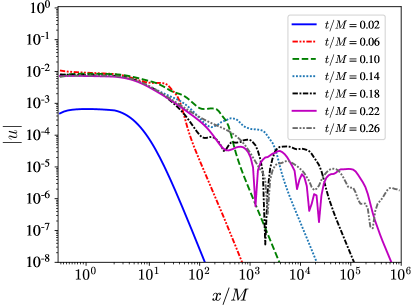
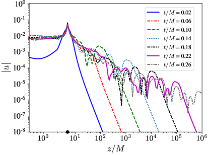
Figure 10: Top: Propagation of $u$ along gridpoints closest to the $x$-axis during the first relaxation-wave-crossing time for the 3D ID. Bottom: Same as top panel, except for gridpoints closest to the $z$-axis.

At every point in the domain we compute the smallest proper distance between neighboring points, $\Delta S_{\rm{min}}$, and define a local wavespeed that is proportional to the grid spacing as

$$c(\vec{x})=\mathcal{C}_{0}\frac{\Delta S_{\rm{}min}(\vec{x})}{\Delta t}\,,$$ (52)

where $\Delta t$ is the time step used by the time integrator, and $\mathcal{C}_{0}$ is the CFL factor.

For the sake of readability, we repeat here the relationship between SinhSymTP coordinates and Cartesian coordinates,

$$x =\tilde{r}\sin(\mathtt{x_{2}})\cos(\mathtt{x_{3}})\,,$$

$$y =\tilde{r}\sin(\mathtt{x_{2}})\sin(\mathtt{x_{3}})\,,$$ (53)

$$z =\left(\tilde{r}^{2}+b^{2}\right)^{1/2}\cos(\mathtt{x_{2}})\,.$$

To establish the time scales associated with the propagation of relaxation waves, we calculate the relaxation-wave-crossing time along the $x$-axis—$\left(\mathtt{x_{2}},\mathtt{x_{3}}\right)=\left(\pi/2,0\right)$ in Eqs. (B)—and the $z$-axis. NRPyElliptic adopts topologically Cartesian, cell-centered grids with inter-cell spacing of $\mathtt{\Delta x_{1}}$, $\mathtt{\Delta x_{2}}$, and $\mathtt{\Delta x_{3}}$ in the $\mathtt{x_{1}}$, $\mathtt{x_{2}}$, and $\mathtt{x_{3}}$-directions, respectively. Because of this, the closest points to the $x$-axis are obtained by setting $\mathtt{x_{2}}=(\pi+\mathtt{\Delta x_{2}})/2$ and $\mathtt{x_{3}}=\mathtt{\Delta x_{3}}/2$. Likewise, the closest points to the $z$-axis are given by setting $\mathtt{x_{2}}=\mathtt{\Delta x_{2}}/2$ and $\mathtt{x_{3}}$ to any fixed value. The relaxation-wave crossing time along the $x$-axis is given by

$$T_{\rm{RC}}^{(x)} =\int\frac{dx}{c(x)}\ =\int_{\mathtt{x_{1}}=0}^{1}\frac{f(\mathtt{x_{1}})d\mathtt{x_{1}}}{c^{(x)}(\mathtt{x_{1}})}\,,$$ (54)

where

$$f(\mathtt{x_{1}})=\partial_{\mathtt{x_{1}}}x(\mathtt{x_{1}},\mathtt{x_{2}},\mathtt{x_{3}})\Big{|}_{\mathtt{x_{2}}=(\pi+\mathtt{\Delta x_{2}})/2,\mathtt{x_{3}}=\mathtt{\Delta x_{3}}/2}\,,$$ (55)

and $c^{(x)}$ is the wavespeed along the $x$-axis. For the choice of grid parameters described in Sec. III, the smallest grid spacing along the $x$-axis is given by the proper distance in the direction of the $\mathtt{x_{2}}$ coordinate, so that

$$c^{(x)}(\mathtt{x_{1}})=\mathcal{C}_{0}\frac{\Delta S^{(2)}(\mathtt{x_{1}})}{\Delta t}\ =\frac{\mathcal{C}_{0}\mathtt{\Delta x_{2}}}{\Delta t}h^{(2)}(\mathtt{x_{1}})\,,$$ (56)

where $h^{(2)}(\mathtt{x_{1}})=\sqrt{\tilde{r}^{2}(\mathtt{x_{1}})+b^{2}\cos^{2}(\mathtt{\Delta x_{2}}/2)}$ is the scale factor. Substituting Eq. (56) in Eq. (54) and integrating yields

$$T_{\rm{RC}}^{(x)} = \frac{\Delta t}{\mathcal{C}_{0}\mathtt{\Delta x_{2}}}\ \operatorname{arctanh}\left(\frac{\mathcal{A}}{\sqrt{\mathcal{A}^{2}+b^{2}\cos^{2}(\mathtt{\Delta x_{2}}/2)}}\right)$$ (57)

$$\times\sin(\mathtt{\Delta x_{2}}/2)\cos(\mathtt{\Delta x_{3}}/2)\,.$$

Similarly, the wavespeed along the $z$-axis is given by

$$c^{(z)}(\mathtt{x_{1}})=\mathcal{C}_{0}\frac{\Delta S^{(3)}(\mathtt{x_{1}})}{\Delta t}\ =\frac{\mathcal{C}_{0}\mathtt{\Delta x_{3}}}{\Delta t}h^{(3)}(\mathtt{x_{1}})\,,$$ (58)

where $h^{(3)}(\mathtt{x_{1}})=\tilde{r}(\mathtt{x_{1}})\sin(\mathtt{\Delta x_{2}}/2)$ is the scale factor in the direction of $\mathtt{x_{3}}$. Thus, the relaxation-wave-crossing time along the $z$-axis can be computed as

$$T_{\rm{RC}}^{(z)} =\int\frac{dz}{c(z)}\ =\int_{\mathtt{x_{1}}=0}^{1}\frac{g(\mathtt{x_{1}})d\mathtt{x_{1}}}{c^{(z)}(\mathtt{x_{1}})}$$

$$=\frac{\Delta t}{\mathcal{C}_{0}\mathtt{\Delta x_{3}}}\ \operatorname{arctanh}\left(\frac{\mathcal{A}}{\sqrt{\mathcal{A}^{2}+b^{2}}}\right)\cot(\mathtt{\Delta x_{2}}/2)\,,$$ (59)

where we used

$$g(\mathtt{x_{1}})=\partial_{\mathtt{x_{1}}}z(\mathtt{x_{1}},\mathtt{x_{2}},\mathtt{x_{3}})\Big{|}_{\mathtt{x_{2}}=\mathtt{\Delta x_{2}}/2}\,.$$ (60)

Plugging in the values of the grid parameters $\mathcal{A}$, $w$, and step sizes, we find $T_{\rm{RC}}^{(x)}=0.248M$ ($0.574M$) and $T_{\rm{RC}}^{(z)}=1.28M$ ($1.26M$) for full-3D (axisymmetric) ID.

From Eq. (58) we find that for fixed values of $\mathtt{x_{1}}$ and small angles $\mathtt{x_{2}}$ the wavespeed along the $z$-axis behaves as

$$c^{(z)}\sim\tilde{r}(\mathtt{x_{1}})\,\mathtt{x_{2}}\,\mathtt{\Delta x_{3}}\,.$$ (61)

Our cell-centered grid has $\mathtt{x_{2}}_{\mathtt{i_{2}}}=(\mathtt{i_{2}}+1/2)\mathtt{\Delta x_{2}}$ with $\mathtt{i_{2}}=0,1,2,\ldots,\mathtt{N_{2}}$, and thus the wavespeed quickly increases as we move away from the axis. Such rapidly-moving signals slightly off the $z$-axis are not considered in our analytic estimates, yet influence the RCT so that in our full-3D simulations we observe the same value of $T_{\rm RC}\approx 0.25M\approx T_{\rm RC}^{(x)}$ along both axes, as shown in Fig. 10. Thus we use $T_{\rm RC}=T_{\rm RC}^{(x)}$ in all figures.

References

- Abbott et al. [2021] R. Abbott et al. (LIGO Scientific, VIRGO), Gwtc-2.1: Deep extended catalog of compact binary coalescences observed by ligo and virgo during the first half of the third observing run, arXiv e-prints (2021), arXiv:2108.01045 [gr-qc] .
- Nakamura et al. [1987] T. Nakamura, K.-I. Oohara, and Y. Kojima, General relativistic collapse to black holes and gravitational waves from black holes, Prog. Theor. Phys. Suppl. 90, 1 (1987).
- Shibata and Nakamura [1995] M. Shibata and T. Nakamura, Evolution of three-dimensional gravitational waves: Harmonic slicing case, Phys. Rev. D 52, 5428 (1995).
- Baumgarte and Shapiro [1999] T. W. Baumgarte and S. L. Shapiro, On the numerical integration of Einstein’s field equations, Phys. Rev. D 59, 024007 (1999), arXiv:gr-qc/9810065 .
- Pretorius [2005] F. Pretorius, Numerical relativity using a generalized harmonic decomposition, Class. Quant. Grav. 22, 425 (2005), arXiv:gr-qc/0407110 .
- Bona et al. [2003] C. Bona, T. Ledvinka, C. Palenzuela, and M. Zacek, General covariant evolution formalism for numerical relativity, Phys. Rev. D 67, 104005 (2003), arXiv:gr-qc/0302083 .
- Bernuzzi and Hilditch [2010] S. Bernuzzi and D. Hilditch, Constraint violation in free evolution schemes: Comparing BSSNOK with a conformal decomposition of Z4, Phys. Rev. D 81, 084003 (2010), arXiv:0912.2920 [gr-qc] .
- Alic et al. [2012] D. Alic, C. Bona-Casas, C. Bona, L. Rezzolla, and C. Palenzuela, Conformal and covariant formulation of the Z4 system with constraint-violation damping, Phys. Rev. D 85, 064040 (2012), arXiv:1106.2254 [gr-qc] .
- Alic et al. [2013] D. Alic, W. Kastaun, and L. Rezzolla, Constraint damping of the conformal and covariant formulation of the Z4 system in simulations of binary neutron stars, Phys. Rev. D 88, 064049 (2013), arXiv:1307.7391 [gr-qc] .
- Sanchis-Gual et al. [2014] N. Sanchis-Gual, P. J. Montero, J. A. Font, E. Müller, and T. W. Baumgarte, Fully covariant and conformal formulation of the Z4 system in a reference-metric approach: comparison with the BSSN formulation in spherical symmetry, Phys. Rev. D 89, 104033 (2014), arXiv:1403.3653 [gr-qc] .
- Knapp et al. [2002] A. M. Knapp, E. J. Walker, and T. W. Baumgarte, Illustrating stability properties of numerical relativity in electrodynamics, Phys. Rev. D 65, 064031 (2002), arXiv:gr-qc/0201051 .
- Cook [2000] G. B. Cook, Initial data for numerical relativity, Living Rev. Rel. 3, 5 (2000), arXiv:gr-qc/0007085 .
- Pfeiffer [2005] H. P. Pfeiffer, The initial value problem in numerical relativity, Journal of Hyperbolic Differential Equations 02, 497 (2005), https://doi.org/10.1142/S0219891605000518 .
- Tichy [2016] W. Tichy, The initial value problem as it relates to numerical relativity, Reports on Progress in Physics 80, 026901 (2016).
- Gourgoulhon [2007] E. Gourgoulhon, Construction of initial data for 3+1 numerical relativity, J. Phys. Conf. Ser. 91, 012001 (2007), arXiv:0704.0149 [gr-qc] .
- Tsokaros and Uryū [2007] A. A. Tsokaros and K. Uryū, Numerical method for binary black hole/neutron star initial data: Code test, Phys. Rev. D 75, 044026 (2007), arXiv:gr-qc/0703030 [gr-qc] .
- Uryū et al. [2009] K. Uryū, F. Limousin, J. L. Friedman, E. Gourgoulhon, and M. Shibata, Nonconformally flat initial data for binary compact objects, Phys. Rev. D 80, 124004 (2009), arXiv:0908.0579 [gr-qc] .
- Tsokaros et al. [2015] A. Tsokaros, K. Uryū, and L. Rezzolla, New code for quasiequilibrium initial data of binary neutron stars: Corotating, irrotational, and slowly spinning systems, Phys. Rev. D 91, 104030 (2015), arXiv:1502.05674 [gr-qc] .
- Uryū and Tsokaros [2012] K. Uryū and A. Tsokaros, New code for equilibriums and quasiequilibrium initial data of compact objects, Phys. Rev. D 85, 064014 (2012), arXiv:1108.3065 [gr-qc] .
- East et al. [2012] W. E. East, F. M. Ramazanoǧlu, and F. Pretorius, Conformal thin-sandwich solver for generic initial data, Phys. Rev. D 86, 104053 (2012), arXiv:1208.3473 [gr-qc] .
- Moldenhauer et al. [2014] N. Moldenhauer, C. M. Markakis, N. K. Johnson-McDaniel, W. Tichy, and B. Brügmann, Initial data for binary neutron stars with adjustable eccentricity, Phys. Rev. D 90, 084043 (2014), arXiv:1408.4136 [gr-qc] .
- Grandclément [2006] P. Grandclément, Accurate and realistic initial data for black hole neutron star binaries, Phys. Rev. D 74, 124002 (2006), arXiv:gr-qc/0609044 [gr-qc] .
- Gourgoulhon et al. [2001] E. Gourgoulhon, P. Grandclement, K. Taniguchi, J.-A. Marck, and S. Bonazzola, Quasiequilibrium sequences of synchronized and irrotational binary neutron stars in general relativity: 1. Method and tests, Phys. Rev. D 63, 064029 (2001), arXiv:gr-qc/0007028 .
- Pfeiffer et al. [2003] H. P. Pfeiffer, L. E. Kidder, M. A. Scheel, and S. A. Teukolsky, A multidomain spectral method for solving elliptic equations, Computer Physics Communications 152, 253 (2003), arXiv:gr-qc/0202096 .
- Ossokine et al. [2015] S. Ossokine, F. Foucart, H. P. Pfeiffer, M. Boyle, and B. Szilágyi, Improvements to the construction of binary black hole initial data, Classical and Quantum Gravity 32, 245010 (2015), arXiv:1506.01689 [gr-qc] .
- Foucart et al. [2008] F. Foucart, L. E. Kidder, H. P. Pfeiffer, and S. A. Teukolsky, Initial data for black hole neutron star binaries: A flexible, high-accuracy spectral method, Phys. Rev. D 77, 124051 (2008), arXiv:0804.3787 [gr-qc] .
- Tacik et al. [2015] N. Tacik, F. Foucart, H. P. Pfeiffer, R. Haas, S. Ossokine, J. Kaplan, C. Muhlberger, M. D. Duez, L. E. Kidder, M. A. Scheel, and B. Szilágyi, Binary neutron stars with arbitrary spins in numerical relativity, Phys. Rev. D 92, 124012 (2015), arXiv:1508.06986 [gr-qc] .
- Tacik et al. [2016] N. Tacik, F. Foucart, H. P. Pfeiffer, C. Muhlberger, L. E. Kidder, M. A. Scheel, and B. Szilágyi, Initial data for black hole-neutron star binaries, with rotating stars, Classical and Quantum Gravity 33, 225012 (2016), arXiv:1607.07962 [gr-qc] .
- Taniguchi et al. [2001] K. Taniguchi, E. Gourgoulhon, and S. Bonazzola, Quasiequilibrium sequences of synchronized and irrotational binary neutron stars in general relativity. 2. Newtonian limits, Phys. Rev. D 64, 064012 (2001), arXiv:gr-qc/0103041 .
- Taniguchi and Gourgoulhon [2002] K. Taniguchi and E. Gourgoulhon, Quasiequilibrium sequences of synchronized and irrotational binary neutron stars in general relativity. 3. Identical and different mass stars with gamma = 2, Phys. Rev. D 66, 104019 (2002), arXiv:gr-qc/0207098 .
- Ansorg et al. [2004] M. Ansorg, B. Bruegmann, and W. Tichy, A Single-domain spectral method for black hole puncture data, Phys. Rev. D 70, 064011 (2004), arXiv:gr-qc/0404056 .
- Dietrich et al. [2015] T. Dietrich, N. Moldenhauer, N. K. Johnson-McDaniel, S. Bernuzzi, C. M. Markakis, B. Brügmann, and W. Tichy, Binary neutron stars with generic spin, eccentricity, mass ratio, and compactness: Quasi-equilibrium sequences and first evolutions, Phys. Rev. D 92, 124007 (2015), arXiv:1507.07100 [gr-qc] .
- Tichy et al. [2019] W. Tichy, A. Rashti, T. Dietrich, R. Dudi, and B. Brügmann, Constructing binary neutron star initial data with high spins, high compactnesses, and high mass ratios, Phys. Rev. D 100, 124046 (2019), arXiv:1910.09690 [gr-qc] .
- Grandclément [2010] P. Grandclément, KADATH: A spectral solver for theoretical physics, Journal of Computational Physics 229, 3334 (2010), arXiv:0909.1228 [gr-qc] .
- Papenfort et al. [2021] L. J. Papenfort, S. D. Tootle, P. Grandclément, E. R. Most, and L. Rezzolla, New public code for initial data of unequal-mass, spinning compact-object binaries, Phys. Rev. D 104, 024057 (2021), arXiv:2103.09911 [gr-qc] .
- Rashti et al. [2021] A. Rashti, F. M. Fabbri, B. Brügmann, S. V. Chaurasia, T. Dietrich, M. Ujevic, and W. Tichy, Elliptica: a new pseudo-spectral code for the construction of initial data, arXiv e-prints (2021), arXiv:2109.14511 [gr-qc] .
- Barreto et al. [2018] W. Barreto, P. C. M. Clemente, H. P. de Oliveira, and B. Rodriguez-Mueller, RIO: a new computational framework for accurate initial data of binary black holes, General Relativity and Gravitation 50, 71 (2018), arXiv:1803.05833 [gr-qc] .
- Vu et al. [2022] N. L. Vu et al., A scalable elliptic solver with task-based parallelism for the SpECTRE numerical relativity code, Phys. Rev. D 105, 084027 (2022), arXiv:2111.06767 [gr-qc] .
- Rüter et al. [2018] H. R. Rüter, D. Hilditch, M. Bugner, and B. Brügmann, Hyperbolic Relaxation Method for Elliptic Equations, Phys. Rev. D 98, 084044 (2018), arXiv:1708.07358 [gr-qc] .
- Meurer et al. [2017] A. Meurer, C. P. Smith, M. Paprocki, O. Čertík, S. B. Kirpichev, M. Rocklin, A. Kumar, S. Ivanov, J. K. Moore, S. Singh, et al., Sympy: symbolic computing in python, PeerJ Computer Science 3, e103 (2017).
- Ruchlin et al. [2018] I. Ruchlin, Z. B. Etienne, and T. W. Baumgarte, SENR/NRPy+: Numerical Relativity in Singular Curvilinear Coordinate Systems, Phys. Rev. D 97, 064036 (2018), arXiv:1712.07658 [gr-qc] .
- [42] NRPy+’s webpage, http://nrpyplus.net/.
- York Jr. [1999] J. W. York Jr., Conformal ‘thin-sandwich’ data for the initial-value problem of general relativity, Phys. Rev. Lett. 82, 1350 (1999), arXiv:gr-qc/9810051 .
- Lovelace et al. [2012] G. Lovelace, M. Boyle, M. A. Scheel, and B. Szilagyi, Accurate gravitational waveforms for binary-black-hole mergers with nearly extremal spins, Class. Quant. Grav. 29, 045003 (2012), arXiv:1110.2229 [gr-qc] .
- Alcubierre [2008] M. Alcubierre, Introduction to 3+1 Numerical Relativity (Oxford University Press, Oxford, U.K., 2008).
- Loffler et al. [2012] F. Loffler et al., The Einstein Toolkit: A Community Computational Infrastructure for Relativistic Astrophysics, Class. Quant. Grav. 29, 115001 (2012), arXiv:1111.3344 [gr-qc] .
- [47] Einstein toolkit home page, http:einsteintoolkit.org.
- [48] Cactus web site, http://www.cactuscode.org.
- Press et al. [1992] W. H. Press, B. P. Flannery, S. A. Teukolsky, and W. T. Vetterling, Numerical Recipes, 2nd ed. (Cambridge University Press, New York, 1992).
- Baumgarte and Shapiro [2010] T. W. Baumgarte and S. L. Shapiro, Numerical Relativity: Solving Einstein’s Equations on the Computer (Cambridge University Press, Cambridge, U.K., 2010).
- Bowen and York Jr. [1980] J. M. Bowen and J. W. York Jr., Time-asymmetric initial data for black holes and black-hole collisions, Phys. Rev. D 21, 2047 (1980).
- Brandt and Bruegmann [1997] S. Brandt and B. Bruegmann, A Simple construction of initial data for multiple black holes, Phys. Rev. Lett. 78, 3606 (1997), arXiv:gr-qc/9703066 .
- Schnetter [2010] E. Schnetter, Time Step Size Limitation Introduced by the BSSN Gamma Driver, Class. Quantum Grav. 27, 167001 (2010), arXiv:1003.0859 [gr-qc] .
- Alcubierre et al. [2003] M. Alcubierre, B. Bruegmann, P. Diener, M. Koppitz, D. Pollney, E. Seidel, and R. Takahashi, Gauge conditions for long term numerical black hole evolutions without excision, Phys. Rev. D 67, 084023 (2003), arXiv:gr-qc/0206072 .
- [55] OpenMP home page, https://www.openmp.org.
- Moon and Spencer [2012] P. Moon and D. E. Spencer, Field theory handbook: including coordinate systems, differential equations and their solutions (Springer, 2012).
- Paschalidis et al. [2013] V. Paschalidis, Z. B. Etienne, R. Gold, and S. L. Shapiro, An efficient spectral interpolation routine for the TwoPunctures code, arXiv e-prints (2013), arXiv:1304.0457 [gr-qc] .
- Abbott et al. [2016] B. P. Abbott et al. (LIGO Scientific, Virgo), Observation of Gravitational Waves from a Binary Black Hole Merger, Phys. Rev. Lett. 116, 061102 (2016), arXiv:1602.03837 [gr-qc] .
- Wardell et al. [2016] B. Wardell, I. Hinder, and E. Bentivegna, Simulation of GW150914 binary black hole merger using the Einstein Toolkit (2016).
- Pollney et al. [2011] D. Pollney, C. Reisswig, E. Schnetter, N. Dorband, and P. Diener, High accuracy binary black hole simulations with an extended wave zone, Phys. Rev. D 83, 044045 (2011), arXiv:0910.3803 [gr-qc] .
- Schnetter et al. [2004] E. Schnetter, S. H. Hawley, and I. Hawke, Evolutions in 3-D numerical relativity using fixed mesh refinement, Class. Quant. Grav. 21, 1465 (2004), arXiv:gr-qc/0310042 .
- Thornburg [2004] J. Thornburg, A Fast apparent horizon finder for three-dimensional Cartesian grids in numerical relativity, Class. Quant. Grav. 21, 743 (2004), arXiv:gr-qc/0306056 .
- Dreyer et al. [2003] O. Dreyer, B. Krishnan, D. Shoemaker, and E. Schnetter, Introduction to isolated horizons in numerical relativity, Phys. Rev. D 67, 024018 (2003), arXiv:gr-qc/0206008 .
- Goodale et al. [2003] T. Goodale, G. D. Allen, G. Lanfermann, J. Massó, T. Radke, E. Seidel, and J. Shalf, The Cactus Framework and Toolkit: Design and Applications, in Vector and Parallel Processing - VECPAR’2002, 5th International Conference, Lecture Notes in Computer Science (Springer, Berlin, 2003).
- Brown et al. [2009] J. D. Brown, P. Diener, O. Sarbach, E. Schnetter, and M. Tiglio, Turduckening black holes: An Analytical and computational study, Phys. Rev. D 79, 044023 (2009), arXiv:0809.3533 [gr-qc] .
- Husa et al. [2006] S. Husa, I. Hinder, and C. Lechner, Kranc: A Mathematica application to generate numerical codes for tensorial evolution equations, Comput. Phys. Commun. 174, 983 (2006), arXiv:gr-qc/0404023 .
- Thomas and Schnetter [2010] M. Thomas and E. Schnetter, Simulation factory: Taming application configuration and workflow on high-end resources, in Grid Computing (GRID), 2010 11th IEEE/ACM International Conference on (2010) arXiv:1008.4571 [cs.DC] .
- [68] Blackholes@home home page, http://blackholesathome.net/.