Revisiting the apparent horizon finding problem with multigrid methods

Abstract

Apparent horizon plays an important role in numerical relativity as it provides a tool to characterize the existence and properties of black holes on three-dimensional spatial slices in 3+1 numerical spacetimes. Apparent horizon finders based on different techniques have been developed. In this paper, we revisit the apparent horizon finding problem in numerical relativity using multigrid-based algorithms. We formulate the nonlinear elliptic apparent horizon equation as a linear Poisson-type equation with a nonlinear source, and solve it using a multigrid algorithm with Gauss-Seidel line relaxation. A fourth order compact finite difference scheme in spherical coordinates is derived and employed to reduce the complexity of the line relaxation operator to a tri-diagonal matrix inversion. The multigrid-based apparent horizon finder developed in this work is capable of locating apparent horizons in generic spatial hypersurfaces without any symmetries. The finder is tested with both analytic data, such as Brill-Lindquist multiple black hole data, and numerical data, including off-centered Kerr-Schild data and dynamical inspiraling binary black hole data. The obtained results are compared with those generated by the current fastest finder AHFinderDirect (Thornburg, Class. Quantum Grav. 21, 743, 2003), which is the default finder in the open source code Einstein Toolkit. Our finder performs comparatively in terms of accuracy, and starts to outperform AHFinderDirect at high angular resolutions ($\sim 1^{\circ}$) in terms of speed. Our finder is also more flexible to initial guess, as opposed to the Newton’s method used in AHFinderDirect. This suggests that the multigrid algorithm provides an alternative option for studying apparent horizons, especially when high resolutions are needed.

Keywords: apparent horizon, multigrid, compact finite differences, Poisson equations

1 Introduction

Apparent horizon has been an important concept for the numerical studies of spacetime that involve black holes. It serves as a real-time indicator of the existence of a black hole in numerical simulations, as its presence implies the presence of a surrounding event horizon [24]. The determination of apparent horizon during numerical simulations is made possible because of its local nature. This is in contrast to the teleological nature of event horizon, whose determination requires the full knowledge of the future evolution of a spacetime. Knowing the presence of an apparent horizon during simulation is important not only because it allows the estimation of the properties of the black hole, such as its mass and spin, but it also marks the region within which singularity may appear at a later time [30], such region sometimes is necessary to be avoided through excision to maintain stability of the simulation [38] (also see, e.g., [1, 4] for using singularity-avoiding gauge instead of excision).

The dynamical evolution of the apparent horizon is also of interest for understanding black holes and gravitational wave physics. The notion of dynamical horizons (e.g., [2, 36], also see [3] for a review), which is loosely speaking a world tube formed by the foliation of the apparent horizon at different time slices, can be used instead of event horizons to better study the interaction and merging of black holes [32]. Recent studies have also suggested correlation between the dynamics of (common) apparent horizon in black hole binaries with the gravitational waves emitted [21, 33], which could hint a possible imprint of event horizon properties on the signal.

Numerous efforts have been dedicated to developing an efficient apparent horizon finder, as discussed in a comprehensive review [41]. Currently, the fastest algorithm for locating the apparent horizon is based on Newton’s method ([40, 35]), along with some variants of the matrix inversion scheme for the associated Jacobi equation. In general, such a method suffers from the poor scaling of the computational time complexity and the reliance on a good initial guess. On the other hand, while multigrid methods in general exhibit much better scaling, they have not been applied to the apparent horizon searching problem to our best knowledge. Multigrid methods, owing to their efficiency in solving elliptic partial differential equations (PDEs), have been applied to different problems in numerical relativity, including the initial data construction of binary stellar objects (see, e.g., [7, 11, 18, 20, 29]) and more recently to a relativistic hydrodynamic code under the conformally flat assumption [15]. It should also be pointed out that a review article introducing the multigrid method for numerical relativists was already written about 40 years ago [16]. With the expectation that multigrid methods can solve elliptic equations efficiently, we aim to implement an apparent horizon finder in a multigrid approach and examine whether this could be a better algorithm in terms of speed and robustness, especially for cases when one needs to resolve the apparent horizon with high enough resolution to increase the precision of the inferred properties of the black hole in simulations.

This paper is organized as follows. In section 2, we first describe the equation to solve for the apparent horizon, and present the implementation of the multigrid algorithm in our apparent horizon finder. Section 3 includes the test results of our finder in terms of accuracy and efficiency in several benchmark data. Finally, we summarize our work and give future prospects in section 4.

2 Method and Implementation

Locating the apparent horizon requires solving a non-linear elliptic PDE—the expansion equation. In this section, we first introduce the variant ansatz of the expansion equation we employed. We then give a brief overview of the multigrid methods in general and the specific scheme we used in this work.

2.1 The Expansion Equation

The apparent horizon is a 2-dimensional surface which has a vanishing expansion $\Theta$ in its embedding spatial hypersurface. We briefly describe how the expansion function $\Theta$ depends on the spacetime geometric variables, and the ansatz we adopted to solve for an apparent horizon.

2.1.1 Notations and definitions

Let $n^{a}$ denote the timelike future-pointing unit normal vector to a spacelike hypersurface $\Sigma_{t}$, and $s^{a}$ denote the spacelike outward-pointing unit normal vector to an arbitrary 2-dimensional smooth closed surface $\mathcal{S}$ embedded in $\Sigma_{t}$. The spatial 3-metric $\gamma_{ab}$ induced on $\Sigma_{t}$ and the 2-metric $m_{ab}$ induced on $\mathcal{S}$ are given by

$$\gamma_{ab} =g_{ab}+n_{a}n_{b},$$ (3a)

$$m_{ab} =\gamma_{ab}-s_{a}s_{b}=g_{ab}+n_{a}n_{b}-s_{a}s_{b},$$ (3b)

where $g_{ab}$ is the spacetime metric. By denoting the unit vector along the future-pointing outgoing null geodesics by $k^{a}=\left(s^{a}+n^{a}\right)/\sqrt{2}$, the expansion function can be expressed as (see, e.g., [8]),

$$\Theta\equiv m^{ab}\nabla_{a}k_{b}=(D_{i}s^{i}+K_{ij}s^{i}s^{j}-K)/\sqrt{2},$$ (4)

where $\nabla_{a}$ and $D_{a}$ are the covariant derivatives associated with the metric tensors $g_{ab}$ and $\gamma_{ab}$, respectively; $K_{ij}$ is the extrinsic curvature, and $K$ denotes its trace (i.e., $K\equiv\gamma^{ij}K_{ij}$). $\mathcal{S}$ is called a marginally-trapped surface if $\Theta=0$ everywhere on $\mathcal{S}$. The apparent horizon is defined to be the outermost of such surfaces.

By assuming that the apparent horizon is topologically equivalent to a 2-sphere and is a star-shaped surface around an interior local coordinate origin, we use standard spherical coordinates $(r,\theta,\phi)$ to parameterize it. The apparent horizon surface is represented by a horizon function $h(\theta,\phi)$ which measures the radial coordinate distance of the surface from the local origin. The aforementioned outward-pointing normal $s^{i}$ can be constructed using the gradient of a level-set function $F=r-h(\theta,\phi)$, namely

$$s_{i}=\lambda m_{i}\equiv\lambda\partial_{i}F=\lambda(1,-\partial_{\theta}h,-\partial_{\phi}h),$$ (5)

where $\lambda$ is the normalization factor such that $s_{i}s^{i}=1$. Using such parameterization, (4) can be cast into an elliptic PDE in terms of $h$.

2.1.2 The ansatz adopted

Following [26], we separate out a linear elliptic operator from the non-linear expansion equation $\Theta=0$, such that it is in a suitable form to be solved by standard relaxation method. We first consider

$$\Delta_{\theta\phi}h-2h=\Delta_{\theta\phi}h-2h+\rho\Theta.$$ (6)

where $\rho=\rho(h,\theta,\phi)$ is a scalar function to be determined and $\Delta_{\theta\phi}$ is the flat-space Laplacian on a 2-sphere which is given by

$$\Delta_{\theta\phi}h=\partial^{2}_{\theta}h+\cot\theta\,\partial_{\theta}h+\frac{1}{\sin^{2}\theta}\partial^{2}_{\phi}h.$$ (7)

We briefly discuss how the Laplacian shows up in the expansion equation and how the scalar function $\rho$ should be chosen.

A 3-metric tensor $\gamma_{ij}(r,\theta,\phi)$ on a spacelike hypersurface $\Sigma_{t}$ can be expressed by its conformally related metric $\bar{\gamma}_{ij}$ and be further decomposed into the flat metric $\eta_{ij}$ along with a tensor field $h_{ij}$, i.e.,

$$\gamma^{ij}=\psi^{-4}\bar{\gamma}^{ij}=\psi^{-4}(\eta^{ij}+h^{ij}),$$ (8)

where the conformal factor $\psi$ is given by

$$\psi=\left(\frac{\det\gamma_{ij}}{\det\eta_{ij}}\right)^{1/12}.$$ (9)

By introducing the covariant derivative $\widetilde{D}_{i}$ associated with the flat metric tensor $\eta_{ij}$ and the corresponding Levi-Civita connections $\widetilde{\Gamma}^{k}_{ij}$, the divergent term in the expansion function (4) is

$$D_{i}s^{i} =m^{ij}D_{i}(\lambda m_{j})=\lambda m^{ij}D_{i}m_{j}$$ (10a)

$$=\lambda\psi^{-4}\eta^{ij}\widetilde{D}_{i}m_{j}+\lambda\left(\psi^{-4}h^{ij}-s^{i}s^{j}\right)\partial_{i}m_{j}-\lambda(\gamma^{ij}-s^{i}s^{j})\Gamma^{k}_{ij}+\lambda\psi^{-4}\eta^{ij}\widetilde{\Gamma}^{k}_{ij}m_{k}.$$ (10b)

One can see that the Laplacian, i.e., the linear elliptic part we are looking for, appears in the first term. In spherical coordinates, it reads

$$\eta^{ij}\widetilde{D}_{i}m_{j}=-\frac{1}{h^{2}}\left(\Delta_{\theta\phi}h-2h\right).$$ (11)

The expansion function now becomes

$$\sqrt{2}\Theta =D_{i}s^{i}-(\gamma^{ij}-s^{i}s^{j})K_{ij}$$ (12a)

$$=-\frac{\lambda\psi^{-4}}{h^{2}}\left(\Delta_{\theta\phi}h-2h\right)+\lambda\left(\psi^{-4}h^{ij}-s^{i}s^{j}\right)\partial_{i}m_{j}$$ (12b)

$$\phantom{=}-(\gamma^{ij}-s^{i}s^{j})\left(\lambda\Gamma^{k}_{ij}+K_{ij}\right)+\lambda\psi^{-4}\eta^{ij}\widetilde{\Gamma}^{k}_{ij}m_{k}.$$

Comparing with (6), the combination $\Delta_{\theta\phi}h-2h$ on the right hand side cancels out if we choose $\rho=\sqrt{2}h^{2}\psi^{4}/\lambda$, yielding a PDE in suitable form to be solved by relaxation schemes. We make an additional remark that from (10), the linear elliptic operator in the expansion equation is indeed

$$h^{2}\eta^{ij}\left(\widetilde{D}_{i}m_{j}+\widetilde{\Gamma}^{k}_{ij}m_{k}\right)=-\left(\partial^{2}_{\theta}h+\frac{1}{\sin^{2}\theta}\partial^{2}_{\phi}h\right),$$ (13)

but it turns out that such form is not suitable for relaxation methods to work properly.

Finally, the ansatz we adopt in this work in explicit form is given by

$$\Delta_{\theta\phi}h-(2-\eta)h=S(h,\partial_{i}h,\partial^{2}h;\gamma_{ij},\partial_{k}\gamma_{ij},K_{ij};\eta),$$ (14)

with the source term $S$ being

$$S =\Delta_{\theta\phi}h-(2-\eta)h+\frac{h^{2}\psi^{4}}{\lambda}(\sqrt{2}\Theta)$$

$$=h^{2}\psi^{4}\bigg{[}\left(\psi^{-4}h^{ij}-s^{i}s^{j}\right)\partial_{i}m_{j}-\left(\gamma^{ij}-s^{i}s^{j}\right)\left(\Gamma^{k}_{ij}m_{k}+\frac{K_{ij}}{\lambda}\right)\bigg{]}$$

$$\phantom{=}+h^{2}\eta^{ij}\widetilde{\Gamma}^{k}_{ij}m_{k}+\eta h,$$ (15b)

where the extra parameter $\eta$ can speed up convergence in the relaxation method if appropriately chosen [37].

2.2 Implementation of Multigrid Apparent Horizon Finder

2.2.1 Multigrid method

Iterative schemes have been a standard tool for solving general elliptic PDEs numerically. For iterative schemes that use a finite difference discretization setup, there is sometimes a trade-off between choosing a grid of higher resolution for more accurate results and a grid of relatively lower resolution for faster convergence. The persistent low-frequency components in the numerical error is one of the factors that drag the convergent rate, but they can be eliminated rather efficiently at lower resolutions.

A multigrid scheme combines multiple levels of grid with different resolutions to tackle low-frequency components in the error in the coarser grids while retaining good accuracy of the solution in the finest grid. The major components of a multigrid scheme are as follows. Smoothers (e.g., standard relaxations) are applied on each but the coarsest level to eliminate error modes at different spectral range, and a solver is employed at the coarsest level at which an exact/approximate solution can be found more efficiently. With multiple levels of grid, the inter-grid data transfer operators—restrictions and prolongations—are there to bridge successive grid levels by transferring the current solutions and/or error corrections between them. Finally, a cycling scheme is chosen to specify the exact scheduling, when to jump between different levels of grid, of a multigrid solver. We refer the reader to [12, 42, 23] for detailed discussion on the multigrid methods.

2.2.2 Linear multigrid algorithm

Owing to the fact that the principle Laplacian in (14) is linear, we choose to use a linear multigrid algorithm, which will be briefly outlined in the following.

Suppose we solve a linear elliptic equation $\mathcal{L}(u)=f$ on a uniform grid of spacing $k$, and we write

$$\mathcal{L}_{k}(u_{k})=f_{k},$$ (16)

where $\mathcal{L}$ is the elliptic operator, $f$ is the source term and $u$ is the exact solution. Let $\widetilde{u}_{k}$ denote the intermediate approximate solution, and $e_{k}=u_{k}-\widetilde{u}_{k}$ denote the corresponding error. Since $\mathcal{L}$ is linear, (16) becomes

$$\mathcal{L}_{k}(e_{k})=f_{k}-\mathcal{L}_{k}(\widetilde{u}_{k})\equiv r_{k},$$ (17)

where $r_{k}$ is called the residual. This residual equation is easier to solve on a coarser grid of spacing $2k$ if we consider an approximation version of it, i.e.,

$$\mathcal{L}_{2k}(e_{2k})=r_{2k},$$ (18)

where the coarser grid residual $r_{2k}$ is found by restricting the finer grid residual $r_{k}$ using the restriction operator $\mathcal{R}$, i.e., $r_{2k}=\mathcal{R}(r_{k})$. The solution to (18) can be thought as the correction to the approximate solution $\widetilde{u}_{k}$ we have for the original problem (16). Now denote the approximate solution to (18) by $\widetilde{e}_{2k}$, we can interpolate it to the finer grid by the prolongation operator $\mathcal{P}$ such that the approximate solution $\widetilde{u}_{k}$ is updated by

$$\widetilde{u}_{k}^{\rm new}=\widetilde{u}_{k}+\mathcal{P}(\widetilde{e}_{2k}).$$ (19)

The above procedure is an illustration on a 2-grid structure and can be easily generalized for an $n$-grid solver. In particular, coarser grids can be recursively constructed when solving for the correction in (18).

2.2.3 Grid discretization

We discretize the apparent horizon surface $h(\theta,\phi)$ uniformly using a vertex-centered grid with $N_{\theta}$ points along the polar direction and $N_{\phi}$ points along the azimuthal direction, respectively. The grid points sit at

$$\theta_{i}=i\Delta\theta=i\left(\frac{\pi}{N_{\theta}-1}\right), \qquad i=0,\dots,N_{\theta}-1;$$ (20a)

$$\phi_{j}=j\Delta\phi=j\left(\frac{2\pi}{N_{\phi}-1}\right), \qquad j=0,\dots,N_{\phi}-1.$$ (20b)

We further discretize the apparent horizon equation (14) using a 4th order central finite difference representation for the Laplacian such that it is in a suitable form for conventional relaxation methods.

Special treatments are carried out to the boundary points of this vertex-centered spherical grid. Both the Laplacian $\Delta_{\theta\phi}$ and the expansion function $\Theta$ exhibit singularity at the poles. The polar singularities are avoided by not updating the horizon function $h$ with (14) there. Instead, the values of $h$ at the poles are interpolated by a cubic polynomial using neighboring points. Periodic boundary conditions are applied in the azimuthal direction, i.e., $h(\theta_{i},2\pi)=h(\theta_{i},0)$.

2.2.4 Smoothers and inter-grid transfer operators

In the multigrid algorithm, we need to specify a way to obtain approximate solutions to (16) and (18). We use the Gauss–Seidel line relaxation method [34] in the $\phi$-direction as a smoother (see section 2.3 for more details) at all grid levels including the coarsest level. The smoothing operator applied before restrictions and after prolongations consists of 1 and 2 sweeps of relaxation, respectively. At the coarsest level, the smoothing operator consists of 100 sweeps of relaxation.

For the inter-grid transfer operators, we choose the bi-linear prolongation operator $\mathcal{P}$ and the full-weight restriction operator $\mathcal{R}$. These operators can be represented in the stencil notations (see, e.g., [43]) by

$$\mathcal{P}=\frac{1}{4}\left[\matrix{1&2&1\cr 2&4&2\cr 1&2&1}\right],\qquad\mathcal{R}=\frac{1}{16}\left[\matrix{1&2&1\cr 2&4&2\cr 1&2&1}\right].$$ (21)

2.2.5 Cycling algorithm and the solving procedure

Among different multigrid cycling algorithms, we choose to use the $V$-cycle (see Figure 1) owing to its simplicity. Successive $V$-cycles are carried out until some prescribed tolerance is satisfied to locate the apparent horizon.

Figure 1: The structure of one $V$-cycle with 4 grid levels. The operators are applied in chronological order from left to right. In our code, we use the smoother instead of an exact solver at the coarsest grid as well.

Assuming that the geometric objects $\gamma_{ij}$ and $K_{ij}$ are given on a hypersurface, an initial trial surface $h^{(0)}$ is specified for the calculation of the source term $S$ according to (15). Note that we do not need the value of $S$ at the poles since these points are excluded from the relaxation domain. One $V$-cycle is then performed to obtain a new guess surface $h^{(1)}$ while keeping the source term fixed. The new surface $h^{(1)}$ is used to update the source term $S$ before entering the next $V$-cycle. This process is repeated until the maximum change in $h$ between successive trial surfaces, denoted by $\|\delta h\|_{\infty}$, and/or the maximum value of the expansion on the final guess surface, denoted by $\|\Theta\|_{\infty}$, are less than some tolerance $\epsilon_{h}$ and $\epsilon_{\Theta}$, respectively, within the relaxation domain (i.e., excluding the poles).

2.2.6 Handling of numerical spacetimes

The ability to process numerical spacetime is important for an apparent horizon finder to be applicable in numerical simulations, where the geometric objects $\gamma_{ij}$ and $K_{ij}$ are given only at discrete locations. To update the source term (15) between each $V$-cycle with numerical spacetime data, we need the values (in spherical basis) of $\gamma_{ij}$, $K_{ij}$ and also $\partial_{k}\gamma_{ij}$ on the current trial surface $h(\theta,\phi)$. The current implementation of the interpolator in our finder takes input of $\gamma_{ij}$ and $K_{ij}$ on a uniform Cartesian grid, interpolates $\gamma_{ij}$, $\partial_{k}\gamma_{ij}$ and $K_{ij}$ in Cartesian basis onto the trial surface using tricubic Hermite spline, and finally transforms the components from Cartesian basis to spherical polar basis. In approximating the first to third order derivatives of $\gamma_{ij}$ and $K_{ij}$ in Cartesian basis which are required for tricubic Hermite interpolation, a standard 4th order finite differencing scheme is used to maintain an overall third order accuracy in the interpolator.

2.3 Line Relaxation Smoothing Operator

As mentioned in the previous section, we have chosen the Gauss-Seidel line relaxation in the azimuthal direction as the smoothing operator in our multigrid code. Due to the inherent asymmetry between the polar and azimuthal directions of the spherical Laplacian $\Delta_{\theta\phi}$, the line relaxation has better convergence, especially near the poles, than a simple point-wise relaxation with or without red-black ordering updates [5]. Because of the periodic boundary condition in the azimuthal direction, one step of the $\phi$-line relaxation requires solving a cyclic banded diagonal system [34]. In particular, a cyclic penta-diagonal system is needed to be solved for each relaxation step if we use a standard 4th order 5-point finite difference formula. This obviously requires much more work than solving a tri-diagonal system, which is the case with a 2nd order 3-point finite difference scheme. In order to take advantage of the efficiency in solving tri-diagonal system while achieving 4th order accuracy, we aim for a compact finite difference scheme for (14) (see e.g., [44] and [14] respectively for such treatment in Cartesian Poisson equation and polar Helmholtz equation).

The compact finite difference scheme, also known as the Mehrstellenverfahren discretization (e.g., [17, 42]), aims at increasing the accuracy of a finite difference scheme without involving more grid points that are too far away from the current pivoting point. As an example, for the Poisson equation $(\partial_{x}^{2}+\partial_{y}^{2})u=f$ on a square Cartesian grid of step size $k$, the traditional 4th-order finite difference scheme involves the second next neighboring grids, as represented by the stencil notation

$$\frac{1}{12k^{2}}\left[\matrix{&&-1&&\cr&&16&&\cr-1&16&-60&16&-1\cr&&16&&\cr&&-1&&}\right]u_{ij}=f_{ij},$$

while its 4th order compact finite difference representation is [17]

$$\frac{1}{6k^{2}}\left[\matrix{1&4&1\cr 4&-20&4\cr 1&4&1}\right]u_{ij}=\frac{1}{12}\left[\matrix{0&1&0\cr 1&8&1\cr 0&1&0}\right]f_{ij}.$$

Notice the smaller stencil size (width) in the compact finite difference scheme. This compact representation can be viewed as the incorporation of a correction to the 2nd order finite difference formula to eliminate the leading error in its Taylor’s expansion (see, e.g., [44, 25, 22, 6, 14, 19] for a variety of PDEs that such method has been applied to). The compact form for the spherical Poisson equation, to which the apparent horizon equation (14) belongs, can be derived in a similar manner. We refer the reader to [19] for a summary of compact scheme for Poisson equation on Cartesian grids.

Since our ultimate goal is to create a stencil that is suitable for reducing the $\phi$-line relaxation to solving a tri-diagonal system, we only need to “squeeze” the usual 5-point-wide stencil in the $\phi$ direction, which we refer to as semi-compact. We derive such semi-compact stencil for a general 2-dimensional spherical Poisson equation in the following. Suppose we solve

$$\partial^{2}_{\theta}u+\cot\theta\,\partial_{\theta}u+\frac{1}{\sin^{2}\theta}\partial^{2}_{\phi}u=f(\theta,\phi).$$ (22)

First observe that using a 2nd order finite difference method for the third term, we have

$$\frac{1}{\sin^{2}\theta}\frac{\partial^{2}u}{\partial\phi^{2}}=\left(\frac{1}{\sin^{2}\theta}\frac{\partial^{2}u}{\partial\phi^{2}}\right)_{\rm FD2}-\frac{k^{2}}{12\sin^{2}\theta}\frac{\partial^{4}u}{\partial\phi^{4}}+\mathcal{O}(k^{4}),$$ (23)

where the subscript FD$n$ indicates that the corresponding term is approximated by an $n$-th order finite difference scheme, and $k$ is the step size in the $\phi$ direction. By differentiating (22) twice w.r.t $\phi$ and substituting the result to (23), we obtain

$$\frac{1}{\sin^{2}\theta}\frac{\partial^{2}u}{\partial\phi^{2}}=\left(\frac{1}{\sin^{2}\theta}\frac{\partial^{2}u}{\partial\phi^{2}}\right)_{\rm FD2}-\frac{k^{2}}{12}\left[\frac{\partial^{2}f}{\partial\phi^{2}}-\frac{\partial^{4}u}{\partial\theta^{2}\partial\phi^{2}}-\cot\theta\frac{\partial^{3}u}{\partial\theta\partial\phi^{2}}\right]+\mathcal{O}(k^{4}).$$ (24)

With a factor of $k^{2}$ in front, the terms inside the square bracket only need to be evaluated at 2nd order accuracy to maintain an overall 4th order accuracy. Finally, assuming that the step size in $\theta$ direction is also $k$ for simplicity, the semi-compact 4th order finite difference representation of (22) can be given by

$$\left(\frac{\partial^{2}u}{\partial\theta^{2}}+\cot\theta\frac{\partial u}{\partial\theta}\right)_{\rm FD4}+\left(\frac{1}{\sin^{2}\theta}\frac{\partial^{2}u}{\partial\phi^{2}}\right)_{\rm FD2}$$

$$-\frac{k^{2}}{12}\left[\frac{\partial^{2}f}{\partial\phi^{2}}-\frac{\partial^{4}u}{\partial\theta^{2}\partial\phi^{2}}-\cot\theta\frac{\partial^{3}u}{\partial\theta\partial\phi^{2}}\right]_{\rm FD2}+\mathcal{O}(k^{4}) =f.$$ (25)

The adaption of this form to our apparent horizon equation (14) is straight-forward, despite the fact that the source term now also depends on the solution. Notice that the stencil is only 3-point-wide in the $\phi$ direction such that a $\phi$-line relaxation can be done by a more efficient tri-diagonal algorithm.

Table 1: Comparison of the efficiency between using point-wise relaxation and line-relaxation as the smoothing operator to locate the apparent horizon for the analytic Kerr-Schild spacetime of a black hole with mass $M=1$ and spin parameter $a=0.8$. The columns represent the resolution, number of grid levels $n$, and the number of $V$-cycle and user CPU time (in seconds) required to reach the solution for both relaxation methods. The tolerance parameters are set to $\epsilon_{h}=\epsilon_{\Theta}=10^{-8}$. The results in the rows marked with (without) an asterisk are obtained using $\eta=0.8$ (0). For the point-wise relaxation, the semi-compact finite difference scheme is also used. The number of relaxation sweeps before restrictions and after prolongation is changed to 10 and 20, and that at the coarsest level to 200.

• 			point relaxation		line relaxation
  $N_{\theta}{\times}N_{\phi}$	$n$-grid		$V$-cycle	Time(s)	$V$-cycle	Time(s)
  $65\times 65$	3		35	0.330	34	0.204
  	∗3∗		20	0.194	19	0.122
  $129\times 129$	3		66	2.671	45	1.035
  	4		53	1.794	34	0.735
  	∗4∗		54	1.822	20	0.446
  $257\times 257$	3		254	37.065	128	11.537
  	4		217	28.664	46	3.903
  	∗4∗		219	29.177	35	3.009
  	5		205	26.693	34	2.857
  	∗5∗		204	26.529	21	1.814

We make some final remarks to conclude this section. First, a simple point-wise Gauss-Seidel relaxation using the usual 5-point-wide finite difference scheme can certainly serve as the smoothing operator, but the efficiency of the solver will be much degraded (See Table 1 and the discussion in Section 3.1). Second, the asymmetry in the spherical Laplacian may change direction from the pole to the equator depending on the grid sizes in the $\theta$- and $\phi$-directions [5]. In the case when the number of points in the $\theta$-direction is much larger than that in the $\phi$-direction, the $\phi$-line relaxation may not provide good convergence, especially near the equator, or it may even fail. A remedy is to use a combined relaxation [5], sometimes referred to as the segment relaxation scheme, which applies the $\theta$- and $\phi$-line relaxations to different domains according to the direction of asymmetry in the Laplacian. Although this could be relevant for further increasing the efficiency of our finder when applied to spacetimes with axisymmetry, we will continue to use the $\phi$-line relaxation here.

3 Results

We have tested our multigrid apparent horizon finder with several benchmark spacetimes and the results are reported in this section. All tests are run on a $3.6\text{\,}\mathrm{G}\mathrm{H}\mathrm{z}$ processor and the timings are reported in user CPU time.

The geometric objects $\gamma_{ij}$ and $K_{ij}$ are given analytically in spherical coordinates for the calculation of the source term $S$ (15), except for numerical data where they are interpolated onto the surface. Unless otherwise specified, the initial guess surface is a sphere of coordinate radius $1.5M$, where $M$ is the mass of the black hole. The tolerance to stop the iteration process is set to $\epsilon_{h}=\epsilon_{\Theta}=10^{-8}$, and the convergence parameter is set to $\eta=0.8$. After locating the apparent horizon, its proper area is calculated numerically by [26]

$$A= \int_{0}^{2\pi}\rmd\phi\int_{0}^{\pi}\rmd\theta\,\bigg{[}\left(\gamma_{rr}h_{,\theta}^{2}+2\gamma_{r\theta}h_{,\theta}+\gamma_{\theta\theta}\right)\left(\gamma_{rr}h_{,\phi}^{2}+2\gamma_{r\phi}h_{,\phi}+\gamma_{\phi\phi}\right)$$ (26)

$$-\left(\gamma_{rr}h_{,\theta}h_{,\phi}+\gamma_{r\phi}h_{,\theta}+\gamma_{r\theta}h_{,\phi}+\gamma_{\theta\phi}\right)^{2}\bigg{]}^{1/2}.$$

3.1 Kerr-Schild spacetime

For describing a Kerr black hole of mass $M=1$ and spin parameter $a$ ($0\leq a<1$), one can use the Kerr-Schild coordinates [28], of which the spatial metric $\gamma_{ij}$ and the extrinsic curvature $K_{ij}$ are given in Cartesian coordinates by

$$\gamma_{ij} =\eta_{ij}+2H\ell_{i}\ell_{j};$$ (27a)

$$K_{ij} =2\alpha H\ell^{k}\partial_{k}(H\ell_{i}\ell_{j})+\alpha[\partial_{i}(H\ell_{j})+\partial_{j}(H\ell_{i})],$$ (27b)

where $\eta_{ab}={\rm diag}(-1,1,1,1)$ is the flat metric and $\alpha\equiv\sqrt{1+2H}$ is the lapse function. The function $H$ and the auxiliary components $\ell^{i}$ are defined by

$$H\equiv\frac{MR^{3}}{R^{4}+a^{2}z^{2}};\qquad\ell_{i}=\ell^{i}\equiv\left(\frac{Rx+ay}{R^{2}+a^{2}},\frac{Ry-ax}{R^{2}+a^{2}},\frac{z}{R}\right),$$ (28)

with the parameter $R$ being the Boyer-Lindquist radial coordinate which satisfies

$$\frac{x^{2}+y^{2}}{R^{2}+a^{2}}+\frac{z^{2}}{R^{2}}=1.$$ (29)

The analytic forms of $\gamma_{ij}$, $\partial_{k}\gamma_{ij}$ and $K_{ij}$, after a coordinate transformation, serve as the input for the calculation of the source term $S$ in (14). There are two horizons at $R=r_{\pm}\equiv M(1\pm\sqrt{1-a^{2}})$ and the apparent horizon is given by the outer one, which is, in spherical coordinates $(r,\theta,\phi)$,

$$r^{2}=\frac{r_{+}^{2}(r_{+}^{2}+a^{2})}{r_{+}^{2}+a^{2}\cos^{2}\theta},$$ (30)

with the corresponding proper area given by

$$A_{\rm Kerr}=4\pi(r_{+}^{2}+a^{2}).$$ (31)

Before considering the performance of our apparent horizon finder, we first use the analytic Kerr-Schild spacetime as a test case to show the advantage of using a line relaxation smoother over a point-wise one in a multigrid code as noted in Section 2.3. As shown in Table 1, the number of $V$-cycles required to reach the solution is less when a line relaxation is used. The difference becomes more significant with higher resolution and more grid levels. Combined with the enhancement given by tuning the convergence parameter $\eta$, the use of line relaxation over point relaxation leads to an order-of-magnitude overall boost in terms of speed in certain test cases.

We use several resolutions to locate the apparent horizon in Kerr-Schild spacetime with spin parameter $a=0.6$ and 0.9. The results are reported in Table 2. With the same number of grid levels, increasing the resolution slightly increases the number of iteration needed to reach convergence. This, however, can be compensated by introducing more grid levels. Overall, we find that the number of iterations ($V$-cycles) to reach convergence is more or less the same for a fixed $a$, independent of the resolutions. The run time reported here is only determined by the searching algorithm, excluding the interpolation routines required in numerical spacetimes (see Section 3.3). We find that the run time is proportional to the total number of grid points on the finest grid level.

Table 2: Finding the apparent horizon in analytic Kerr-Schild spacetime of spin parameter $a=0.6$ and 0.9. The columns represent the resolution $N_{\theta}\times N_{\phi}$ on the finest grid level, the number of grid levels $n$; the relative error in the proper area $\delta A/A_{\rm Kerr}$; the number of $V$-cycle and the user CPU time (in seconds) required to locate the apparent horizon. In the first column, the angle (e.g., $5\text{\,}\mathrm{\SIUnitSymbolDegree}$) inside the parenthesis in each row is approximately the angular separation between two neighboring grid points in the $\theta$- or $\phi$-direction.

• 		$a=0.6$			$a=0.9$
  $N_{\theta}\times N_{\phi}$	$n$-grid	$|\delta A/A_{\rm Kerr}|$	#$V$	Time (s)	$|\delta A/A_{\rm Kerr}|$	#$V$	Time (s)
  $37\times 73$  ($5\text{\,}\mathrm{\SIUnitSymbolDegree}$)	4	$2.8\text{\times}{10}^{-6}$	16	0.063	$1.2\text{\times}{10}^{-6}$	25	0.096
  $61\times 121$ ($3\text{\,}\mathrm{\SIUnitSymbolDegree}$)	4	$3.6\text{\times}{10}^{-7}$	16	0.162	$1.7\text{\times}{10}^{-7}$	26	0.249
  $61\times 121$ ($3\text{\,}\mathrm{\SIUnitSymbolDegree}$)	5	$3.6\text{\times}{10}^{-7}$	16	0.160	$1.7\text{\times}{10}^{-7}$	25	0.243
  $91\times 181$ ($2\text{\,}\mathrm{\SIUnitSymbolDegree}$)	4	$7.2\text{\times}{10}^{-8}$	17	0.377	$3.9\text{\times}{10}^{-8}$	26	0.562
  $91\times 181$ ($2\text{\,}\mathrm{\SIUnitSymbolDegree}$)	5	$7.2\text{\times}{10}^{-8}$	16	0.350	$4.2\text{\times}{10}^{-8}$	25	0.525
  $91\times 181$ ($2\text{\,}\mathrm{\SIUnitSymbolDegree}$)	6	$7.2\text{\times}{10}^{-8}$	16	0.349	$4.0\text{\times}{10}^{-8}$	24	0.510

3.2 Brill-Lindquist spacetime

The second test for our finder is to locate the apparent horizon in Brill-Lindquist multiple black hole data [13]. Under time symmetry and the assumption that the spatial slice is conformally flat, the 3-metric and the extrinsic curvature for $N$-black-hole spacetime in isotropic coordinates $(\bar{r},\theta,\phi)$ are, respectively,

$$\gamma_{ij} =\left(1+\sum_{\alpha=1}^{N}\frac{M_{\alpha}}{2|\bm{\bar{r}}-\bm{\bar{r}}_{\alpha}|}\right)^{4}{\rm diag}(1,\bar{r}^{2},\bar{r}^{2}\sin^{2}\theta),$$ (32a)

$$K_{ij} =0,$$ (32b)

where $M_{\alpha}$ and $\bm{\bar{r}}_{\alpha}$ are the mass at infinite separation and the coordinate position of the $\alpha$-th black hole, respectively. We consider the case of $N=2$ and $N=3$. We use very high resolution of $N_{\theta}\times N_{\phi}=385\times 769$ (angular spacing $<$0.5\text{\,}\mathrm{\SIUnitSymbolDegree}$$) with 6 levels of grid in these tests without assuming any symmetry of the apparent horizon. We relax the convergence criteria in this section to $\epsilon_{h}=${10}^{-8}$$ and $\epsilon_{\Theta}=${10}^{-6}$$.

3.2.1 Brill-Lindquist 2-black-hole spacetime

Let us first consider the Brill-Lindquist data for two black holes. When the two black holes are far away from each other, each black hole possesses its own apparent horizon. With decreasing separation distance $d$, there exists a critical separation $d=d_{\rm crit}$ at which the two black holes start to have a common apparent horizon. One of the benchmark tests is to determine the value of $d_{\rm crit}$. The center of the two black holes are on the $z$-axis at $(0,0,\pm d/2)$ in the following.

We first consider two equal-mass black holes with $M_{1}=M_{2}=1$. Our finder reports the critical separation to be $d_{\rm crit}=1.5323948$, which agrees well with the generally accepted values in the literature (e.g., 1.5323949 [40], 1.532 [26]). The critical area is found to be $A_{\rm crit}=196.40795$ (agrees with [40] to 5 decimal places). At the critical separation, the maximum expansion on the apparent horizon is $\|\Theta\|_{\infty}=$2.3\text{\times}{10}^{-8}$$. We also report the results for finding the apparent horizon near the critical separation at $d=1.532\approx d_{\rm crit}$ for lower resolutions in Table 3.

Table 3: Finding the apparent horizon for analytic Brill-Lindquist equal-mass 2-black-hole spacetime at $d=1.532\approx d_{\rm crit}.$ While the spacetime is axisymmetric, we do not impose it in the tests.

• $N_{\theta}\times N_{\phi}$	$A$	$\|\Theta\|_{\infty}$	Time (s)
  $\enspace 41\times 73\enspace\,($5\text{\,}\mathrm{\SIUnitSymbolDegree}$)$	196.4138	$1.57\text{\times}{10}^{-8}$	1.22
  $\enspace 61\times 121\,($3\text{\,}\mathrm{\SIUnitSymbolDegree}$)$	196.4158	$1.50\text{\times}{10}^{-8}$	1.93
  $\enspace 91\times 181\,($2\text{\,}\mathrm{\SIUnitSymbolDegree}$)$	196.4162	$1.52\text{\times}{10}^{-8}$	4.16
  $181\times 361\,($1\text{\,}\mathrm{\SIUnitSymbolDegree}$)$	196.4163	$1.57\text{\times}{10}^{-8}$	16.20

We then consider unequal-mass black holes with $M_{1}=0.2$ and $M_{2}=0.8$. The initial guess surface for this case is changed to a sphere of coordinate radius $\bar{r}=1.5$. Our finder reports the critical separation to be $d_{\rm crit}=0.6987161$ with the proper area being $A=49.688602$. The maximum expansion on the surface is $\|\Theta\|_{\infty}=$2.1\text{\times}{10}^{-7}$$. The value of the critical separation agrees with that reported recently in [31] by using an axisymmetric apparent horizon finder.

3.2.2 Brill-Lindquist 3-black-hole spacetime

We now consider a system of three black holes which are placed to form an equilateral triangle on the $\bar{x}$-$\bar{z}$ plane, each at a coordinate distance $R$ from the origin, and one of them sits on the $+\bar{z}$-axis. Each black holes has unity mass. We find that the critical parameter for the three black holes to have a common apparent horizon is $R_{\rm crit}=1.1954995$, which agrees with the result in [40] to seven decimal places. The critical area and the maximum expansion on the surface are $A=444.75623$ and $\|\Theta\|_{\infty}=$2.3\text{\times}{10}^{-8}$$, respectively. The left panel of Figure 2 shows the cross section (red dashed line) of the common horizon on the $\bar{x}$-$\bar{z}$ plane for the case $R=1.195\approx R_{\rm crit}$. The right panel shows the side view of the full surface of the common horizon.

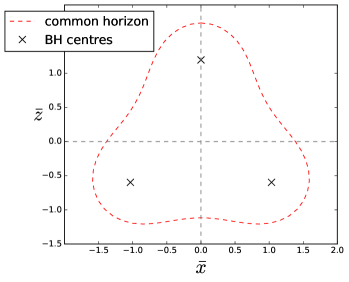
Figure 2: The apparent horizon for Brill-Lindquist equal-mass 3-blackhole spacetime at $R=1.195\approx R_{\rm crit}$. The left panel shows the cross-section (red dashed line) of the common horizon on the $\bar{x}$-$\bar{z}$ plane; the right panel is the side view of the full surface of the common horizon.

3.3 Numerical spacetimes

We prepare numerical spacetimes to further test our finder using the open source code Einstein Toolkit [27]. The simulation variables $\gamma_{ij}$ and $K_{ij}$ are post-processed to produce data on a uniform rectangular Cartesian grid before importing to our finder. In the case of dynamical binary black hole simulation where adaptive mesh refinement is turned on, we use the python package Kuibit [9] for the post-processing. We also activate the inherent apparent horizon finder in the code, AHFinderDirect [39, 40], for comparison.

3.3.1 Numerical Kerr-Schild spacetime

We first test our finder with an off-centered Kerr-Schild data. The numerical spacetime data spans the Cartesian grid space of $x,y,z\in[-2.5,2.5]$ with a grid spacing of $\Delta x=\Delta y=\Delta z=0.05$. We use a sphere of coordinate radius $1.5$ centered at the coordinate origin as the initial guess surface. We use the ILUCG matrix routines in all cases for AHFinderDirect.

Table 4: Finding the apparent horizon in numerical off-centered Kerr-Schild data with $a=0.6$ (top) and $a=0.8$ (bottom). The first column represents the resolution to describe the horizon surface. The following four columns represent the number of grid levels $n$, the relative error in the proper area $\delta A/A_{\rm Kerr}$, the number of $V$-cycle and the time (in seconds) required to locate the apparent horizon using our code. The last two columns represent the number of Newton steps and time (in seconds) required for AHFinderDirect. See text for the numerical setup of the spacetime.

• $a=0.6$	MGAHF				AHFinderDirect
  Resolution	$n$-grid	$|\delta A/A_{\rm Kerr}|$	#$V$	Time (s)	#Newton	Time (s)
  $37\times 73$  ($5\text{\,}\mathrm{\SIUnitSymbolDegree}$)	4	$2\text{\times}{10}^{-6}$	18	2.635	8	1.604
  $61\times 121$ ($3\text{\,}\mathrm{\SIUnitSymbolDegree}$)	5	$2\text{\times}{10}^{-7}$	17	6.294	8	4.180
  $91\times 181$ ($2\text{\,}\mathrm{\SIUnitSymbolDegree}$)	6	$1\text{\times}{10}^{-8}$	17	12.387	8	11.393
  $181\times 361$ ($1\text{\,}\mathrm{\SIUnitSymbolDegree}$)	7	$1\text{\times}{10}^{-8}$	18	33.802	8	88.632

• $a=0.8$	MGAHF				AHFinderDirect
  Resolution	$n$-grid	$|\delta A/A_{\rm Kerr}|$	#$V$	Time (s)	#Newton	Time (s)
  $37\times 73$  ($5\text{\,}\mathrm{\SIUnitSymbolDegree}$)	4	$2\text{\times}{10}^{-6}$	23	3.251	8	1.628
  $61\times 121$ ($3\text{\,}\mathrm{\SIUnitSymbolDegree}$)	5	$3\text{\times}{10}^{-7}$	22	7.864	8	4.170
  $91\times 181$ ($2\text{\,}\mathrm{\SIUnitSymbolDegree}$)	6	$4\text{\times}{10}^{-8}$	21	14.461	8	11.009
  $181\times 361$ ($1\text{\,}\mathrm{\SIUnitSymbolDegree}$)	7	$1\text{\times}{10}^{-7}$	21	37.178	8	87.173

We consider a black hole of unity mass and spin $a$ that is located at $(0.2,0.2,0.2)$ in Cartesian coordinates. We tabulate the results for $a=0.6$ and $a=0.8$ in Table 4. The time to locate the solution surface mainly depends on two factors—the overall convergence of the algorithm and the computational cost within each iteration. The convergence order of the algorithm is important in the sense that as many as 30 interpolations for the geometric variables are required at every grid point at each (outer) iteration. Since we adopt a pure multigrid algorithm, which has a slower convergence than the quadratic convergence in Newton’s method, one can see that our finder needs more iterations (number of $V$-cycles) for convergence, so more time is spent on the interpolation routines when compared to AHFinderDirect. Notice that the number of iterations is insensitive to the resolution used for fixed $a$. Had we used the pointwise Gauss-Seidel relaxation as the smoothing operator, the number of iterations would grow linearly with the number of grid points, and the speed of the code would become very slow due to the large amount of interpolations required.

At high resolutions, however, we find that our finder generally locates the apparent horizon faster than AHFinderDirect. This is somewhat expected because, at a rough estimation, the operation cost of performing the matrix LU decomposition of the Jacobian equation in AHFinderDirect is $\mathcal{O}(N^{3})$ but that of one multigrid cycle is $\mathcal{O}(N)$, where $N$ is the total number of grid points used to describe the horizon surface and $N{=}$$N_{\theta}\times N_{\phi}$ in our case. The total search time is a competition between the two factors mentioned above. The computational cost of each iteration becomes more important with increasing resolutions. Although the overall convergence rate of our multigrid algorithm is not as fast as Newton’s method, there is a critical resolution at which our multigrid algorithm starts to work faster. In particular, our finder can be more than two times faster when the angular separation between two neighboring grids is about $1\text{\,}\mathrm{\SIUnitSymbolDegree}$ as shown in Table 4. We have performed the same test for additional values of the spin parameter $a$ at $1\text{\,}\mathrm{\SIUnitSymbolDegree}$ resolution, and the runtimes are plotted in Figure 3. Although the runtime of our finder grows with $a$, it takes lesser time to converge in all cases. Recall that the performance of our finder has extra dependence on the convergence parameter $\eta$. At the extreme case of $a=0.99$, the optimal value of $\eta$ shifts to around 1.45, and the runtime is reduced by half comparing to the case $\eta=0.8$.

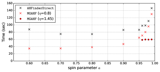
Figure 3: Comparison between our finder and AHFinderDirect on the runtime to locate the apparent horizon in numerical off-centered Kerr-Schild data with different values of spin parameter $a$. A spherical surface of radius 1.6 centered at the coordinate origin is used as the initial guess. The angular resolution for the runs is $1\text{\,}\mathrm{\SIUnitSymbolDegree}$. The rightmost 4 sets of data points correspond to $a=0.96,0.97,0.98,0.99$.

We further test on the case where the spin parameter is $a=0.99$, but with the black hole relocated to $(0.2,0.2,0)$. The initial guesses are spherical surfaces centered at the coordinate origin as before, with radius $r_{0}$ ranging from 1.5 to 1.6 with increments of 0.01. We found that AHFinderDirect is more volatile to the initial guess surface, and is able to find the apparent horizon only at $r_{0}=1.54,1.57,1.58$ and $1.6$ (it fails to converge otherwise). On the other hand, our finder is able to find the correct solution for all these cases.

3.3.2 Dynamical binary black hole spacetime

We simulate the merger of an unequal-mass black hole binary using Einstein Toolkit [27]. The initial mass ratio of the two non-spinning black holes is set to be $q\simeq 0.7$. We use standard evolution schemes and gauge conditions, with multiple layers of mesh refinements to perform the simulation. The finest grids of grid spacing $\Delta x=\Delta y=\Delta z=0.03125$ cover the two black holes at all times. We export the numerical data to an uniform grid of the finest grid spacing by Kuibit [9] to search for the horizons using our finder. For the two individual horizons, the local coordinate origin is chosen by the position of singularity provided by the PunctureTracker thorn in the simulation code, while that of the common apparent horizon is simply set to be the origin of the simulation grid.

Table 5: Comparison between our finder and AHFinderDirect on the proper areas of the individual horizons and the common apparent horizon found in merging binary black hole spacetime. The relative difference is reported in the last column.

• 	MGAHF	AHFinderDirect	$|\delta A/A|$
  Horizon of $m_{1}$	19.0239	19.0097	$7\text{\times}{10}^{-4}$
  Horizon of $m_{2}$	9.4808	9.4671	$1\text{\times}{10}^{-3}$
  Common apparent horizon	39.8666	39.8691	$6\text{\times}{10}^{-5}$

Figure 4: The common apparent horizon and the individual horizons found by our finder in a dynamical spacetime of merging unequal-mass black hole binary at a time when the common apparent horizon first appears.

We report the results of horizon finding at the simulation time when the common apparent horizon first appears in Table 5 and the corresponding snapshot of the three horizon surfaces in Figure 4. The horizon surfaces are modeled by $5\text{\,}\mathrm{\SIUnitSymbolDegree}$ angular resolution ($N_{\theta}{\times}N_{\phi}=37{\times}73$). In Figure 4, the common apparent horizon is represented by the purple surface, inside of which are the two individual horizons represented by the green and blue surfaces. In terms of the proper areas, our finder agrees with the default AHFinderDirect in the simulation code to within $0.2\%$. The difference is the biggest for the horizon of the smaller black hole, as the spherical grids become overly stacked at that radius.

4 Conclusions

We have presented a new apparent horizon searching algorithm using a multigrid method in this work. We have evaluated the performance of our finder on analytic spacetimes, including the Brill-Lindquist data with two or three black holes. We have recovered the results of the critical parameter for a common apparent horizon to appear in these spacetimes. We have also tested our finder on numerical spacetimes, namely the off-centered Kerr-Schild data and the inspiraling binary black hole spacetime. We have demonstrated that, in terms of speed, the multigrid searching algorithm begins to outperform the currently fastest algorithm (Thornburg’s AHFinderDirect [39, 40]) at high resolutions. We have also shown that our finder is capable of capturing the first appearance of the common apparent horizon in merging black hole binary simulation.

From a numerical perspective of viewing our finder as a general multigrid solver for Poisson equations in spherical coordinates, there are some notable aspects. We have verified that the line relaxation scheme is preferable (in terms of convergence) to a pointwise relaxation scheme, even when dealing with a solution-dependent nonlinear source term. We have derived the (semi-)compact 4th order finite difference scheme for solving the spherical Poisson equation. The derivation follows a similar procedure used for Cartesian grids (see [19] and references therein). Our study demonstrates the applicability of this scheme in reducing the complexity of a line relaxation technique on spherical coordinates, from a penta-diagonal matrix inversion to a more efficient tri-diagonal matrix inversion. We believe the formula derived should be directly applicable to other 2-dimensional Poisson equations on the sphere.

We make some final remarks on how our multigrid algorithm can be further improved. First, the segment relaxation scheme (See Section 2.3) could be used to improve the convergence. We only use $\phi$-line relaxation as the smoother in our multigrid solver, but the line relaxation direction is preferred to be aligned with the anisotropy direction in the differential operator as it could give better convergence [5]. Second, using a variant multigrid algorithm might also improve the convergence. We solve the non-linear apparent horizon equation by turning it into a linear elliptic equation with a non-linear source term. In this way, the nonlinearity of the principle equation is avoided. However, by not addressing it directly, the rate of convergence could be compromised. The common multigrid methods to tackle nonlinearity directly are the full approximation scheme [10] or Newton-multigrid [12] algorithm. We have not adopted these methods in the current work since they in principle bring up technical implementation issues in the case of the apparent horizon equation. Exploring these alternative multigrid schemes could be one future investigation direction for increasing the efficiency of our multigrid code.

Data availability statement

No new data were created or analyzed in this study.

ORCID iDs

Hon-Ka Hui  https://orcid.org/0000-0002-2815-527X
Lap-Ming Lin  https://orcid.org/0000-0002-4638-5044

References

Appendix A Fully-compact 4th-order finite difference scheme for spherical Poisson equations

Suppose we solve a general Poisson equation in spherical coordinates,

$$\left(\frac{\partial^{2}}{\partial\theta^{2}}+\cot\theta\frac{\partial}{\partial\theta}+\frac{1}{\sin^{2}\theta}\frac{\partial^{2}}{\partial\phi^{2}}\right)u(\theta,\phi)=f(\theta,\phi),$$ (33)

on a spherical grid of grid size $h=\Delta\theta$ and $k=\Delta\phi$. Using a 2nd-order finite difference approximation, the first two terms on the left side are

$$\frac{\partial^{2}u}{\partial\theta^{2}}+\cot\theta\frac{\partial u}{\partial\theta}=\left(\frac{\partial^{2}u}{\partial\theta^{2}}+\cot\theta\frac{\partial u}{\partial\theta}\right)_{\rm FD2}-\frac{h^{2}}{12}\left(\frac{\partial^{4}u}{\partial\theta^{4}}+2\cot\theta\frac{\partial^{3}u}{\partial\theta^{3}}\right)+\mathcal{O}(h^{4}).$$ (34)

We then seek an expression to replace the third and fourth order derivatives in the second parenthesis. Differentiating (33) w.r.t $\theta$ gives

$$\frac{\partial^{3}u}{\partial\theta^{3}}+\cot\theta\frac{\partial^{2}u}{\partial\theta^{2}}-\frac{1}{\sin^{2}\theta}\frac{\partial u}{\partial\theta}-\frac{2\cos\theta}{\sin^{3}\theta}\frac{\partial^{2}u}{\partial\phi^{2}}+\frac{1}{\sin^{2}\theta}\frac{\partial^{3}u}{\partial\theta\partial\phi^{2}}=\frac{\partial f}{\partial\theta}.$$ (35)

The second derivative reads

$$\frac{\partial^{4}u}{\partial\theta^{4}}+\cot\theta\frac{\partial^{3}u}{\partial\theta^{3}}-\frac{2}{\sin^{2}\theta}\frac{\partial^{2}u}{\partial\theta^{2}}+\frac{2\cos\theta}{\sin^{3}\theta}\frac{\partial u}{\partial\theta}+\frac{6-4\sin^{2}\theta}{\sin^{4}\theta}\frac{\partial^{2}u}{\partial\phi^{2}}$$

$$-\frac{2\cos\theta}{\sin^{3}\theta}\frac{\partial^{3}u}{\partial\theta\partial\phi^{2}}-\frac{2\cos\theta}{\sin^{3}\theta}\frac{\partial^{3}u}{\partial\theta\partial\phi^{2}}+\frac{1}{\sin^{2}\theta}\frac{\partial^{4}u}{\partial\theta^{2}\partial\phi^{2}}=\frac{\partial^{2}f}{\partial\theta^{2}}.$$ (36)

Combining the last two equations, we have

$$\frac{\partial^{4}u}{\partial\theta^{4}}+2\cot\theta\frac{\partial^{3}u}{\partial\theta^{3}}={} \left(\cot\theta\frac{\partial f}{\partial\theta}+\frac{\partial^{2}f}{\partial\theta^{2}}\right)+\left(1+\frac{1}{\sin^{2}\theta}\right)\frac{\partial^{2}u}{\partial\theta^{2}}-\frac{\cos\theta}{\sin^{3}\theta}\frac{\partial u}{\partial\theta}$$ (37)

$$+\frac{2\sin^{2}\theta-4}{\sin^{4}\theta}\frac{\partial^{2}u}{\partial\phi^{2}}+\frac{3\cos\theta}{\sin^{3}\theta}\frac{\partial^{3}u}{\partial\theta\partial\phi^{2}}-\frac{1}{\sin^{2}\theta}\frac{\partial^{4}u}{\partial\theta^{2}\partial\phi^{2}}.$$

The right hand side of this equation can be evaluated by 2nd order finite difference approximation and be substituted back to (34) while the overall error is maintained at $\mathcal{O}(h^{4})$. We can then combine the result with (24) to obtain the fully-compact 4th order finite difference approximation for the spherical Poisson equation (33). The explicit expression is

$$\left(\frac{\partial^{2}u}{\partial\theta^{2}}+\cot\theta\frac{\partial u}{\partial\theta}\right)_{\rm FD2}+\left(\frac{1}{\sin^{2}\theta}\frac{\partial^{2}u}{\partial\phi^{2}}\right)_{\rm FD2}-\frac{k^{2}}{12}\left[\frac{\partial^{2}f}{\partial\phi^{2}}-\frac{\partial^{4}u}{\partial\theta^{2}\partial\phi^{2}}-\cot\theta\frac{\partial^{3}u}{\partial\theta\partial\phi^{2}}\right]_{\rm FD2}$$

$$-\frac{h^{2}}{12}\Bigg{[}\cot\theta\frac{\partial f}{\partial\theta}+\frac{\partial^{2}f}{\partial\theta^{2}}+\left(1+\frac{1}{\sin^{2}\theta}\right)\frac{\partial^{2}u}{\partial\theta^{2}}-\frac{\cos\theta}{\sin^{3}\theta}\frac{\partial u}{\partial\theta}+\frac{2\sin^{2}\theta-4}{\sin^{4}\theta}\frac{\partial^{2}u}{\partial\phi^{2}}$$

$$+\frac{3\cos\theta}{\sin^{3}\theta}\frac{\partial^{3}u}{\partial\theta\partial\phi^{2}}-\frac{1}{\sin^{2}\theta}\frac{\partial^{4}u}{\partial\theta^{2}\partial\phi^{2}}\Bigg{]}_{\rm FD2}+\mathcal{O}(h^{4},h^{2}k^{2},k^{4})\quad=f.$$ (38)

References

- [1] Alcubierre M, Brügmann B, Diener P, Koppitz M, Pollney D, Seidel E and Takahashi R 2003 Phys. Rev. D 67(8) 084023
- [2] Ashtekar A and Krishnan B 2003 Phys. Rev. D 68(10) 104030
- [3] Ashtekar A and Krishnan B 2004 Living Reviews in Relativity 7 1–91
- [4] Baiotti L and Rezzolla L 2006 Phys. Rev. Lett. 97(14) 141101
- [5] Barros S R 1991 Journal of Computational Physics 92 313–348
- [6] Baruch G, Fibich G and Tsynkov S 2009 Journal of Computational Physics 228 3789–3815
- [7] Baumgarte T W, Cook G B, Scheel M A, Shapiro S L and Teukolsky S A 1998 Phys. Rev. D 57(12) 7299–7311
- [8] Baumgarte T W and Shapiro S L 2010 Numerical Relativity: Solving Einstein’s Equations on the Computer (Cambridge University Press)
- [9] Bozzola G 2021 The Journal of Open Source Software 6 3099
- [10] Brandt A 1977 Mathematics of computation 31 333–390
- [11] Brandt S and Brügmann B 1997 Phys. Rev. Lett. 78(19) 3606–3609
- [12] Briggs W L, Henson V E and McCormick S F 2000 A multigrid tutorial (SIAM)
- [13] Brill D R and Lindquist R W 1963 Phys. Rev. 131(1) 471–476
- [14] Britt S, Tsynkov S and Turkel E 2010 Journal of Scientific Computing 45 26–47
- [15] Cheong P C K, Lin L M and Li T G F 2020 Classical and Quantum Gravity 37 145015
- [16] Choptuik M and Unruh W G 1986 General relativity and gravitation 18 813–843
- [17] Collatz L 1960 The numerical treatment of differential equations (Springer Berlin, Heidelberg)
- [18] Cook G B, Choptuik M W, Dubal M R, Klasky S, Matzner R A and Oliveira S R 1993 Phys. Rev. D 47(4) 1471–1490
- [19] Deriaz E 2020 BIT Numerical Mathematics 60 199–233
- [20] East W E, Ramazanoğlu F M and Pretorius F 2012 Phys. Rev. D 86(10) 104053
- [21] Evans C, Ferguson D, Khamesra B, Laguna P and Shoemaker D 2020 Classical and Quantum Gravity 37 15LT02
- [22] Ge Y 2010 Journal of Computational Physics 229 6381–6391
- [23] Hackbusch W 1985 Multi-Grid Methods and Applications Springer Series in Computational Mathematics, 4 (Springer Berlin, Heidelberg)
- [24] Hawking S W and Ellis G F R 1973 The Large Scale Structure of Space-Time Cambridge Monographs on Mathematical Physics (Cambridge University Press)
- [25] Lai M C and Tseng J M 2007 Journal of Computational and Applied Mathematics 201 175–181
- [26] Lin L M and Novak J 2007 Classical and Quantum Gravity 24 2665
- [27] Löffler F, Faber J, Bentivegna E, Bode T, Diener P, Haas R, Hinder I, Mundim B C, Ott C D, Schnetter E, Allen G, Campanelli M and Laguna P 2012 Classical and Quantum Gravity 29 115001
- [28] Misner C W, Thorne K S and Wheeler J A 1973 Gravitation (Macmillan)
- [29] Moldenhauer N, Markakis C M, Johnson-McDaniel N K, Tichy W and Brügmann B 2014 Phys. Rev. D 90(8) 084043
- [30] Penrose R 1965 Phys. Rev. Lett. 14(3) 57–59
- [31] Pook-Kolb D, Birnholtz O, Krishnan B and Schnetter E 2019 Phys. Rev. D 99(6) 064005
- [32] Pook-Kolb D, Hennigar R A and Booth I 2021 Phys. Rev. Lett. 127(18) 181101
- [33] Prasad V, Gupta A, Bose S, Krishnan B and Schnetter E 2020 Phys. Rev. Lett. 125(12) 121101
- [34] Press W H, Teukolsky S A, Vetterling W T and Flannery B P 2007 Numerical recipes 3rd edition: The art of scientific computing (Cambridge university press)
- [35] Schnetter E 2003 Classical and Quantum Gravity 20 4719
- [36] Schnetter E, Krishnan B and Beyer F 2006 Phys. Rev. D 74(2) 024028
- [37] Shibata M 1997 Phys. Rev. D 55(4) 2002–2013
- [38] Sykes B, Mueller B, Cordero-Carrión I, Cerdá-Durán P and Novak J 2023 Phys. Rev. D 107(10) 103010
- [39] Thornburg J 1996 Phys. Rev. D 54(8) 4899–4918
- [40] Thornburg J 2003 Classical and Quantum Gravity 21 743
- [41] Thornburg J 2007 Living Reviews in Relativity 10 1–68
- [42] Trottenberg U, Oosterlee C W and Schuller A 2000 Multigrid (Elsevier)
- [43] Wesseling P 1992 An introduction to multigrid methods (Wiley)
- [44] Zhang J 2002 Journal of Computational Physics 179 170–179