∎
22email: susanna.parenti@ias.u-psud.fr 33institutetext: I. Chifu 44institutetext: Institute for Astrophysics, University of Göttingen, Friedrich-Hund-Platz 1, 37077 Göttingen, Germany,
Max-Planck-Institut für Sonnensystemforschung, Justus-von-Liebig-Weg 3 37077 Göttingen, Germany 55institutetext: G. Del Zanna 66institutetext: DAMTP, Centre for Mathematical Sciences, University of Cambridge, Wilberforce Road, Cambridge CB3 0WA UK 77institutetext: Justin Edmondson 88institutetext: Department of Climate and Space Sciences and Engineering, University of Michigan, Ann Arbor, MI 48109, USA 99institutetext: Alessandra Giunta 1010institutetext: RAL Space, UKRI STFC Rutherford Appleton Laboratory, Harwell, Didcot, OX11 0QX, United Kingdom 1111institutetext: Viggo H. Hansteen 1212institutetext: Institute of Theoretical Astrophysics, University of Oslo, P.O. Box 1029 Blindern, 0315 Oslo, Norway 1313institutetext: Aleida Higginson 1414institutetext: Department of Climate and Space Sciences and Engineering, University of Michigan, Ann Arbor, MI 48109, USA 1515institutetext: J. M. Laming 1616institutetext: Space Science Division, Code 7684, Naval Research Laboratory, Washington, DC 20375, USA 1717institutetext: S. T. Lepri 1818institutetext: Department of Climate and Space Sciences and Engineering, University of Michigan, Ann Arbor, MI 48109, USA 1919institutetext: B. J. Lynch 2020institutetext: Space Sciences Laboratory, University of California–Berkeley, Berkeley, CA 94720, USA 2121institutetext: Y. J. Rivera 2222institutetext: Center for Astrophysics, Harvard University, 60 Garden Street, Cambridge, MA 02138, USA 2323institutetext: R. von Steiger 2424institutetext: International Space Science Institute, Hallerstrasse 6, 3012 Bern, Switzerland
Physikalisches Institut, University of Bern, Sidlerstrasse 5, 3012 Bern, Switzerland 2525institutetext: T. Wiegelmann 2626institutetext: Max-Planck-Institut für Sonnensystemforschung, Justus-von-Liebig-Weg 3, 37077 Göttingen, Germany 2727institutetext: Robert F. Wimmer-Schweingruber 2828institutetext: Institute of Experimental and Applied Physics, University of Kiel, Leibnizstrasse 11, D-24118 Kiel, Germany 2929institutetext: Natalia Zambrana Prado 3030institutetext: Institut d’Astrophysique Spatiale, CNRS-Université Paris-Saclay, 91405 Orsay, France 3131institutetext: Gabriel Pelouze 3232institutetext: Centre for mathematical Plasma Astrophysics, Department of Mathematics, KU Leuven, Celestijnenlaan 200B bus 2400, 3001 Leuven, Belgium
Linking the Sun to the Heliosphere Using Composition Data and Modelling
Abstract
Our understanding of the formation and evolution of the corona and the heliosphere is linked to our capability of properly interpret the data from remote sensing and in–situ observations. In this respect, being able to correctly connect in–situ observations with their source regions on the Sun is the key for solving this problem. In this work we aim at testing a diagnostics method for this connectivity.
This paper makes use of a coronal jet observed on 2010 August 2nd in active region 11092 as a test for our connectivity method. This combines solar EUV and in–situ data together with magnetic field extrapolation, large scale MHD modeling and FIP (First Ionization Potential) bias modeling to provide a global picture from the source region of the jet to its possible signatures at 1AU.
Our data analysis reveals the presence of outflow areas near the jet which are within open magnetic flux regions and which present FIP bias consistent with the FIP model results. In our picture, one of these open areas is the candidate jet source. Using a back-mapping technique we identified the arrival time of this solar plasma at the ACE spacecraft. The in–situ data show signatures of changes in the plasma and magnetic field parameters, with FIP bias consistent with the possible passage of the jet material.
Our results highlight the importance of remote sensing and in–situ coordinated observations as a key to solve the connectivity problem. We discuss our results in view of the recent Solar Orbiter launch which is currently providing such unique data.
Keywords:
Active region Solar wind Connectivity Diagnostics Modelling UV emission in–situ data1 Introduction
It is well acknowledged that the interplanetary medium is filled by the spatial expansion of the solar magnetic field embedded to a continuous flow of particles, the solar wind; these are the main ingredients of the heliosphere.
The first indirect evidence of the presence of the solar wind dates back to the beginning of the twentieth century, while the first in-situ wind and magnetic field measures are from the early 1960 (see for instance Hundhausen (1972) for an historical review). Since then, enormous progress has been made, both for the spatial and temporal monitoring of the heliosphere and the theoretical explanation of its origin and evolution (see for instance Hansteen and Velli, 2012; Abbo et al., 2016). For instance, the initial prediction for the solar wind (Parker, 1958) envisaged a wind driven by thermal forces originating in a MHD wave heated corona. The modern view is more that the MHD waves couple to the nascent solar wind directly to cause its acceleration. The role of interchange reconnection also appears to be a good candidate for releasing plasma into open regions to feed the solar wind (see for instance Abbo et al. (2016)).
The solar wind is comprised of two basic regimes (e.g. McComas et al., 2003). The fast wind, with typical speed km s-1 is relatively steady, exhibits Alfvénic turbulence, is established to originate in coronal holes, and corresponds the closest to Parker’s original idea (e.g. Ko et al., 2018). The slow wind km s-1 is much more variable, exhibits periods of Alfvénic and non-Alfvénic turbulence (e.g. Ko et al., 2018), has composition similar to coronal loops (e.g. Heber et al., 2021), and has less certain solar origins. Prior observations suggest that solar wind ions are heated in open magnetic field by microscopic (kinetic) wave-particle processes, as the plasma becomes collisionless. SOHO/UVCS (Solar and Heliosheric Observatory, Ultraviolet Coronagraph Spectrometer) showed pronounced kinetic anisotropies (with ) for O5+ and Mg9+ in polar coronal holes (Kohl et al., 1997, 1998, 2006; Cranmer et al., 1999, 2008) and streamers above 1.9 R⊙ (Frazin et al., 1999). Interchange reconnection may also play a role in supplying material into the slow solar wind, as well, with material previously trapped on coronal loops (Fisk and Schwadron, 2001; Edmondson et al., 2010).
The global properties of the heliosphere are quite well understood, however there are several not well understood aspects of the smaller scales. One example is the identification at the Sun of the small scale wind source regions. To fully understand the structure and dynamics of the heliosphere requires modelling and simulation capabilities to create an evolving 3D environment validated by continuous, widely distributed observations. Ground and space based data sets are critical to constraining our understanding of the spatial and temporal conditions in this 3D environment. Both in–situ and remote sensing observations provide critical vantage points to view structures and phenomena on the Sun, in the corona, as well as observe their propagation through the heliosphere. Due to the limited number of satellite and ground based observations, incomplete spatial mapping from the Sun out into the heliosphere requires new methods for connecting observations (see for instance Stansby et al., 2020; de Pablos et al., 2021). Connecting measurements from the Sun into the heliosphere is a major challenge in solar physics and heliophysics, not only in that different quantities are observed with different sensors, at different time cadences, but also the connections between these measurements often do not have a well defined or unique solution (see for instance Poletto et al., 1996). In order to connect structures at the Sun with those observed in–situ, one must ensure that the same magnetic structure is sampled by both methods. Spatial (due to the deformation of the magnetic field as it expands in the heliosphere) and the temporal changes (due to the delay between the moment of surface escape and the in–situ spacecraft crossing) of such magnetic structures have to be taken into account. Several methods can be used to back map in–situ measurements (see for instance Neugebauer et al., 1998) and their comparison made in Peleikis et al. (2017) or Kruse et al. (2021), but each have their limitations. An example of this kind of effort was made during the periodic quadrature between the SOHO satellite (Domingo et al., 1995) and the Ulysses mission (Wenzel et al., 1992). In this period it was possible to derive the plasma parameters from the Sun, to the corona (e.g. density, temperature, composition, outflows) up to several solar radii, and try to link them to the same parameters measured in–situ (e.g. Suess and Poletto, 2001; Parenti et al., 2003; Bemporad et al., 2003).
One of the most promising methods for back-mapping heliospheric structures to their solar counterparts involves observing the compositional properties including the ionization states of heavy ions as well as their elemental abundances, sorted by a property called the First Ionization Potential (FIP) bias. While kinetic properties of the solar wind are affected by propagation effects such as cooling, the heavy ion properties are determined in the low corona and do not evolve as the solar wind transits through the heliosphere. The FIP bias describes the variation of the fractionation of the chemical composition of heavy elements which occurs between the photosphere and regions further out in the corona (e.g. Sheeley, 1995; Feldman, 1992). In particular, elements with FIP lower than about 10 eV (e.g. Mg, Si, Fe) are observed to be enhanced compared to those with higher FIP (e.g. O, Ne, Ar), with respect to their photospheric values. This bias has different amplitudes depending on the plasma/magnetic structure observed. It was first detected in the solar wind, with an amplitude of on average 2–3 for slow wind, and around 1–1.5 for the fast wind and has served as a key discriminator between these two types of wind (e.g. Geiss et al., 1995; von Steiger et al., 2000; Zurbuchen et al., 2012).
Variations of the FIP bias were also inferred in different parts of the Sun and in the corona (Raymond et al., 1997; Parenti et al., 2000, 2019), showing temperature dependence (e.g. Del Zanna, 2019). In active regions (ARs), which are considered one of the candidate locations for the nascent slow wind and which are the subject of our work, the FIP bias is quite variable and both coronal (FIP bias 2) or photospheric composition can be found (see for instance the review in Del Zanna and Mason, 2018). This variation also includes the increase of FIP bias with the ARs lifetime (e.g. Ko et al., 2016; Harra et al., 2021) and/or with the emergence of new flux (e.g. Baker et al., 2018). The range of variability in the corona can be higher than that observed in the wind, because at 1 AU the wind may include a mixture of different solar wind structures. It has to be noticed that the various methodologies used to derive the bias may affect the results, which may contribute to the origin of the inferred variability of the FIP effect (see for instance the discussion in Del Zanna et al., 2015).
In addition to the FIP bias, in–situ heavy ion charge state measurements can also be used as a tool to investigate coronal heating processes that accelerate the steady-state slow and fast solar wind (e.g. Hundhausen et al., 1968; Owocki et al., 1983; Bürgi and Geiss, 1986; Ko et al., 1997; von Steiger et al., 1997; Wimmer-Schweingruber et al., 1997, 1999; von Steiger et al., 2000; Zurbuchen et al., 2002; Laming and Lepri, 2007; von Steiger and Zurbuchen, 2011; Landi et al., 2012; Zurbuchen et al., 2012; Lepri et al., 2013; Zhao et al., 2017a, b). The same techniques have been implemented in transients to investigate and place constraints on the thermal history of plasma as it accelerates through the corona (e.g. Gruesbeck et al., 2011; Rivera et al., 2019b, a). The heavy ion charge states in the solar wind can reflect the plasma properties of the inner corona where the solar wind originates. As the solar wind is accelerated, the electron number density rapidly decreases with distance from the Sun, while the electron temperature increases and reaches a maximum value before decreasing again (Kohl et al., 2006; Laming, 2004a). The ionization and recombination rates for a given pair of charge states of an element are proportional to the electron density and also depend on electron temperature (or kinetic energy), so they also rapidly decrease with increasing height in the corona. As the plasma parcel accelerates through the corona it will reach a critical height where the electron density is so low that the time scale to modify the charge states exceeds the expansion time scale and the ionization state of an element remains unaltered (Owocki et al., 1983) as the solar wind continues to propagate through the corona (Landi et al., 2012). This process is called the “freeze-in” process. Beyond the freeze-in point, located at depending on which ion pair is considered (Laming, 2004a; Laming and Lepri, 2007), the charge state distributions of heavy ions (e.g. C, N, O, Si, Mg, Fe) thus maintain a record of the thermal properties of the plasma in the inner corona and carry with them this information as the solar wind propagates throughout the heliosphere.
The ESA-NASA Solar Orbiter mission (launched in February 2020, Müller et al., 2020) has been designed to strongly contribute to solve the connectivity problem between remote and in–situ measurements below 1 AU. The mission profile is designed to reduced the gap between in–situ and remote sensing measurements, by approaching to the Sun up to a distance of about 0.3 AU, while additionally providing periods of near-corotation. Some of the on board remote sensing instruments, the Spectral Imaging of the Coronal Environment (SPICE, Spice Consortium et al. (2020)), the Extreme Ultraviolet Imager (EUI, Rochus et al. (2020)), the Polarimetric and Helioseismic Imager (PHI, Solanki et al. (2020)) and the Spectrometer Telescope for Imaging X-rays (STIX, Krucker et al. (2020)) will observe the source regions at the Sun that will ultimately be sampled a few days later by the on board in–situ instruments. The spacecraft will locally sample the solar wind which has just been accelerated (Owen et al., 2020), and observe the heliospheric structures formed in the corona. Close to the Sun, the plasma and magnetic field properties have only been partially modified by propagation effects and interactions with nearby heliospheric structures, thus reducing the uncertainties in connecting these structures back to their sources. The payload instruments are designed to provide a wide complement of measurements to solve this connectivity problem below 1 AU. The Solar Orbiter activity comes to complement the existing measurements at 1 AU, which are needed for the solar connectivity at this distance, as the dominant physical processes may not be the same. We need to sample the environment over different physical conditions to test our heliospheric models in order to advance in our knowledge of the whole Sun-heliospheric system. Furthermore, the opportunity to have available measurements at different solar distance should be accompanied by the evolution and optimization of the diagnostics for multi-instrument observations.
This paper presents an initial attempt to utilize both remote sensing and in–situ measurements at 1 AU, along with a full complement of modelling techniques, to illustrate the methods required to solve the connectivity problem that will also be addressed by Solar Orbiter at the beginning of 2022, when the nominal mission phase will start. To this purpose we present a test case using coronal jet data to provide information on a coronal structure to connect out into the heliosphere.
AR jets are impulsive and collimated eruptions which are seen statistically observed to emerge primarily from the western periphery of the leading sunspot in a sunspot pair (Shimojo et al., 1996). Magnetic reconnection following magnetic field emergence or cancellation appears to be one of the main drivers of these plasma eruptions (Mulay et al., 2016, and references therein). A few studies have analyzed the possible correlation between AR jets and interplanetary radio III bursts observed co-temporally with these events. The conclusion is that indeed, accelerated electron beams escape the jet region (e.g. Innes et al., 2011; Mulay et al., 2016; Paraschiv and Donea, 2019), as well as impulsive solar energetic particles (see for instance Lin, 1970; Reames et al., 1985; Bučík, 2020).
UV AR jets are seen to extend into the corona up to about 2 R⊙ and magnetic field extrapolations suggest they are ejected in open field regions within the AR (Innes et al., 2011; Mulay et al., 2016). The detection of in–situ signatures of an AR jet has been attempted in the past, but with no clear results (see for instance Corti et al., 2007; Raouafi et al., 2016).
Based on our present knowledge of coronal jets and their expected signatures in the interplanetary region, we consider them as good candidates for testing connectivity diagnostics. In this paper we propose a methodology that will utilize FIP bias to connect the solar structure with the heliospheric counterpart, based on both data and modelling, and which may have a direct application for the Solar Orbiter Mission.
The paper is organized as follows: after a general introduction to the jet event in Section 2, we describe all the building blocks for the connectivity in Sect. 3. These include the use and comparison of different models for the reconstruction the coronal magnetic field, as well as the comparison of different FIP bias estimation methods. Section 4 presents the results from the modeling and data analysis while we draw our conclusions in Sect. 5.
2 The 2nd of August 2010 Solar Jet
The jet we select for our connectivity study was chosen because it had one of the most complete data coverage in time (three days around the jet) and space for the EUV observations, as well as the interplanetary signature as radio type-III burst and in–situ.
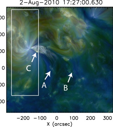
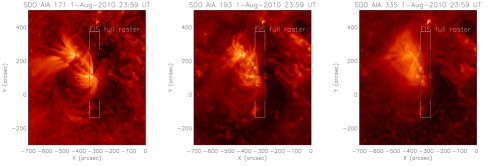
To better understand the evolution of the AR environment before, during and after the eruption, we show some context images in Figures 1 and 2. The jet occurred on August 2, 2010 in the AR 11092 between 17:10 and 17:35 UT, as seen in the AIA 171 channel and STEREO (Solar TErrestrial RElations Observatory) EUVI (Extreme UltraViolet Imager) (Figure 1).
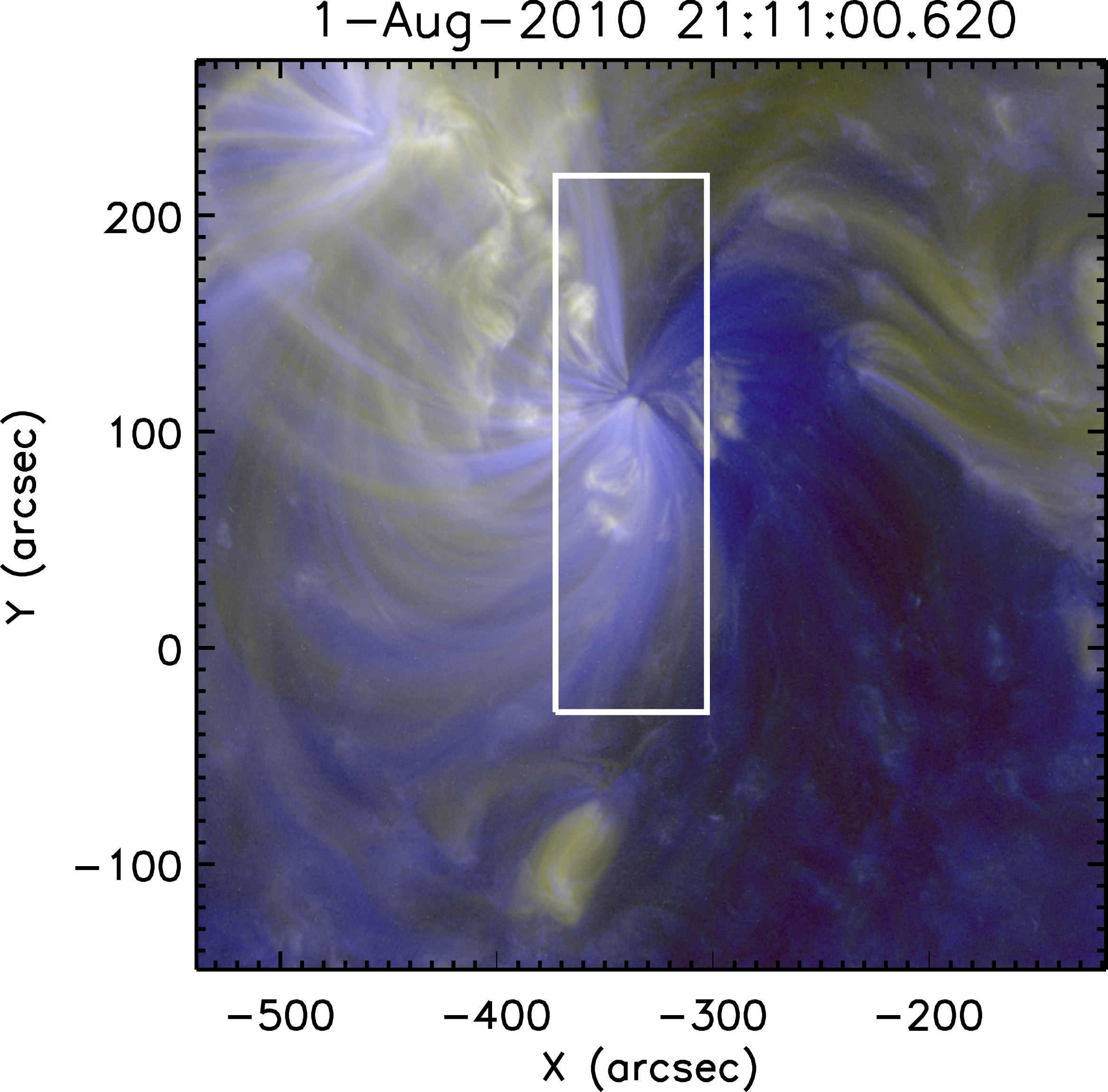
The pre–erupting corona is instead shown in the left panel of Figure 2. Here we superposed three images from AIA, representing roughly the corona at 0.9 MK (green, 171 channel), 1.5 MK (blue, 193 channel) and 2 MK (red, 211 channel). The image shows the AR the day before the eruption at close time when two of the EIS rasters used for our analysis were taken (’A’ and ’B’, see Table 1). The multi color image reflects the multi-temperature property of the AR. The half left side of the AR is made of low lying ’hot’ () loops and ’warm’ () loops arcade above them. The north west side is made of mostly hot loops while the mid-south part contains low, large scale warm loops. This latter is probably a low density and low temperature area with a magnetic structure which opened up during the jet. This is the escaping channel of the jet.
This jet was analysed in detail by Mulay et al. (2016) who studied its possible relation with the observed interplanetary radio type-III burst using WIND data. The authors identified the footpoints of the jet in the spot and in one of the small loops just at the west side of it (labeled ’C’ in Figure 2). Among the observed signatures of the dynamics in this area, they noticed flux emergence and cancellation prior to the eruption, cool H material ejected at the same time of the coronal material, and hard HXR emission from RHESSI (Reuven Ramaty High Energy Solar Spectroscopic Imager, see their Figure 5). These are clear signatures of ongoing magnetic reconnection and plasma ejection.
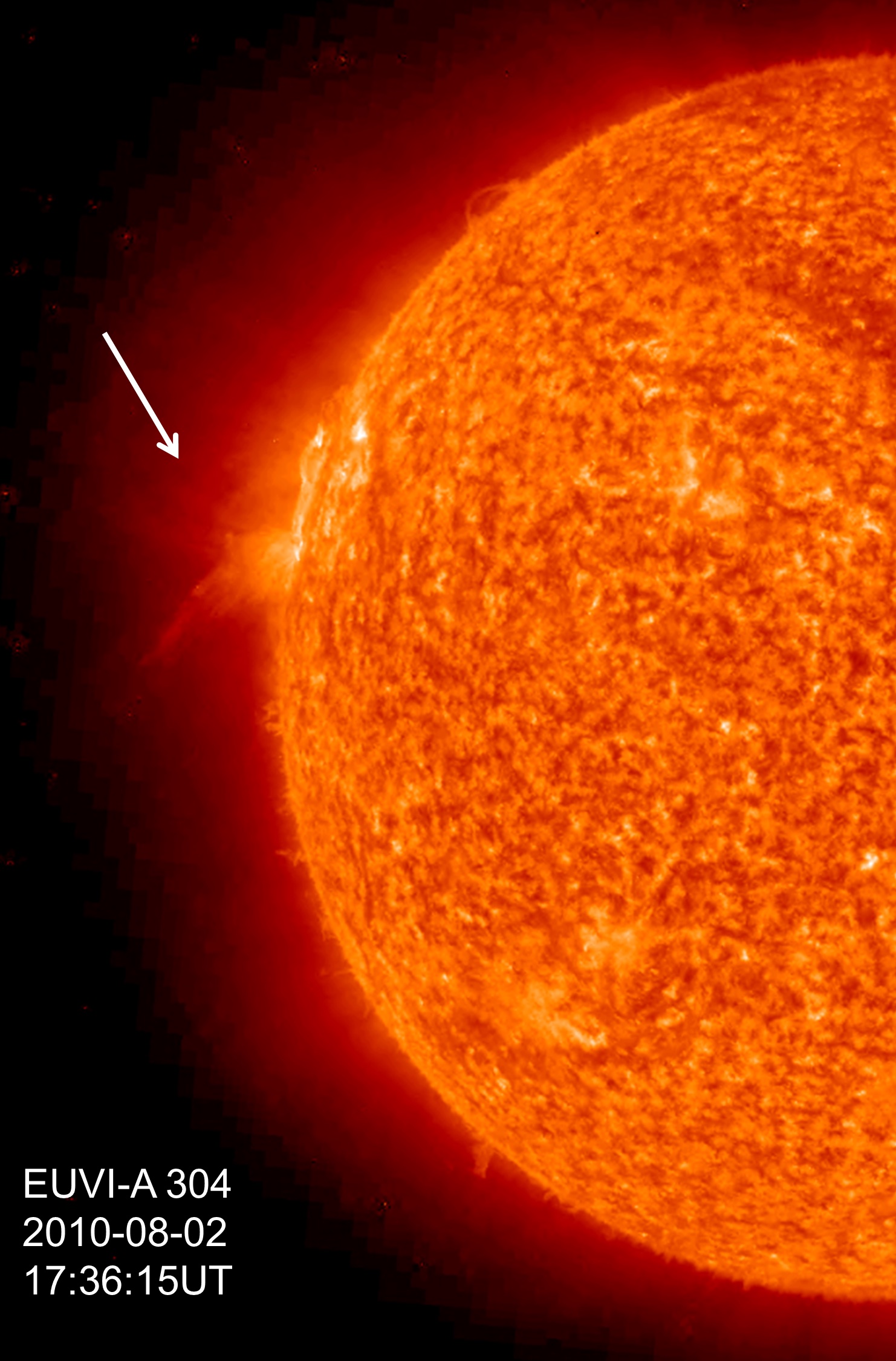
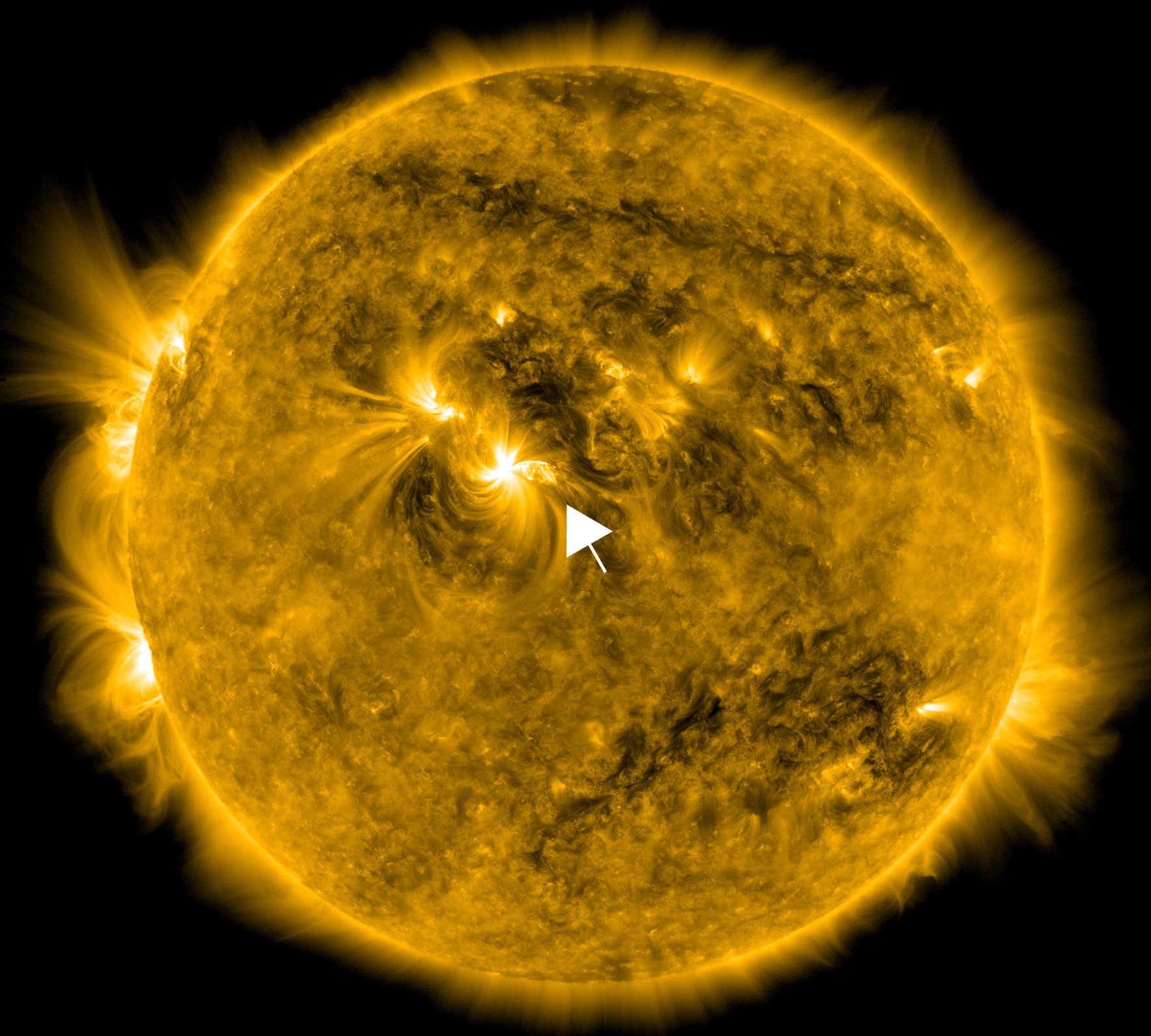
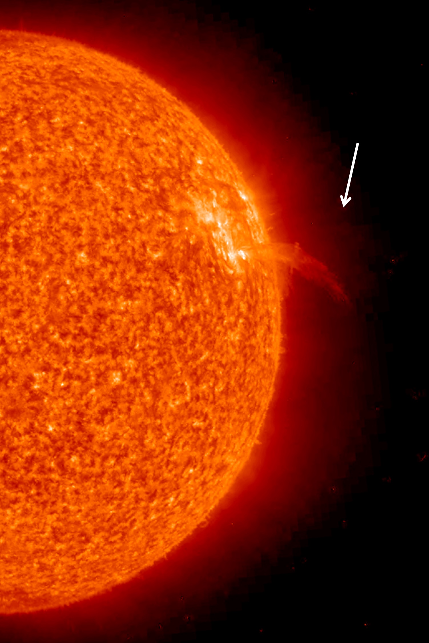
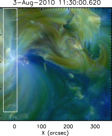
Figure 2 right shows the AR the day after the jet, at the time when the EIS raster named ’D’ was taken. We notice on the west side that the area which had a void and small scale loops has changed and filled by warm loops. We will show in Section 4.3 that some plasma is escaping from this open magnetic field area. The image also shows that the dome structure on the right side of the active region (structure ’B’ in the Figure) is still there after the jet.
On 2 August, some activity in the AR started few hours before the jet. This was in the form of plasma flows and brightening along the loops having the footpoints at the spot in the area labeled ’A’ in Figure 2. During the eruption, the southern part of the jet moved and expanded toward north-west, interacting with the dome-shaped loops system and its spine (arrow ’B’ in the figure). This can also be observed from the vantage point of STEREO EUVI-A and B images, as shown in Figure 1, where the material is released near the limb. In this configuration, STEREO A and B were at separation angles of 71 and 78 degrees, respectively, from the Earth. Due to the location of the jet, the observed opening of field lines, and subsequent release of material, this jet was selected as a good candidate to possibly reach into the heliosphere and be detected by the in–situ instruments.
In the following sections we will describe our attempt to fully understand if this jet material reached the interplanetary medium. We discuss the plasma diagnostics of the AR performed during the period 1-3 August 2010 and the analysis of the magnetic field configuration before and after the jet, at small and large scales. As part of our comprehensive effort to connect the jet, we also modeled the element fractionation within the open and closed regions in order to connect remote sensing and in–situ measurements. We will discuss the search for its signatures within the in–situ measurements in Section 4.7.
3 Methods: Building Blocks for Connectivity
In this section we present the modeling and observational methods used in our attempt to establish the connection between the Sun and the heliosphere and track distinct coronal plasma from its solar origin into interplanetary space. In Sect. 3.1, we review different approaches to modeling the magnetic field in the extended solar atmosphere, including the potential field source surface (PFSS) model, non-linear force free field (NLFFF) modeling, and steady-state magnetohydrodynamic (MHD) modeling. In Sect. 3.2 we present the model for elemental abundance variations. In Sect. 3.3, we review UV spectroscopic techniques and the various plasma diagnostics to determine densities, temperatures, and elemental abundances in the solar atmosphere. In Sect. 3.4, we discuss the in–situ observational techniques for measuring ionic and elemental abundances in the solar wind and the heliospheric back-mapping procedure to estimate their solar origin.
3.1 Modeling the Coronal Magnetic Field Structure
3.1.1 Global PFSS Modeling from Synoptic Line-of-sight GONG and SDO/HMI Magnetograms
The potential field source surface (PFSS) model has been one of the most reliable and robust tools for estimating the large-scale magnetic structure of the solar corona (Altschuler and Newkirk, 1969; Schatten et al., 1969; Hoeksema, 1991; Wang and Sheeley, 1992). In the potential field approximation the magnetic field is derived from
| (1) | |||||
| (2) |
which yields a solution of the form where . The solution is obtained for where the radial field at is taken from photospheric magnetogram observations and the source-surface, , is the distance where the magnetic field is assumed to have become purely radial, typically (Hoeksema et al., 1983). Line-of-sight photospheric observations are used to approximate the radial field at the central meridian with the relation. The scalar potential function can then be solved via a number of techniques and is often represented with a spherical harmonic expansion with the coefficients calculated in the usual fashion from the boundary condition.
While the real solar corona is realistically not current-free, the PFSS model continues to be extremely useful and widely used for estimating the large-scale magnetic field structure of the corona (e.g. Hill, 2018; DeRosa and Barnes, 2018), detailed topological analyses of magnetic flux systems over a wide range of spatial scales (Antiochos et al., 2011; Titov et al., 2011; Scott et al., 2018), for analyzing active region energization (Welsch and Fisher, 2016), as the backbone of semi-empirical solar wind descriptions (Arge et al., 2004), and as inputs for solar and heliospheric MHD modeling (Odstrcil et al., 2004; Tóth et al., 2011; Pomoell and Poedts, 2018) as well as to serve as initial condition for global NLFFF modeling (see section 3.1.2).
In this work, each of the PFSS extrapolations are calculated from their respective magnetogram synoptic maps using the formulas given in Zhao and Hoeksema (1993) for the current-free case. We use a spherical harmonic expansion through degree on the MHD grid (described below) and interpolated to a uniform grid over , , . We have used the standard source surface height of herein, but we note that changing the value can modify the PFSS open flux regions. Several recent studies have investigated this issue when comparing PFSS results with the observed locations and/or sizes of coronal holes (e.g. Linker et al., 2017; Riley et al., 2019; Badman et al., 2020). The results of our PFSS extrapolations are presented in Sect. 4.1.
3.1.2 Global NLFFF Modeling from SDO/HMI Synoptic Vector Magnetograms
The solar corona is considered to be force-free, see Wiegelmann and Sakurai (2012, 2021) for a review. This means that, due to the low plasma in the solar corona, plasma forces can be neglected in lowest order and the Lorentz force vanishes. In this approximation one has to solve the nonlinear force-free field (NLFFF) equations
| (3) | |||||
| (4) |
which we solve in spherical geometry by minimizing the functional:
| (5) | |||||
where the surface integrals contains the observed vector magnetogram , here synoptic vector maps from SDO/HMI (Solar Dynamics Observatory, Helioseismic and Magnetic Imager). We developed an optimization code to minimize the functional (5). As initial condition for the iterative minimization of the functional a PFSS model (see section 3.1.1) is used. The method has been originally proposed in Cartesian geometry by Wheatland et al. (2000). Here we use the spherical optimization code as originally developed in Wiegelmann (2007) and adjusted for the use of synoptic vector maps in Tadesse et al. (2014). As a further refinement we use a 3-level multi-scale approach here to minimize (5). More details on the application of the code to synoptic vector magnetograms and a comparison with other global coronal magnetic field models can be found in Yeates et al. (2018). For our simulations the computational grid is in over the domain , , . The results are presented in Sect. 4.1.
3.1.3 Global Steady-state MHD Modeling
For the global steady-state MHD modeling, we use the Adaptively Refined MHD Solver (ARMS), developed by DeVore and Antiochos (2008) and collaborators. ARMS calculates solutions to the 3D nonlinear, time-dependent MHD equations that describe the evolution and transport of density, momentum, and energy throughout the system, and the evolution of the magnetic field and electric current. The numerical scheme used is a finite-volume, multidimensional flux-corrected transport algorithm (DeVore, 1991). The ARMS code is fully integrated with the adaptive-mesh toolkit PARAMESH (MacNeice et al., 2000), to handle dynamic, solution-adaptive grid refinement and enable efficient multiprocessor parallelization. ARMS has been used to perform a wide variety of numerical simulations of dynamic phenomena in the solar atmosphere, including CME initiation (Karpen et al., 2012; Dahlin et al., 2019; Masson et al., 2019), coronal jets (Pariat et al., 2015; Wyper et al., 2017; Karpen et al., 2017) and interchange reconnection dynamics (Edmondson et al., 2010; Lynch et al., 2014; Edmondson and Lynch, 2017; Higginson et al., 2017a, b; Higginson and Lynch, 2018).
ARMS solves the ideal MHD equations in spherical coordinates,
| (6) | |||||
| (7) | |||||
| (8) | |||||
| (9) |
where all the variables retain their usual meaning, solar gravity is with cm s-2, and we use the ideal gas law . To obtain a basic isothermal solar wind outflow, we set and do not solve the temperature equation. The plasma temperature remains uniform throughout the domain for the duration of the simulation (). The solar wind is initialized in ARMS by first solving the one-dimensional Parker (1958) equation for an isothermal coronal atmosphere,
| (10) |
which is characterized by the base number density , pressure , and temperature . Thus, is the thermal velocity at and the location of the critical point is . The MHD simulation starts with the PFSS initial state for magnetic field everywhere in domain, an initial spherically-symmetric density structure of the form where . We then apply the Parker solution outflow and let MHD system relax toward a quasi steady-state (see description in Lynch et al., 2016). This yields an open–closed magnetic field structure that is more physical than the PFSS extrapolations because of the force balance between the solar wind plasma outflow and the magnetic field tension in the closed flux systems. However, we note that the isothermal condition generates the simplest possible MHD wind scenario, which is done to try to minimize the required computational resources. There are other, more sophisticated thermodynamic MHD treatments that include sources and sinks in the internal energy equation such as thermal conduction, radiative losses, and various coronal heating parameterization (e.g. Lionello et al., 2014; van der Holst et al., 2014; Oran et al., 2017).
For our simulation the isothermal solar atmosphere was initialized with a spherically symmetric density profile with a base density of cm-3, dyn cm-2, and K. This yields a sound speed of km s-1, the critical point of the initial Parker solar wind at , and a solar wind speed at the outer boundary of km s-1. The MHD computational grid utilizes block decomposition in logarithmic spherical coordinates with three levels of refinement above the level 1 grid of blocks over , , and . Each computational block contains cells. The level 3 grid, therefore, represents a resolution in over , , and . The level 4 grid covers the location of the August 02 jet, , , and with an effective resolution of over that region. Results from our MHD modeling are used in Sec. 4.1.
3.2 Modeling the FIP Fractionation and Elemental Composition
A difference in the elemental composition of the solar corona compared to that of the underlying photosphere was first observed by Pottasch (1963). As presented in Section 1, since this first observation, this so-called “FIP Effect” has also been observed in various regimes of the solar wind (e.g. Bochsler, 2007), in solar energetic particles (SEPs) (e.g. Reames, 2018), and in the coronae of other late-type stars (e.g. Drake et al., 1997). The elements that are enhanced are those that are predominantly ionized in the solar chromosphere, which indicates the likely location of the ion neutral separation.
Since the original observation of FIP fractionation, a number of key features of its variation with solar coronal region or solar wind regime have become established, allowing the abundance pattern a certain amount of diagnostic potential. Coronal holes, and the fast solar wind emanating from them, have a relatively small FIP fractionation, by a factor typically of 1.5. Slow solar wind and the closed loop solar corona usually have larger fractionations, as mentioned above by a factor (e.g. Bochsler, 2007). However subtle differences remain. The closed loop solar corona does not show an appreciable fractionation of S, whereas frequently the slow speed solar wind does. The element S (FIP 10.36 eV) is formally a high FIP element, but among high FIP elements has the lowest FIP. This difference also shows up in abundances measured in gradual SEP events compared to those measured in accelerated particles in co-rotating interaction regions (Reames, 2018), with the implication that seed particles for shock acceleration in gradual SEP events originate in the solar corona, whereas those for particle acceleration in co-rotating interaction regions are swept directly out of the ambient solar wind.
Further variations in fractionation are also seen in the coronae of active stars, and more recently in some solar flares, where the FIP effect is inverted. This depletion of the low-FIP element abundances has become known as the Inverse FIP or I-FIP Effect, and posed a particular challenge to understanding the phenomenon. While various mechanisms might be able, qualitatively at least, to accelerate chromospheric ions into the corona in preference to chromospheric neutrals, the reverse is more difficult to envisage. One mechanism of fractionation that does offer the possibility to act in either direction, and which also captures the variations in fractionation outlined above is that due to the ponderomotive force (e.g. Laming, 2004b, 2009, 2012, 2015). This arises due to the effects of wave reflection and refraction as Alfvén waves propagate through the chromosphere. The chromospheric wave field depends on the coronal magnetic field structure above it, hence the difference between open and closed fields, but the fractionation also depends on local chromospheric physics.
The instantaneous ponderomotive acceleration, , acting on an ion is evaluated from the general form (see e.g. the appendix of Laming, 2017)
| (11) |
where is the wave (transverse) electric field, the ambient (longitudinal) magnetic field, the speed of light, and is a coordinate along the magnetic field.
Given the ponderomotive acceleration, element fractionation is calculated using input from the chromospheric model (Laming, 2017)
| (12) | |||||
This equation is derived from the momentum equations for ions and neutrals in a background of protons and neutral hydrogen. Here is the element ionization fraction, the element atomic mass number, and are collision frequencies of ions and neutrals with the background gas (mainly hydrogen and protons, given by formulae in Laming, 2004b), represents twice the square of the element thermal velocity along the -direction, is the upward flow speed and a longitudinal oscillatory speed, corresponding to upward and downward propagating sound waves. At the top of the chromosphere where background H is becoming ionized , and small departures of from unity can result in significant decreases in the fractionation. This feature is important in inhibiting the abundance enhancements of S and P at the top of the chromosphere (Laming et al., 2019). These are the high-FIP elements with the lowest FIP (10.36 and 10.49 eV respectively) and reach high levels of ionization () in this region. Lower down where the H is neutral this inequality does not hold, and these elements can become fractionated. Results from this model are presented in Section 4.6.
3.3 Coronal Observations and EUV Plasma Diagnostics
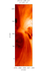
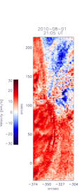
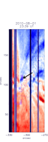
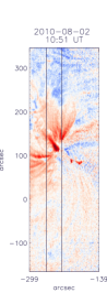
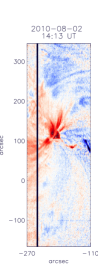
The solar conditions for the three days period of interest were investigated using Hinode/EIS (EUV imaging spectrometer) UV data (Culhane et al., 2007). Several observations are summarized in Table 1. The EIS studies had different properties but they were mostly centered in the spot, as shown in Figures 2, 7, 8 and 9.
For 1 August, the analysis of two different datasets has provided a quite complete picture of the pre-eruption AR conditions. In particular, a full-spectrum (dataset B) has been used for the FIP bias diagnostics. The dataset taken on 2 August (dataset C), contains a very limited number of lines which could only be used for Doppler maps in Fe XII. These, however, provide us with temporal information. Density and Doppler maps could be obtained also for 3 August (dataset D).
The EIS data have been processed using the standard software available on the EIS database, unless differently stated. The spectral line profiles and total intensities were measured assuming a Gaussian profile using the Del Zanna (2013) radiometric calibration.
The plasma diagnostics were done using the CHIANTI v.8 atomic and software database (Dere et al., 1997, 2019), unless differently mentioned. Synthetic line intensities were calculated assuming ionization equilibrium and photospheric composition (Asplund et al., 2009). Density maps of the observed regions were obtained applying the line ratio technique to Fe xiii (Parenti, 2015) diagnostics (see Section 4.4). The Differential Emission Measure distribution (DEM) was derived using the (Del Zanna, 1999) method which provides the thermal structure distribution of the plasma integrated along the line of sight. The FIP bias analysis was done using two different methods: the DEM and LCR (see Sections 4.4.1, 4.4.2).
| Inst. | Date | Start | End | Set | Center | FOV |
|---|---|---|---|---|---|---|
| [UT] | [UT] | [x′′, ] | [, ] | |||
| EIS | 1/8/2010 | 21:05:24 | 21:15:05 | A | -337.8, 94.3 | 69.9, 248.0 |
| EIS | 1/8/2010 | 23:39:35 | 00:41:28 | B | -315, 93.3 | 60.0, 512.0 |
| EIS | 2/8/2010 | 10:51:02 | 11:36:08 | C | -219.3, 90.0 | 159.7,512.0 |
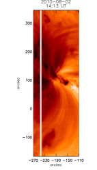
| EIS | 2/8/2010 | 14:13:01 | 14:58:06 | C | -189.8, 89 | 159.7, 512.0 |
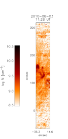
| EIS | 3/8/2010 | 11:28:21 | 11:46:44 | D | -16.5, 106.2 | 50.9, 384.0 |
3.4 Connecting Solar to the in–situ Observations
In this section we describe the technique we used for another important block for our Heliophere-Sun connectivity, that is the procedure which backs-map the in–situ measures to a location on the solar surface.
The heliospheric structure of the solar wind’s Parker spiral (Parker, 1958) can be estimated through integrating the velocity streamlines associated with the observed radial speed measurements at 1 AU. Assuming the observed radial speed is constant, this yields
| (13) | |||||
| (14) |
where the solar rotation rate rad s-1. This ballistic back-mapping projects the time series of plasma observed at 1 AU (which has an equivalent longitude in each Carrington Rotation) backwards in time to an earlier radial location, taken here to the be potential field source surface at . The resulting Carrington longitude of the velocity streamline origin has an equivalent date and time corresponding to the time the plasma parcel was released from the Sun. From the inner boundary of the ballistic back-mapping, a coronal magnetic field model or extrapolation (e.g. PFSS, NLFFF, MHD) can then be used to continue the mapping from the corona to the solar surface. This ballistic mapping method has been applied to Ulysses data and discussed by Neugebauer et al. (2002, 2004) and variations of this approach continue to be used to analyze solar wind source regions (e.g. Gibson et al., 2011; Zhao et al., 2013a, b, 2017a; Badman et al., 2020). Note that the overall uncertainty in the position of the footpoint of the magnetic field lines as mapped by these techniques are within approximately 10∘ (Neugebauer et al., 2002; Leamon and McIntosh, 2009). Results for this analysis are given in Section 4.7.
4 Results
4.1 Global Magnetic Field Configuration for 2010 August 02
We apply each of the magnetic field modeling techniques described in Section 3.1 to various synoptic magnetogram data during Carrington Rotation 2099 (observed from 13 July through 08 August) which encompasses the 2010 August 02 coronal jet. Figure 3 shows the results of the global PFSS, NLFFF magnetic extrapolations and steady-state MHD modeling, co-aligned such that August 02 (yellow dashed line) corresponds to a Carrington Longitude of in each panel.
The top panel of Figure 3(a) shows the GONG synoptic map111ftp://gong2.nso.edu/oQR/zqs/201008/mrzqs100802/mrzqs100802t1154c2099_034.fits.gz interpolated to a uniform grid in . The bottom panel of Figure 3(a) plots the open field footpoints in green (positive polarity) and red (negative polarity) along with the global helmet streamer structure (blue field lines) and the neutral line at representing the cusp of the global helmet streamer belt. Figure 3(b) shows the HMI radial field synoptic map222http://jsoc.stanford.edu/data/hmi/synoptic/hmi.Synoptic_Mr_small.2099.fits on a grid and the corresponding open field regions and streamer belt configuration. Figure 3(c) shows the results for the global, spherical NLFFF modeling (3.1.2) based on the HMI synoptic vector magnetograms333for an overview http://hmi.stanford.edu/hminuggets/?p=1689 for CR 2099. Here, the upper panel shows the NLFFF solution at (rather than the observed synoptic map), and the lower panel plots the open field foot points colored by their polarity, representative streamer belt field lines, and the contour at as the black line to indicate the streamer cusp and heliospheric current sheet location. Figure 3(d) shows the steady state MHD solar wind outflow (3.1.3) based on the GONG PFSS magnetic field extrapolation for the initial magnetic state using degrees of the spherical harmonic expansion. As in panel (c), the top panel shows the PFSS solution at , and the bottom panel shows the open field regions and streamer structure at hr into the solar wind relaxation.
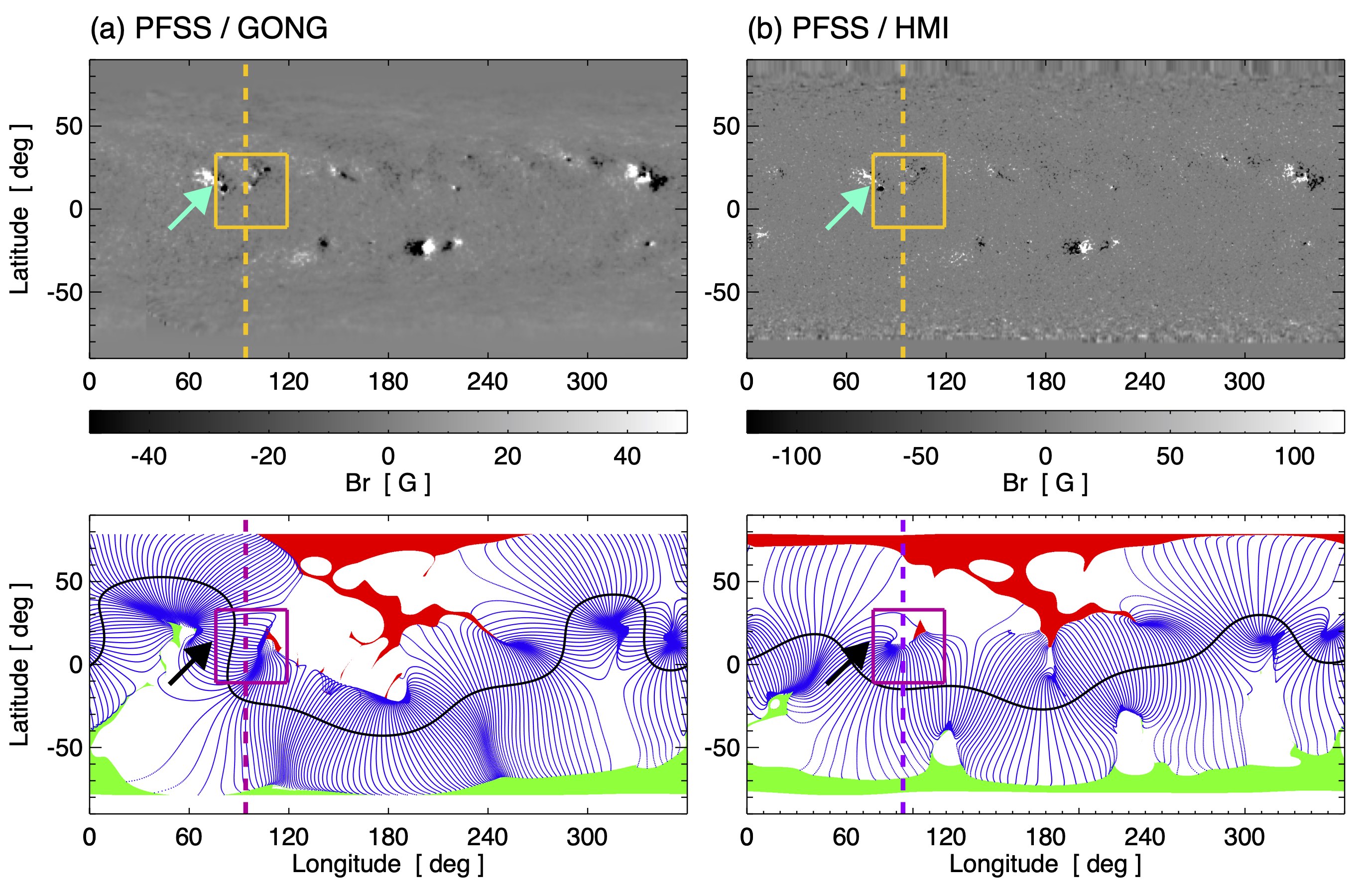
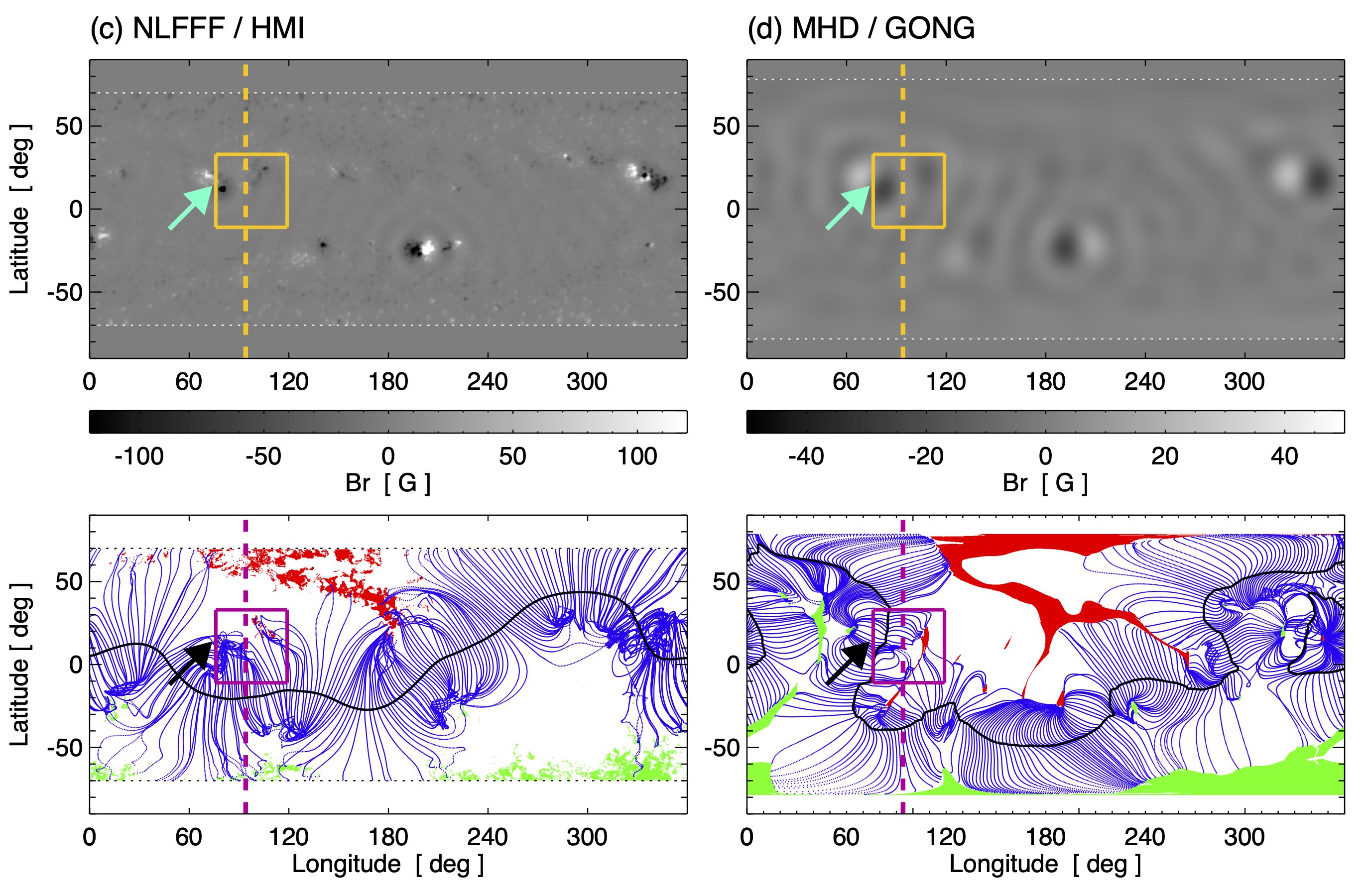
Figure 3 illustrates both similarities and differences in each of the global magnetic field models. In a rough, qualitative sense, the open field regions of the large-scale coronal holes are essentially in agreement. The northern negative polarity coronal hole has an extended “elephant trunk” structure extending to low-latitudes and the global helmet streamer belt shape has significant excursions above and below the ecliptic plane, as characterized the contour at 2.5 in black and the spatial coverage of the blue streamer belt field lines. While the GONG-based modelling shows the helmet streamer belt extending to greater latitudes than the HMI-based modelling, in general, both the NLFFF results (based on HMI synoptic map show) and the steady-state MHD results (based on the GONG synoptic map) maintain their qualitative agreement to the global configurations of the PFSS extrapolations based on their respective source synoptic maps. We note that the PFSS/GONG extrapolation does not capture the open field region adjacent to AR 11092 that is present in both of the HMI-based models at a Carrington longitude of 84∘ just west of the arrow (see also Figure 5). However, the MHD configuration does recover this AR-adjacent open field due to the restructuring of the open-closed flux boundary and establishment of the force-balance of the steady-state solar wind outflow.
A quantitative characterization of the differences in the modelling results is presented in Table 2 where we compare properties of the global magnetic field distribution in each of the model cases. The four columns represent each of the models shown in Figure 3. The first three rows are the minimum and maximum ranges of on the lower boundary, followed by the total unsigned radial magnetic flux, , at radial heights of , and the total magnetic energy . For the MHD simulation, the radial fluxes and total magnetic energy values are at hr, i.e. at the end of the steady-state solar wind relaxation. The differences in between and show the same level of variation seen between the different models. The fact that three of our four cases have regions of open flux adjacent to our jet event location ensures this is a robust feature of the large-scale topology. We also refer the reader to the study by Riley et al. (2019) that examines the impact of varying the PFSS source surface height on the area and shape of open flux regions.
| PFSS (GONG) | PFSS (HMI) | NLFFF (HMI) | MHD (GONG) | |
| [G] | ||||
| [G] | ||||
| [G] | ||||
| [Mx] | ||||
| [Mx] | ||||
| [Mx] | ||||
| [Mx] | ||||
| [erg] |
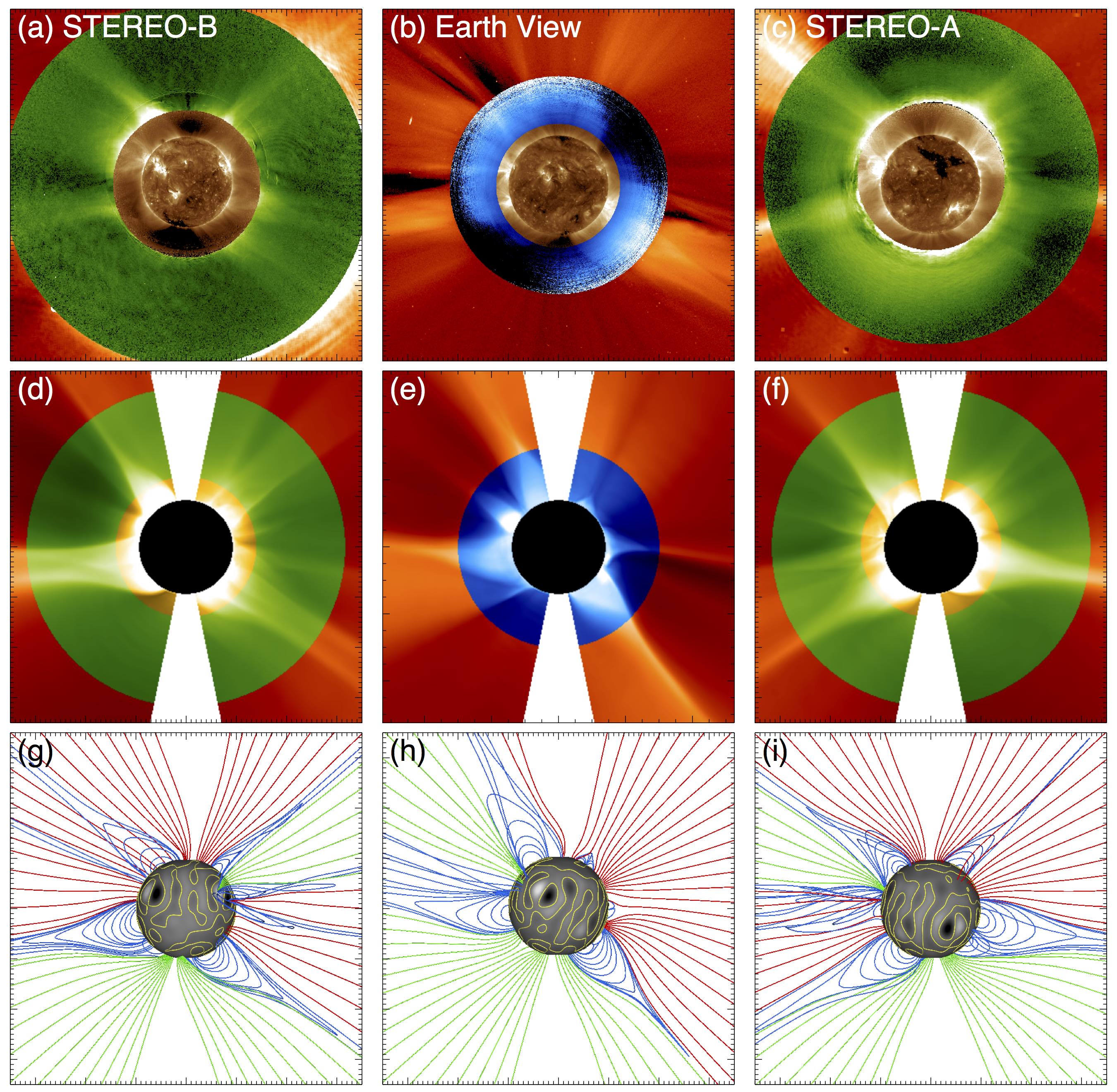
Figure 4 presents the comparison between the multi-viewpoint white-light coronagraph observations with the steady-state MHD wind outflow and its resulting streamer structure shown in Figure 3(d). The top row of Figure 4 contains the (a) STEREO-B, (b) Earth view, and (c) STEREO-A perspectives as composite plots of EUVI, COR1, and COR2 data in panels (a) and (c), and a composite plot of AIA, the HAO MLSO MK4, and LASCO C2 data in panel (b). The middle row of Figure 4, panels (d)–(f), show the synthetic white light intensity derived from the MHD 3D density data cube, normalized by the hr spherically-symmetric density profile (as in Lynch et al., 2016). The bottom row of Figure 4, panels (g)–(i), show the representative open field lines colored with the same positive, negative (green, red) polarity and the closed field streamer structures (blue) in the plane of the sky for each respective viewpoint.
The qualitative agreement between the observed and modelled helmet streamer structure is quite reasonable. The MHD simulation’s synthetic brightness structures (corresponding to the line-of-sight integrated white light emission from the density enhancements of the global helmet streamer belt and the largest pseudostreamers) occur at approximately the same locations with approximate the same widths as the observed coronagraph features. The agreement for the STEREO spacecraft viewpoints is a bit better than the LASCO/Earth-view. In general, the disagreement is most apparent in the simulation streamers being slightly more radial than the observed streamers. This is influenced by the nearby open field strengths and their resulting open fluxes. The representative open field lines of Panels (g)–(i) were traced from a series of points in the selected planes-of-the-sky so some overlap between these open field lines and some of the representative closed streamer field lines (blue) show that there are significant line-of-sight contributions in both the observed and synthetic white-light intensities.
4.2 Local Magnetic Field Configuration for 2010 August 02
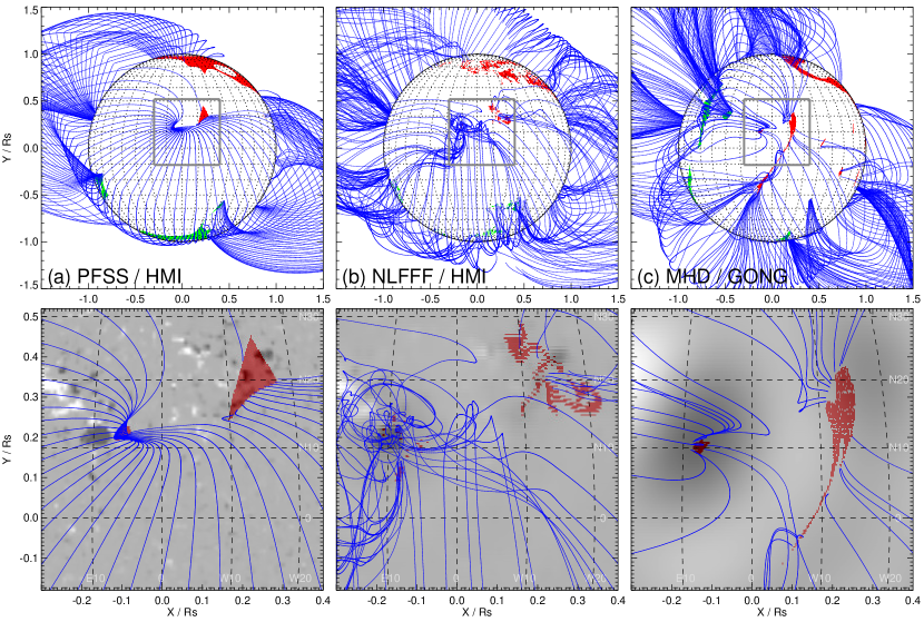
In this section, we further examine the coronal magnetic field structure in the vicinity of AR 11092 and the August 02 jet source region in order to investigate the relationship between these structures and the EUV remote sensing observations of the coronal plasma. The top row of Figure 5 plots the Earth-view of the large-scale coronal topology associated with the helmet streamer belt (blue field lines) and the (positive, negative) open field regions (green, red) predicted from the (a) PFSS/HMI, (b) NLFFF/HMI, and (c) steady-state MHD/GONG modeling results presented in Figure 3. In each panel, we have drawn a box on the disk face corresponding to the approximate field-of-view of the region encompassing the various EUV spectroscopy measurements. The bottom row of Figure 5 plots each of the regions indicated above ( 670”670”) including the strong-field negative polarity spot in AR 11092 and the AR-adjacent open field regions (red shading).
There are both similarities and differences in each of the magnetic field modelling results in and around the coronal jet source region. Each model produces some small concentration of open flux associated with the western edge of AR 11092 and larger region of open flux further west, even in the PFSS and MHD cases where the magnetic field on the 1 boundary is severely under-resolved. Based on the visual inspection, the shapes of these open flux concentrations are quite different, but their overall locations with respect to AR 11092 are in fairly good agreement. The helmet streamer field lines are representative of the open-closed field topological boundary. Additionally, in each case, the two concentrations of negative polarity open fields signify a pseudostreamer-like closed-flux system to the west of AR 11092. This recalls the dome structure visible in Figure 2 label as ’B’. For the purposes of our investigation herein, the fact that each model reproduces open flux in the immediate vicinity of the observed AR jet means that there is a strong possibility for at least some AR material to end up on open or newly-opened field lines during the eruption process.
4.3 Local Magnetic Field Configuration for the Period August 1–3
We inferred the temporal evolution of the magnetic field around the spot during the period August 1–3 applying the NLFFF method described in Sec. 3.1.2. Differently from what made for the global extrapolation in the previous section, here we used the daily vector magnetic field data. This would be a more representative for the temporal evolution of the smaller scale features.
We used full disk vector field for the 1st, 2nd and 3rd of August 2010 obtained in Heliographic–Helioprojective Cartesian (HGLN/HGLT-HPC). All the vector magnetic field data are provided by SDO/HMI. The computational grid is 256x372x512 over the domain r/R⊙ [1, 2.5], [20∘, 160∘], [90∘, 270∘].
We applied the NLFFF model on HMI data before the jet on 1st of August 2010 at 23:36:00 UT, 2nd of August at 14:12:00 UT and after the jet on 3rd of August at 11:48:00 UT. From the solution of the extrapolation we trace the open field lines from the photosphere into the corona at 2.5 which we display in Fig. 6, left column. We performed the tracing of the field lines for window of 7∘ latitude and 10∘ longitude, around the sunspot. We also traced in back the field lines rooted in the CO1 region. While the position of the latitude window remains the same in all of the images, the position of the longitude window changes with the solar rotation.
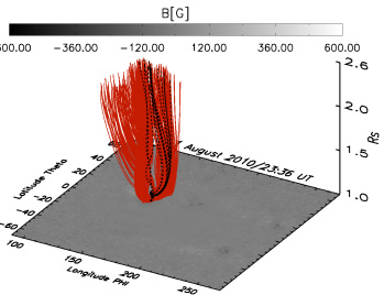
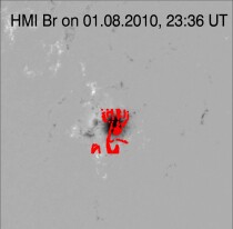
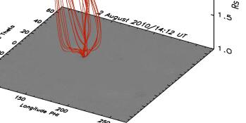
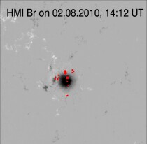
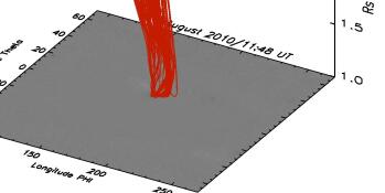
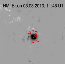
In Fig. 6 right column we show the photospheric footprints of the open magnetic field lines overplotted over the HMI radial magnetic field. The variations in the local topology of the magnetic field are strongly visible before and after the jet. We remark a decrease of open field before the jet, probably connected with the activity visible in the SDO/AIA data in the region before the jet and indicating that some reconnection have already taken place. Our results also show a variation of the volume occupied by this open field with different expansion with height during the three days. Some small differences in the position of the open field footpoints for the 2nd of August is visible between this result and that shown on the middle panel of Figure 5. But the general agreement that the area around the spot contains open flux tubes is respected.
4.4 Corona plasma parameters from EUV observations.
Using the datasets listed in Table 1 we performed the diagnostics analysis for density, temperature, Doppler motion and FIP bias in various area of the active region. Our purpose is to identify any difference within the active region that can uniquely be used to possibly match the interplanetary properties measured by WIND at the estimated solar wind arrival time.
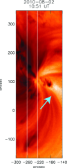
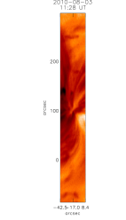
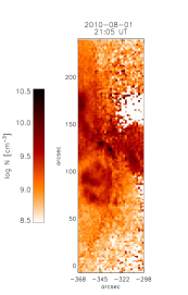
The top line and middle panel of the bottom line of Figure 7 show the Fe xii 195.2 Å intensity (negative) maps for the rasters listed in Table 1, A, C and D. We can identify the spot at the center of the FOV and the long loops in the middle-left side of it. The south-west side of the rasters is the area interested by the jet eruption. This indeed is the area where we see the highest topological change from August 1st to the 3rd. These different structures of the AR will be investigated in Section 4.4.1. The first and third panels of the bottom line of the figure show the density maps for the 1st and 3rd of August respectively, and are obtained from the line ratio technique applied to the Fe xii 186.8/195.12 Å lines. These maps are quite noisy, but we clearly see the morphological change of the denser core of the AR. When comparing the intensity map for the 2nd of August with Fig. 5, we see consistency in the morphology with both zoomed panels (a) and (b), even though panel (b) shows the open channel and more complex field distribution in the jet location.
|
|
4.4.1 Pre-eruption AR from the EIS full spectrum on August 1st
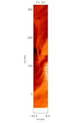
On August 1st EIS rastered the jet region with the 1" slit in about 1 hour. It recordered the full spectrum (dataset B in Table 1). Figure 8 shows SDO/AIA images of the AR on August 1st, with the FOV of the full EIS raster superimposed. The observation was about 17 hours before the jets observed on August 2nd. The EIS FOV was centred on the western sunspot region. The AIA 195 and 335 Å images, dominated by 1.5–3 MK plasma (Fe xii – Fe xvi) in the AR core, show the ’dark’ channel, site of coronal outflows and the jet evolution (see also Figure 2, arrow ’C’).
The AIA 171 Å shows 1 MK plasma (Fe ix). It is clear that a fan system of cool loops extending towards the west is superimposed on the coronal outflow channel. Various other system of loops extending towards the east are the brightest features in the image. Finally, the usual dark channel is clearly visible as surrounding the AR core.
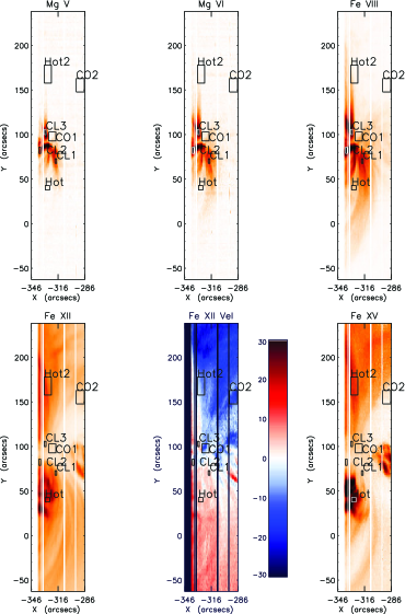
The black box in Figure 8 shows the inner region of the EIS FOV, displayed in Figure 9, which shows the intensities in a selection of spectral lines, as well as the Doppler image in Fe xii. The EIS data were processed using custom-written software by one of the authors (GDZ) which essentially reproduce the steps in the t routines, with the difference that bad pixels are replaced with interpolated values and the pseudo-continuum (bias) is removed when fitting the spectral lines. The Doppler image was obtained by removing the orbital variations and the expected variations along the slit, as described in the EIS software note No. 23. For the rest wavelength, we used a region in the bottom of the slit, outside from the FOV in the image, and from the AR core. The EIS spectra are dramatically different depending on the source region. Despite the 60s exposures, spectra needed to be averaged over some regions, especially where the coronal signal is low. The regions selected for further analysis are shown in Figure 9. ‘CO1’ is the main region, close to the Sunspot and the origin of the jet, within a coronal outflow region (blueshift in the Doppler map). ‘CO2’ is a similar region. ‘Hot’ and ‘Hot2’ are two regions with strong emission around 3 MK, and little emission at lower temperatures. ‘Hot’ is on a system of short loops, while ‘Hot2’ is on a system of long loops. Finally, three regions on the cool loops extending towards the west were selected (CL1, CL2, CL3). Again, the loops have different lengths. Little hotter emission is present along the line of sight.
We obtained averaged spectra and carefully fitted all the lines. The most important lines for chemical abundance diagnostics are very weak. We then performed a DEM analysis (Del Zanna, 1999) to obtain the temperature distribution and the relative chemical abundances, using CHIANTI version 8 atomic data (Del Zanna et al., 2015) although we note that changes in the latest version 10 only introduce small (10–20%) differences in a few ions. We used a constant density of 2109 cm-3 for all the regions (consistently with the values found by applying the line ratio technique in Section 4.4, Figure 7) to calculate the contribution functions of the lines.
An example is shown in Figure 10, for the coronal outflow region CO1. The points indicate the ratio of the predicted vs. observed radiance, multiplied by the DEM value at an effective temperature (i.e. an average temperature weighted by the DEM distribution). The emission in the 2–3 MK region is an order of magnitude lower than the typical emission in active regions. The FIP effect can only be constrained by the Fe /S relative abundance. Lines from S viii, S x, S xiii were clearly observed. There are plenty of strong Fe lines to constrain the DEM. The coronal abundances discussed in Del Zanna and Mason (2018), where Fe /S is enhanced by a factor of 3.2 over its photospheric value (Asplund et al., 2009), were used. Ar xiv is at the limit of detectability, which further confirms that the abundances were not close to photospheric, otherwise the high-FIP Ar line would have been much stronger and easily observed. The weak Ar emission is consistent with this FIP effect of 3.2. Note that the emission in the coronal outflow region is strongly multi-thermal. Also note that the peak of the DEM, at much lower temperatures, refers to the cool fan loops along the line of sight that are clearly visible in the EIS Fe viii (and in the AIA 171 Å image, which we have mentioned).
Other coronal outflow regions such as CO2 showed the same coronal abundances. The hot loop regions also had the same abundances, in agreement with the AR core results reviewed by Del Zanna and Mason (2018). In this case, additional lines from S xi and S xii could be used.

On the other hand, all the cool loop legs (CL1, CL2, CL3) indicated a much smaller FIP effect, with abundances closer to the photospheric values of (Asplund et al., 2009). The DEM is well constrained by several strong lines from low FIP ions: Mg v Mg V, Mg vi, Mg vii, Si vi, Si vii, and Fe viii. The available high-FIP ions are O v and O vi only. Using the CHIANTI v.8 ionization equilibrium we obtain relatively good agreement between O v, O vi and the low-FIP lines with an FIP bias of 1.8, for CL1 and CL3. For CL2, the intensities of the O v lines are consistent with photospheric abundances, while those of O vi are consistent with an FIP bias of 1.6. As O vi is one of the ‘anomalous’ ions, where typically predicted intensities in the quiet Sun are a factor 3-5 lower than observed (Del Zanna and Mason, 2018), we think that the O v results are more reliable. Density-dependent effects in the ionization equilibrium are known to improve predictions. For a recent example on the quiet Sun, see Parenti et al. (2019), and for recent calculations on C and O ions Dufresne and Del Zanna (see 2019) and Dufresne et al. (2020). Such effects are also taken into account within ADAS444https://www.adas.ac.uk; https://open.adas.ac.uk (Atomic Data and Analysis Structure, see, e.g. Summers et al. (2006); Giunta et al. (2015)), which deals with a full density dependent collisional-radiative modelling applied to astrophysical and controlled fusion plasmas. As significant uncertainties in the ion abundances are present for some of the elements considered here, we have not included these effects, which in general tend to shift the temperature of formation of these ions to lower temperatures, but do not affect significantly the relative abundances. The main uncertainties are in the EIS relative calibration and in the ionization equilibrium. They are not simple to estimate, but are of the order of 30%. The summary of our results for the FIP bias are listed in Table 4 bottom line.
4.4.2 Estimating the FIP bias using an alternative diagnostic method
In addition to the previous analysis, we determined relative FIP bias maps for these regions of interest at four different temperature ranges using the linear combination ratio (LCR) method (Zambrana Prado and Buchlin, 2019). This method allows us to determine relative FIP biases in the corona from spectroscopic observations in a way that is in practice independent from DEM inversions. We optimize linear combinations of spectral lines of low-FIP and high-FIP elements so that the ratio of the corresponding linear combinations of radiances yields the relative FIP bias with a good accuracy. We developed a Python module, which is available at fiplcr, to compute the optimal linear combinations of spectral lines and to use them to compute relative FIP bias maps from observations. The CHIANTI database version 9.0 was used together with the ChiantiPy Python package (version 0.8.5), although we note that the data for the coronal ions is the same as in version 8. To perform the optimisations we used contribution functions computed with the same density as the previous analysis (), and we computed the relative FIP biases using the radiances previously obtained. We used three sets of spectral lines that were observable in all regions and a fourth set that was observable only in regions CO1 and CO2; they are listed in Table 3. We determine either the iron to sulfur Fe /S relative abundance, a mix between silicon and iron to sulfur (Fe & Si)/S, or a mix between calcium and iron to argon (Ca & Fe)/Ar.
| Set # | Ion | Wavelength | FIP | |
| (Å) | (K) | (eV) | ||
| 1 | S viii | high (10.36) | ||
| Si vii | low (8.15) | |||
| Si viii | low | |||
| Fe x | low (7.9) | |||
| Fe xi | low | |||
| 2 | S x | high | ||
| Si x | low | |||
| Fe xiii | low | |||
| Fe xiv | low | |||
| 3 | S xii | high | ||
| S xiii | high | |||
| Fe xv | low | |||
| Fe xiv | low | |||
| Fe xvi | low | |||
| 4 | Ar xiv | high (15.8) | ||
| Ca xiv | low (6.11) | |||
| Fe xv | low |
The results from the FIP bias measurements at different temperatures are given in Table 4. We assumed photospheric abundances from Asplund et al. (2009). The relative FIP bias value obtained is listed for every selected region. The uncertainties are computed using a statistical approach based on the Bayes theorem555We use Monte-Carlo simulations to simulate noisy radiances by adding Gaussian random perturbations with a 20% standard deviation assuming that this would be a typical error bar one would obtain for the radiances of EIS observations. From these noisy observations computed assuming different relative FIP biases we obtain , the probability distribution of the real relative FIP bias of the plasma knowing that we have obtained a measured (inferred) relative FIP bias .. It allows us to define the likelihood of the plasma’s real relative FIP bias given the inferred relative FIP bias measured with spectroscopic observations. Using this probability distribution we compute the credibility interval at 75% which is also listed for every measurement in Table. 4.
Sulfur is an intermediate FIP element which can be subject to a slight enhancement of its abundance. It is therefore no surprise that we obtain a higher value when comparing iron and calcium to argon in set #4, argon having a much higher FIP than sulfur. In the CO1 and CO2 regions we observe an enhancement of low FIP elements as compared to sulfur of a factor 2 and at least a factor 3 when compared to argon. We should however note that the argon and calcium lines are very weak. As we have used Gaussian noise with a standard deviation of 20% to simulate noise for all lines, the uncertainties for the relative FIP bias obtained are most likely underestimated as these very weak lines (at least an order of magnitude lower than the iron line we also have in this set) would drag along more noise. The hotter loop regions HOT and HOT2 show photospheric abundances at lower temperatures (results of set # 1). Given that the very hot loops we wanted to analyse within this region barely exist at those temperatures and that coronal plasma is optically thin, what we are seeing in this temperature range is probably the underlying quiet sun material which does generally have abundances closer to photospheric. Higher in temperature we see an enhancement in the abundance of low FIP elements closer to a factor 2. We find similar results to the DEM analysis (Section 4.4.1) for regions CO1 and CO2. Concerning the hot loops, the LCR method yields lower abundance biases, still consistent with the DEM analysis.
| Set | CL1 | CL2 | CL3 | CO1 | CO2 | HOT | HOT2 |
|---|---|---|---|---|---|---|---|
| 1 | |||||||
| 2 | |||||||
| 3 | |||||||
| 4 | |||||||
| B |
4.4.3 Evolution of the AR between 1 and 3 August
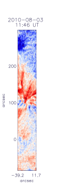
Figure 11 second panel shows a zoom of the velocity map of Figure 9. The other panels shows the maps of Doppler shift in the range for the A, C and D rasters (1st, 2nd and 3rd August) derived from Fe xii. The reference position of the line was obtained as follow. For each spatial pixel the line profile was fitted using a double-Gaussian as suggested by Young et al. (2009). The position of the brightest component of the Fe xii doublet was averaged (in the post-processed data, that is applying the correction for orbital variation and variations along the slit) in a QS region within the raster. We do not have an appropriate QS area, however, we did this for the datasets C and D, selecting a box of 20 pixels in the bottom of the raster. For the dataset A we adopted as reference the averaged line position within the whole raster (Peter and Judge, 1999).
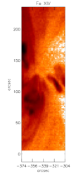
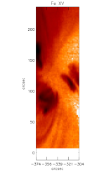
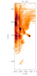
In the second velocity map in Figure 11 have overplotted in violet the open magnetic field lines footpoints obtained from the NLFFF extrapolation. We see that the outflow ’CO1’ region is consistent with the open flux located close to the spot. The first panel in the figure is the map obtained from the data taken two hours earlier than the second panel (and which has a slightly different FOV). The two maps are similar even though the lower exposure time of the first dataset makes the map noisier. The small outflow region (CO1 is part of it) on the north part of the spot is still present. The larger upflow areas on the top of the raster are possibly associated with the quasi-horizontal loops (as projection effect) that are better visible in the third and fourth panels (see also Figure 7 and Figure 1). The third and fourth panels (2nd August) show some red-shift spots associated with the jet precursor activity along the jet channel. These may be the signatures of flows due to reconnection events. In this respect we also plot in Figure 12 intensity maps for the hotter Fe xiv– xv (depending on the available lines in the data) during the three days. We see the hot core of the AR with short loops on the 1st of August (first two panels). On the 2 August we clearly see an hot blob in the jet channel in correspondence of the red-shifted blob of Figure 11, panels 3 and 4. We remind that these data are taken few hours before the jet. On the day of the jet and afterward, the north part of the spot becomes completely red-shifted and loop-shaped.
|
|
4.5 Linking the results from EUV data with the modelling
In this section we examine the MHD simulation results in the context of the EUV observations and discuss the quantities from the global modelling that are provided as inputs to the more detailed FIP modelling in Sect. 4.6. Figure 13 displays several magnetic field and plasma properties of the MHD solution in the vicinity of the AR jet, i.e. in the same viewpoint shown in Figure 5.
In Figure 13(a), we show the flux tube expansion factor (Wang and Sheeley, 1990), calculated as , where the starting foot point of each magnetic field line (flux tube) is given by . We construct a uniform grid in for the field line foot points on the lower boundary, with and . For the field line geometric quantities in this section, we use the near-Sun portion of the global domain, , i.e., if the field line passes through the surface, we consider it “open.” The expansion factors for closed field lines are calculated in exactly the same way. However, since for closed field lines, only the ratio contributes to . The geometry of the open-field magnetic flux tubes are a key parameter in both semi-empirical models of the solar wind (e.g. the Wang-Sheeley-Arge model; Arge et al., 2004; Wang, 2012) and the more sophisticated, first-principles 1D calculations (e.g. Hansteen and Velli, 2012; Cranmer, 2012; Pinto and Rouillard, 2017). Likewise, the field line length of closed flux tubes constrain the low-frequency input (and available resonances) for waves and turbulence in these loops and therefore is an important component of the FIP fractionation modeling based on the wave interactions at the corona-chromosphere transition layer.
The open magnetic field regions are indicated with the cyan/blue contours in each panel. In Figure 13(a), we see that the largest expansion factors () are clearly associated with the regions of open field. The presence of open field around the spot area is confirmed by the results from the PFSS and NLFFF models shown in Figures 5(a),(b), 6, which use HMI magnetograms or synoptic maps, as well as the MHD model using the NSO/GONG synoptic map (Figures 5(c)).
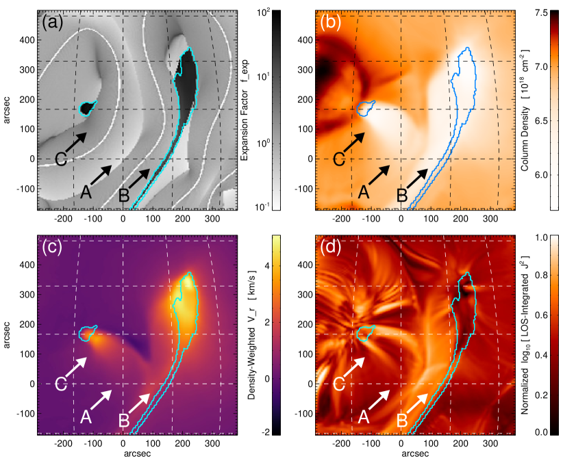
Figure 13(b) plots the column number density, , where we approximate the line-of-sight integral as along the radial direction and take . For panels 13(b) and (c) the range of the radial line-of-sight was in order to highlight the low-coronal structure. For panel 13(d) the radial line-of-sight was to minimize the contribution of the lower boundary current structure. Figure 13(c) shows the line-of-sight integrated, density-weighted radial velocity, given by , where the weights are defined as the normalized density distribution with height .
The density map of panel (b) can be qualitatively compared to the AR density around the spot shown in the first panel of the second row of Fig. 7, obtained from about 1MK plasma emission data of the 1st of August. The east denser structures are there, while the less dense jet channel in the model is replaced in the data by a much more dense short loops structure. We know that the latter will be modified and reduced prior and after the jet (see also Figure 2) leaving the space to the more ’empty’ jet channel.
The velocity map in figure (c) cannot be quantitatively compared with the velocity maps from the data, as the latter are LOS averaged values. However, it is interesting to see that the model identifies an outflow area in the jet channel similarly to the data (see Fig. 9 panel 5 and Fig. 11).
Figure 13(d) shows a synthetic EUV emission formulation that is a simplified version of the Cheung and DeRosa (2012) electric current density-based emission proxy. Here we use , which avoids averaging over a field-line for every point along the radial line of sight. The Cheung and DeRosa (2012) current-based emission proxy has been favorably compared to the morphology of AIA 131Å (see also Hoeksema et al., 2020), and here it shows more qualitative agreement with our hottest lines, specifically Fe xiv– xv (formed around 1.5 – 2.5 MK, see Fig. 12).
4.6 Modelling the FIP bias
The modelling described above allows us to identify magnetic field strengths associated with the various regions singled out for spectroscopic analysis, and use this information to calculate expected FIP fractionations. We first consider the closed field regions, CL1, CL2, and CL3 on Figure 9. We assume that the FIP fractionation in closed loops is caused by Alfvén waves generated in the corona (Laming, 2017), presumably by nanoflare reconnection events. This provides a rationale for having waves resonant with the loop, where the wave travel time from one loop footpoint to the other is equal to an integral number of wave half periods. In such a case, fractionation by the ponderomotive force is restricted to the top of the chromosphere where H is becoming ionized. Moving low FIP ions through a background of protons requires a strong ponderomotive force, and even a small neutral fraction can diffuse back down the concentration gradient eliminating any fractions. Consequently elements have to be almost completely ionized to fractionate, and intermediate elements like S behave much more as high FIP elements. This leads to significant fractionation in e.g. the Fe /S abundance ratio.
A further consideration for waves of coronal origin from nanoflares is that the Alfvén speed be sufficiently high. This means that waves from a reconnection event can reach the chromosphere and cause fractionation before the heat conduction front arrives to evaporate the chromospheric plasma up into the corona. The simplest (possibly naive) criterion for FIP fractionation should then be that the coronal Alfvén speed being higher than the electron thermal speed. The closed region CL1, CL2 and CL3 all have one footpoint close to the open field jet origin region, and the other footpoint on the other side of the neutral line. In all cases the Alfvén speed at the loop footpoints is quite high. The magnetic field here is typically G giving an Alfvén speed of over 1000 km s-1. Higher up in the corona the Alfvén speed is 100 - 200 km s-1. For comparison the electron thermal speed is km s-1. We therefore do not predict significant FIP fractionation in CL1, CL2, or CL3, and any prediction we did make would not include this dynamical effect when the heat conduction speed is greater than the Alfvén speed. The hot regions have much higher coronal Alfvén speeds, typically above 500 km s-1 at the lowest value, and higher than that for significant portions of the loop.
In Table 5 we give predicted FIP fractionations for various elements relative to O for both the HOT and HOT2 regions. The loop lengths and magnetic fields are taken from the MHD/GONG reconstruction, and in the absence of other information on MHD wave fields, the coronal wave amplitudes are chosen to give the Fe/O fractionation of about 3. These wave amplitudes give Poynting fluxes commensurate with those required by coronal heating (Laming, 2015; Dahlburg et al., 2016), and could in principle (but not in our case) be determined from reconnection parameters or boundary conditions. The wave angular frequency is taken to be the resonant frequency for each loop, assuming that the Alfvén waves have a coronal origin. For each model we give two fractionations, one arising solely from the ponderomotive force as would be revealed by spectroscopy of emissions from close to the solar surface, and a second incorporating also the effects on abundances of the conservation of the first adiabatic invariant in the expanding magnetic field lines (Laming et al., 2017, 2019; Kuroda and Laming, 2020), as would be detected in–situ. We assume (as before) that the plasma becomes collisionless at a density of cm-3, which in this open field region occurs at a radius of about 2.5 R⊙. The magnetic field expansion of a factor of 625 is taken from the data plotted in Figure 13, panel (a), for open field regions only.
| HOT | HOT2 | CO1 | ||||
| loop length (km) | 25,000 | 75,000 | open | |||
| loop B(G) | 10 | 15 | 25 | |||
| wave ang. freq.(rad s-1) | 0.1241 | 0.0527 | 0.021 | |||
| coronal wave amp. (km s-1) | 68 | 88 | 150 | |||
| He/H | 0.64 | 0.53 | 0.69 | 0.57 | 0.73 | 0.60 |
| He/O | 0.61 | 0.74 | 0.56 | 0.68 | 0.86 | 1.04 |
| C/O | 0.78 | 0.83 | 0.79 | 0.84 | 0.93 | 0.99 |
| N/O | 0.66 | 0.68 | 0.67 | 0.69 | 0.88 | 0.91 |
| Ne/O | 0.69 | 0.65 | 0.69 | 0.65 | 0.88 | 0.83 |
| Mg/O | 2.30 | 2.05 | 2.27 | 2.02 | 2.31 | 2.05 |
| Si/O | 2.18 | 1.83 | 2.19 | 1.84 | 2.24 | 1.88 |
| S/O | 1.11 | 0.88 | 1.02 | 0.81 | 1.06 | 0.84 |
| Ar/O | 0.84 | 0.60 | 0.85 | 0.59 | 0.93 | 0.66 |
| Ca/O | 3.63 | 2.60 | 3.90 | 2.79 | 3.14 | 2.25 |
| Fe/O | 3.35 | 1.96 | 3.58 | 2.08 | 2.98 | 1.75 |
The magnetic field strength also affects the FIP fractionation in open field regions, both by the adiabatic invariant in–situ, and lower down by a different mechanism. Here we consider the fractionation to occur as waves coming up from the photosphere are mode converted to fast mode and Alfvén waves at the layer where sound and Alfvén speeds are equal, with all fractionation occurring above this layer (Laming, 2021). In stronger magnetic field regions, this mode conversion layer lies deeper in the chromosphere, allowing fractionation to occur over a greater depth, with consequently stronger results. In Table 5 we also give model fractionations for the CO1 region, for the same two cases as before. Due to the excitation of slow mode wave by the Alfvén driver in the open field, the fractionation is much less sensitive to the Alfvén wave amplitude than is the case for closed fields, as seen in Laming et al. (2019). While similar FIP fractionation can be predicted for open field as for closed field if the magnetic field is sufficiently strong, there is an important difference in the fractionation of the S /O abundance ratio. In the open field, S behaves more like a low FIP element, while in closed field it more closely resembles a high FIP element. The reasons for this have been previously discussed (Laming et al., 2019; Kuroda and Laming, 2020), relating to the different layer is the chromosphere over which the ponderomotive force develops in open and closed field, and validated with different solar wind and SEP observations (Reames, 2018). It is curious then that CO1 appears to exhibit abundances more appropriate to a closed loop than to open field (see Fig. 9 and Table 4), but this appears to be related to its magnetic field strength of G. Following revision of the S chromospheric ionization balance (Laming, 2021), magnetic fields of order 100 G are required to enhance the S abundance in this way.
4.7 Heliospheric Back-mapping and In–situ Observational Results
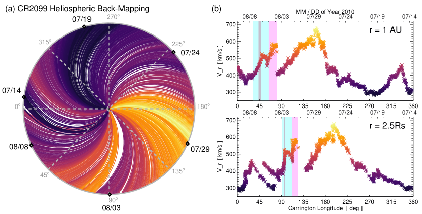
Figure 14 illustrates the back-mapping procedure for CR2099 which starts at 2010-07-13 09:38UT and goes through 2010-08-09 14:48UT. Figure 14(a) plots the Parker spiral streamlines, color-coded by radial velocity. Figure 14(b) plots the bulk proton radial velocity in 1-hour averages measured by ACE at 1 AU in Carrington longitude (here time runs from right-to-left, as indicated with the top -axis labels). The vertical bars identify three in–situ intervals that are highlighted in Figure 15 and are discussed in detail below: magenta indicates an ICME interval, cyan indicates the estimated time of arrival of the jet material, and the red/orange region within the cyan interval has a distinct elemental composition. The estimated arrival time of the 2010-08-02 coronal jet material is taken to be between DOY 217.0 (August 05) to DOY 219.5 (August 07 12:00UT) corresponding to the range of Carrington longitudes 31.6–64.3∘ at 1 AU. This range maps back to Carrington longitudes 91.3–111.7∘ at , or equivalently, comfortably within the 10∘ range of the central meridian (Carrington longitude ) on August 02, which is indeed the location of the spot (see Figure 3).
In–situ measurements of the solar wind and our jet interval of interest were investigated using MAG (Smith et al., 1998), Solar Wind Electron Proton Alpha Monitor (SWEPAM) (McComas et al., 1998), and Solar Wind Ion Composition Spectrometer (SWICS) (Gloeckler et al., 1998) instruments on the Advanced Composition Explorer (ACE; Stone et al., 1998), along with the 3DP instrument (Lin et al., 1995) on the Wind spacecraft showing the pitch angle distribution of electron flux. Figure 15 is a multipanel plot showing solar wind properties at the ACE instruments for panels 15(a)–(j) and at Wind for panel 15(k).
The purple box across the data shows an ICME interval with boundaries taken from Richardson and Cane (2010). The ICME-driven shock arrives on August 3 at 17:00UT followed by a large sheath region and what appears to be two coherent magnetic flux rope ejecta (e.g., see Harrison et al., 2012; Möstl et al., 2012). The ICME interval exhibits distinct in–situ ionic and elemental composition signatures that have been interpreted as filament material (Sharma and Srivastava, 2012), which may be expected from previous analyses (e.g. Lepri and Zurbuchen, 2010; Lepri and Rivera, 2021). This ICME period has been linked to a series of three sequential CME eruptions of large, quiescent filaments on August 1st at 06:30UT, 16:30UT, and 21:00UT (e.g. Schrijver and Title, 2011; Török et al., 2011; Temmer et al., 2012). The filament channel source region of the third eruption is approximately 30∘ west and 15–20∘ north of AR 11092 and its quiescent filament erupts 20 hr earlier than our jet event on August 2nd.
The blue shaded region is the predicted arrival period of the jet using the ballistic back-mapping from Figure 14. The blue shaded region is characterized by a period of steady km s-1 wind followed by monotonically decreasing speed towards the second half as shown in panel 15(g). The proton temperature remains between K, and the density cm-3, both typical properties of fast solar wind.
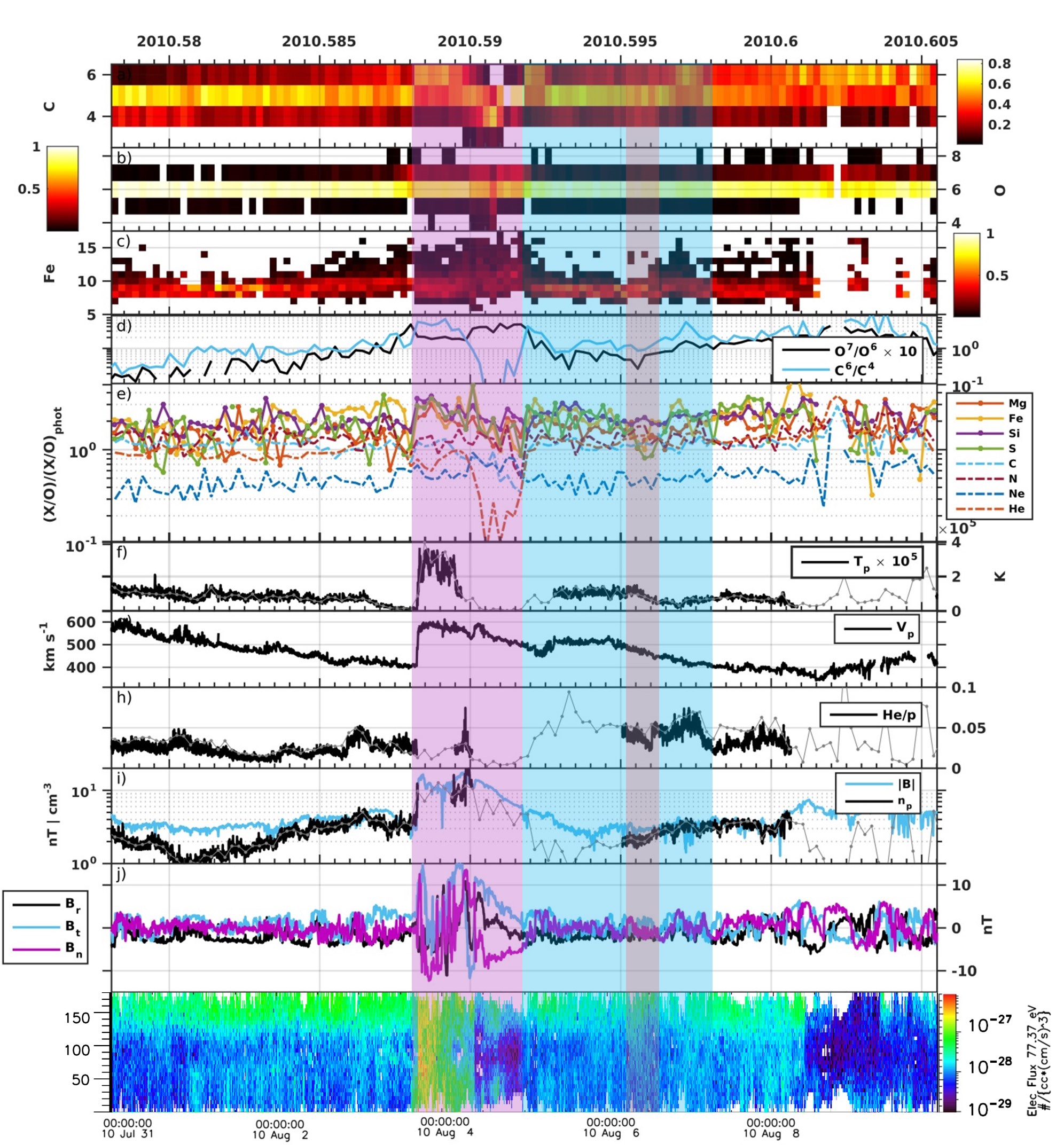
The relative ionization fractions of C , O , and Fe , respectively, shown in panels 15(a)–(c) are observed to shift to higher ionized states, with elevated C6+ and O7+ along with the appearance of higher ionized Fe charge states, Fe>12+, towards the second half of the blue region. This is also seen in panel 15(d) showing elevated values of O7+/O6+ and C6+/C4+ indicating higher coronal temperature or higher coronal densities. Panel 15(e) shows the FIP bias as X/O/X/Ophot for each element, X, listed. Within the blue region we see a gradual decrease in the abundance of low FIP elements Mg , Fe , Si and high FIP S relative to O that initially range between begin to dip below 2 within the red box. Other ratios, Ne /O , N /O , C /O and He /O hardly change. The fact that S /O is high in the blue region suggests an origin in strong open magnetic fields, with its decrease in the red region, more pronounced than the decrease in any other element, implies either a weaker magnetic field open region, or a closed loop as the origin for this plasma. Other abundance ratios are not so conclusive. Ne /O strongly favours a closed loop origin, C /O and N /O favour open field, while He /O here measured above 1 is at variance with expectations from He /H in panel 15(h), typically about 0.5 for an absolute abundance ratio of about 0.04. Although not purely photospheric, this transition to near photospheric abundances in Mg /O , Fe /O , Si /O , and S /O along with a reduction in the ionization stage of charge states, may also be an indication that its source lies deeper in the chromosphere. These properties may also suggest that the ejection site was already at open field lines with plasma flowing out with coronal composition as we inferred with our EUV and MHD analysis while the shift to lower FIP values within the jet structure may indicate the plasma ejected also contained some mixture of coronal and chromospheric composition.
Moreover, prior to the red region within the blue box, the temperature and velocity increase slightly then remain steady before reaching the red box as shown in panel 15(f)–(g). This period also shows enriched He/p, values as seen in ICMEs (Hirshberg et al., 1972; Borrini et al., 1983). The red box marks a transition to cooler proton temperature and monotonically decreasing velocity values indicating a rapid expansion in the plasma. Furthermore, the period within the blue box is characterized by low magnetic field magnitude, as shown in panel 15(i), where B gradually decreases and remains below 5 nT while the magnetic field components in panel 15(j) show small fluctuations in the BN and BT and a steady BR component. During this period in blue, the IMF points back towards the Sun, where B, B, and B. This can also be observed with the electron pitch angle distributions in panel 15(k) which observe an uninterrupted concentrated beam of electrons directed towards the Sun, anti parallel (135–180∘) to the interplanetary magnetic field (IMF), that are likely rooted at the Sun.
5 Discussion and Conclusions
In this work we have combined data and modelling work in order to reconstruct the solar and heliospheric magnetic and plasma properties for the days around the appearance of a coronal jet. The goal was to show that it is possible to reconcile data and modeling results, and that they should be used together to provide all the elements to reconstruct the history of this ejection from its solar source to its possible travel into the interplanetary medium. This event was taken as test case in preparation of the Solar Orbiter data exploitation. The main results are summarized and discussed in the following.
The large scale coronal magnetic field distribution for the day of the jet was obtained applying different methods and initial conditions (Sections 4.1). The results are consistent in finding open flux nearby the spot at the jet location that is, a channel through which active region plasma can flow and reach the interplanetary medium.
A more detailed analysis in the spot and nearby areas, which takes account of the local temporal variation of the magnetic field, also indicates the presence of a pseudostreamer-like closed-flux system west of the spot. This configuration can easily produce reconnection followed by plasma ejection in the adjacent created open field lines (Sections 4.2 and 4.3). The footpoints of the open area adjacent to the spot are present before, during and after the ejection, even though with some morphological change. These together with the signatures of reconnection (HXR emission) and flux emergence found by Mulay et al. (2016), are consistent with reconnection (possibly interchange type) and re-organization of the magnetic field.
The additional information provided by the EUV coronal observations is the presence of upflows in these open regions before, during and after the jet, as well as small scale dynamics activity in the jet channel. This reinforces the picture where plasma from the spot flows out in the open corona. As discussed in Section 4.5 and shown in Figure 13 our MHD model reproduces consistently the plasma outflow from EUV observations and the magnetic field environment.
Our magnetic field analysis highlights one of the known critical key points affecting the quality of the results, that is the important role of the magnetic map built from observations and used to extrapolate the initial field. We have seen in Section 3.1 that low spatial resolution and/or insufficient updates of the map can negatively affect the extrapolation. Having a second magnetometer, such as the Solar Orbiter/PHI, observing at different angles than the Earth view, will allow to have a much frequent update of such maps, including information like the backside face of the Sun. This is a major improvement which will reduce uncertainties on the magnetic field temporal variation. Additionally, the reduced solar distance together with the high spatial resolution of the PHI instrument, will provide high quality data for local magnetic field analysis.
Solar Orbiter also will leave the ecliptic plane and reach about 30∘ in latitude, allowing for the first time a view of the solar poles. This will be a major input for the study of the solar magnetic field with the consequent improvement of the global magnetic field modelling.
Solar Orbiter carries the UV spectrometer SPICE which, for the first time, will provide data (even though not on a continuous observation basis) to perform spectro-stereoscopy (e.g. Podladchikova, 2021) with other Earth view observatories such as IRIS and Hinode/EIS. One of the major potential advantages of these multi-point of view measurements is the reconstruction of the 3D vector velocity through Doppler measurements. These measures will allow a better identification and characterization of the outflow regions even in magnetically complex areas as active regions, and they will permit a more direct comparison with the magnetic field extrapolation. Furthermore, having the real amplitude of the plasma outflow will provide stronger constraints to the wind and FIP bias models, as well as back mapping diagnostics and in–situ data comparison. Unfortunately the remote sensing instruments on board Solar Orbiter cannot observe on daily basis, as done by the other existing EUV-UV spectrometers or imagers positioned at Earth distance, so that these unique multi-point of view configurations remain occasional.
In this work we use the plasma FIP bias as a tool for the connectivity between the heliosphere and its source regions on the Sun. Using two independent methods applied to the EUV data we found the outflow open areas at the side of the spot to be the source of coronal FIP biased plasma (Sections 4.4.1 and 4.4.2). Using the results from the coronal MHD model we simulated the strength of the FIP fractionation in the magnetically open and closed selected areas (Sections 4.5 and 4.6). In some cases the results show a clear difference between these two regions, with the closed areas affected by a more important fractionation, consistently with the results from the EUV data. However, one of the closed areas (CO1) shows a less pronounced FIP bias. This is a case where further investigation would be needed. In fact, such result may be consistent with a low FIP bias coming from closed regions which have been opened up as consequence of local magnetic reconnection. Fractionation in both open and closed field regions increases with increasing magnetic field strength, but in different ways, and also depends on the degree to which Alfvén waves dominate over compressive fluctuations (the Alfvénicity). In closed field it is also sensitive to how close the Alfvén waves are to resonance with the loop (i.e. when the wave travel time from one footpoint to the other is to an integral number of wave half-periods). Such constraints provide significant distinct FIP fractionation imprints depending on these parameters, providing a potential tool for selecting the most appropriate source regions of the plasma measured in–situ. As a consequence we emphasize the importance of having, additionally to a high quality magnetic field instruments, in–situ measures of the Alfveńicity as close as possible to the Sun, and in conjunction with solar FIP bias at candidate solar locations. This exactly what Solar Orbiter provides. These in–situ measures will be less affected by modification resulting from the interaction with the local magnetic field and plasma as the wind travels through the heliosphere.
From in–situ observations within the period where the jet is predicted through the backmapping method, measurements show some changes in both the chemical composition and ionization level of charge states along with temperature and velocity that may suggest some part of the jet may have been observed. In particular, the closed field with resonant Alfvén waves does not fractionate S, but open field can, depending on magnetic field strength. The observations in Table 4 and models in Table 5 do not see or predict significant fractionation in S, and this matches almost exclusively with the latter part of the putative “jet” in Figure 15 denoted by the red shaded column beginning approximately at 2010 August 6, 05:00:00, which illustrates the utility of abundances in identifying solar wind sources regions. However, the in–situ measurements show no other relevant signatures of the jet structure.
We do not think the jet signature is intertwined or overwhelmed by the ICME passage. The beginning of the ICME has a moderately strong FIP effect, but not so large as to be remarkable in remote sensing observations. The strong depletion of He towards the end of the ICME however is remarkable. It has not been possible to model depletion of He down to He/O 1% with the ponderomotive force model. This degree of depletion presumably indicates gravitational settling in a closed loop prior to eruption (e.g Laming et al., 2019).
Furthermore, jet may have evolved and expanded such that it is indistinguishable from the surrounding solar wind. Another possibility could be that the instruments at 1AU do not measure the main jet structure missing the majority of the ejected jet material. This demonstrates the need for additional in–situ measurements made closer to the Sun, such as those that are made by Solar Orbiter and Parker Solar Probe where smaller structures, the jets in this case, are easier to distinguish from solar wind and can be more effectively traced back to the Sun. This understanding of the spatial and temporal evolution of magnetic and plasma structures as they travel through the heliosphere is a major challenge, and multi-measurement observations at different distances is the ideal thing to have to resolve this aspect. The monitoring of the heliosphere in the neighbour of the Earth remains, however, fundamental in the frame of the Space Weather forecasting, as well as to understand the physical processes dominating the diluted plasma and magnetic field of the heliopshere.
Another advantage of additional in-situ measurements below 1 AU, is that measurements of heavy ions, such as those from the Heavy Ion Sensor (HIS) (Owen et al., 2020) on Solar Orbiter, can be taken at higher resolution compared to 1AU that will allow for more detailed characterization of jet substructure to study the plasma origin, release, and evolution from the Sun.
In conclusion, with this work we have shown that collaborative data and modelling efforts are essential to build a comprehensive picture which allows to trace and follow the plasma travelling through the heliosphere. This is needed to identify the heliosphere and solar wind sources regions. We have also discussed the difficulties of our work which was limited, beside others, by the available UV and in–situ data. With the Solar Orbiter entering the nominal mission phase in 2022 we expect most of these limitations to be solved.
Declarations
-
Funding: This work was supported by the International Space Science Institute through its International Team program.
-
Availability of data and materials: The Hinode/EIS data are freely available through the European Hinode Data Cente: http://sdc.uio.no/sdc/.
STEREO and SDO/AIA data are available through the MEDOC datacenter: https://idoc-medoc.ias.u-psud.fr/sitools/client-user/index.html?project=Medoc-Solar-Portal.
GONG synoptic maps: ftp://gong2.nso.edu/oQR/zqs/201008/mrzqs100802/mrzqs100802t1154c2099_034.fits.gz.
SDO/HMI radial field synoptic map: http://jsoc.stanford.edu/data/hmi/synoptic/hmi.Synoptic_Mr_small.2099.fits.
-
Code availability:
The CHIANTI and ChiantiPy atomic database and software for the EUV diagnostic analysis666http://www.chiantidatabase.org/ are freely available through SolarSoft: https://www.lmsal.com/solarsoft/.
The PFSS extrapolations are based on an IDL implementation of the current-free case of the formula presented in Zhao and Hoeksema (1993). Our results are comparable to those obtained with the PFSS package provided in SolarSoft: https://www.lmsal.com/~derosa/pfsspack/.
The Adaptively Refined MHD Solver (ARMS; DeVore and Antiochos, 2008) is a proprietary research code designed for massively parallel high-performance computing clusters such as the NASA Center for Climate Simulation. For queries about the ARMS simulation data herein or the IDL post-processing analysis routines, please contact blynch@berkeley.edu. For queries about ARMS, including obtaining the source code, please contact c.richard.devore@nasa.gov.
FIPLCR finds the optimal linear combination of EUV spectral lines for calculating the FIP bias using the LCR method: https://git.ias.u-psud.fr/nzambran/fiplcr
Acknowledgements.
This collaborative work was made with the support of the International Space Science Institute through its International Team program (Team 418). S.P. acknowledges the funding by CNES through the MEDOC data and operations center. S.P. is grateful to Dr. Hans-Peter Doerr for the discussion on images co-registration. B.J.L. was supported in part by NASA grants 80NSSC18K0645, 80NSSC18K1553, and 80NSSC20K1448. J.M.L. was supported by the NASA Heliophysics Guest Investigator (80HQTR19T0029) and Supporting Research Programs (80HQTR20T0076), and by Basic Research Funds of the Office of Naval Research. I.C. acknowledges DFG-grant WI 3211/5-1. G.D.Z. acknowledges support from STFC (UK) via the consolidated grants to the atomic astrophysics group at DAMTP, University of Cambridge (ST/P000665/1. and ST/T000481/1). T.W. acknowledges financial support by DLR-grants 50 OC 1701 and 50 OC 2101 and DFG-grant WI 3211/5-1. Y.J.R. acknowledges support from the Rackham Merit Fellowship at the University of Michigan, the Newkirk Fellowship at the High Altitude Observatory, and Future Faculty Leaders Fellowship at the Center for Astrophysics. S.T.L. acknowledges support from NASA grants: NNX16AP03H, NNX16AH01G, and 80NSSC20K1063; NSF Grants: 1460170 and AGS 1358268; and DOD Grant: N00173-14-1-G904. R.F.W-S. acknowledges DLR grant 50OT1702 and DFG grant WI 2139/11-1. G.P. has received funding from the European Research Council (ERC) under the European Union’s Horizon 2020 research and innovation program (grant agreement No. 724326). CHIANTI is a collaborative project involving George Ma-son University, the University of Michigan, the NASA Goddard Space Flight Centre (USA) and the University of Cambridge (UK). Hinode is a Japanese mission developed and launched by ISAS/JAXA, with NAOJ as domestic partner and NASA and UKSA as international partners. It is operated by these agencies in co-operation with ESA and NSC (Norway). "Courtesy of NASA/SDO and the AIA, EVE, and HMI science teams." The EUVI images are supplied courtesy of the STEREO Sun Earth Connection Coronal and Heliospheric Investigation (SECCHI) team.References
- Abbo et al. (2016) Abbo L, Ofman L, Antiochos SK, Hansteen VH, Harra L, Ko YK, Lapenta G, Li B, Riley P, Strachan L, von Steiger R, Wang YM (2016) Slow Solar Wind: Observations and Modeling. Space Sci. Rev., 201(1-4):55–108, DOI: 10.1007/s11214-016-0264-1
- Altschuler and Newkirk (1969) Altschuler MD, Newkirk G (1969) Magnetic Fields and the Structure of the Solar Corona. I: Methods of Calculating Coronal Fields. Solar Phys., 9:131–149, DOI: 10.1007/BF00145734
- Antiochos et al. (2011) Antiochos SK, Mikić Z, Titov VS, Lionello R, Linker JA (2011) A Model for the Sources of the Slow Solar Wind. Astrophys. J., 731:112, DOI: 10.1088/0004-637X/731/2/112, 1102.3704
- Arge et al. (2004) Arge CN, Luhmann JG, Odstrcil D, Schrijver CJ, Li Y (2004) Stream structure and coronal sources of the solar wind during the May 12th, 1997 CME. Journal of Atmospheric and Solar-Terrestrial Physics, 66(15-16):1295–1309, DOI: 10.1016/j.jastp.2004.03.018
- Asplund et al. (2009) Asplund M, Grevesse N, Sauval AJ, Scott P (2009) The Chemical Composition of the Sun. Annu. Rev. Astron. Astrophys., 47:481–522, DOI: 10.1146/annurev.astro.46.060407.145222, 0909.0948
- Badman et al. (2020) Badman ST, Bale SD, Martínez Oliveros JC, Panasenco O, Velli M, Stansby D, Buitrago-Casas JC, Réville V, Bonnell JW, Case AW, Dudok de Wit T, Goetz K, Harvey PR, Kasper JC, Korreck KE, Larson DE, Livi R, MacDowall RJ, Malaspina DM, Pulupa M, Stevens ML, Whittlesey PL (2020) Magnetic Connectivity of the Ecliptic Plane within 0.5 au: Potential Field Source Surface Modeling of the First Parker Solar Probe Encounter. Astrophys. J. Suppl., 246(2):23, DOI: 10.3847/1538-4365/ab4da7
- Baker et al. (2018) Baker D, Brooks DH, van Driel-Gesztelyi L, James AW, Démoulin P, Long DM, Warren HP, Williams DR (2018) Coronal Elemental Abundances in Solar Emerging Flux Regions. Astrophys. J., 856:71, DOI: 10.3847/1538-4357/aaadb0, 1801.08424
- Bemporad et al. (2003) Bemporad A, Poletto G, Suess ST, Ko YK, Parenti S, Riley P, Romoli M, Zurbuchen TZ (2003) Temporal Evolution of a Streamer Complex: Coronal and in Situ Plasma Parameters. Astrophys. J., 593(2):1146–1163, DOI: 10.1086/376605
- Bochsler (2007) Bochsler P (2007) Minor ions in the solar wind. Astron Astrophys Rev, 14:1–40, DOI: 10.1007/s00159-006-0002-x
- Borrini et al. (1983) Borrini G, Gosling JT, Bame SJ, Feldman WD (1983) Helium Abundance Variations in the Solar Wind. Solar Phys., 83(2):367–378, DOI: 10.1007/BF00148286
- Bürgi and Geiss (1986) Bürgi A, Geiss J (1986) Helium and minor ions in the corona and solar wind - Dynamics and charge states. Solar Phys., 103:347–383, DOI: 10.1007/BF00147835
- Bučík (2020) Bučík R (2020) 3He-Rich Solar Energetic Particles: Solar Sources. Space Sci. Rev., 216(2):24, DOI: 10.1007/s11214-020-00650-5, 2002.09442
- Cheung and DeRosa (2012) Cheung MCM, DeRosa ML (2012) A Method for Data-driven Simulations of Evolving Solar Active Regions. Astrophys. J., 757(2):147, DOI: 10.1088/0004-637X/757/2/147, 1208.2954
- Corti et al. (2007) Corti G, Poletto G, Suess ST, Moore RL, Sterling AC (2007) Cool-Plasma Jets that Escape into the Outer Corona. Astrophys. J., 659(2):1702–1712, DOI: 10.1086/512233
- Cranmer (2012) Cranmer SR (2012) Self-Consistent Models of the Solar Wind. Space Sci. Rev., 172(1-4):145–156, DOI: 10.1007/s11214-010-9674-7, 1007.0954
- Cranmer et al. (1999) Cranmer SR, Kohl JL, Noci G, Antonucci E, Tondello G, Huber MCE, Strachan L, Panasyuk AV, Gardner LD, Romoli M, Fineschi S, Dobrzycka D, Raymond JC, Nicolosi P, Siegmund OHW, Spadaro S, Benna C, Ciaravella A, Giordano S, Habbal SR (1999) An empirical model of a polar coronal hole at solar minimum. Astrophys J, 511:481–501, DOI: 0.1086/306675
- Cranmer et al. (2008) Cranmer SR, Panasyuk AV, Kohl JL (2008) Improved constraints on the preferential heating and acceleration of oxygen ions in the extended solar corona. Astrophys J, 678:1480–1497, DOI: 10.1086/586890, arXiv:0802.0144
- Culhane et al. (2007) Culhane JL, Harra LK, James AM, Al-Janabi K, Bradley LJ, Chaudry RA, Rees K, Tandy JA, Thomas P, Whillock MCR, Winter B, Doschek GA, Korendyke CM, Brown CM, Myers S, Mariska J, Seely J, Lang J, Kent BJ, Shaughnessy BM, Young PR, Simnett GM, Castelli CM, Mahmoud S, Mapson-Menard H, Probyn BJ, Thomas RJ, Davila J, Dere K, Windt D, Shea J, Hagood R, Moye R, Hara H, Watanabe T, Matsuzaki K, Kosugi T, Hansteen V, Wikstol Ø (2007) The EUV Imaging Spectrometer for Hinode. Solar Phys., 243:19–61
- Dahlburg et al. (2016) Dahlburg RB, Laming JM, Taylor BD, Obenschain K (2016) Ponderomotive Acceleration in Coronal Loops. Astrophys. J., 831(2):160, DOI: 10.3847/0004-637X/831/2/160, 1608.04372
- Dahlin et al. (2019) Dahlin JT, Antiochos SK, DeVore CR (2019) A Model for Energy Buildup and Eruption Onset in Coronal Mass Ejections. Astrophys. J., 879(2):96, DOI: 10.3847/1538-4357/ab262a, 1905.13218
- de Pablos et al. (2021) de Pablos D, Long DM, Owen CJ, Valori G, Nicolaou G, Harra LK (2021) Matching Temporal Signatures of Solar Features to Their Corresponding Solar-Wind Outflows. Solar Phys., 296(4):68, DOI: 10.1007/s11207-021-01813-5, 2103.09077
- Del Zanna (1999) Del Zanna G (1999) Extreme ultraviolet spectroscopy of the solar corona. PhD thesis, University of Central Lancashire, UK, URL http://www.damtp.cam.ac.uk/user/astro/gd232/research/thesis/gdz_phd_thesis.pdf
- Del Zanna (2013) Del Zanna G (2013) A revised radiometric calibration for the Hinode/EIS instrument. Astron. Astrophys., 555:A47, DOI: 10.1051/0004-6361/201220810, 1211.6771
- Del Zanna (2019) Del Zanna G (2019) The EUV spectrum of the Sun: Quiet- and active-Sun irradiances and chemical composition. Astron. Astrophys., 624:A36, DOI: 10.1051/0004-6361/201834842, 1901.08841
- Del Zanna and Mason (2018) Del Zanna G, Mason HE (2018) Solar UV and X-ray spectral diagnostics. Living Rev. Sol. Phys., 15:5, DOI: 10.1007/s41116-018-0015-3
- Del Zanna et al. (2015) Del Zanna G, Dere KP, Young PR, Landi E, Mason HE (2015) CHIANTI - An atomic database for emission lines. Version 8. Astron. Astrophys., 582:A56, DOI: 10.1051/0004-6361/201526827, 1508.07631
- Dere et al. (1997) Dere KP, Landi E, Mason HE, Monsignori Fossi BC, Young PR (1997) Chianti - an atomic database for emission lines. Astron. Astrophys. Suppl., 125:149–173
- Dere et al. (2019) Dere KP, Del Zanna G, Young PR, Landi E, Sutherland RS (2019) dere19—An Atomic Database for Emission Lines. XV. Version 9, Improvements for the X-Ray Satellite Lines. Astrophys. J. Suppl., 241:22, DOI: 10.3847/1538-4365/ab05cf, 1902.05019
- DeRosa and Barnes (2018) DeRosa ML, Barnes G (2018) Does Nearby Open Flux Affect the Eruptivity of Solar Active Regions? Astrophys. J., 861(2):131, DOI: 10.3847/1538-4357/aac77a, 1802.01199
- DeVore (1991) DeVore CR (1991) Flux-corrected transport techniques for multidimensional compressible magnetohydrodynamics. J. Comp. Phys., 92:142–160, DOI: 10.1016/0021-9991(91)90295-V
- DeVore and Antiochos (2008) DeVore CR, Antiochos SK (2008) Homologous Confined Filament Eruptions via Magnetic Breakout. Astrophys. J., 680:740–756, DOI: 10.1086/588011
- Domingo et al. (1995) Domingo V, Fleck B, Poland AI (1995) The SOHO Mission: an Overview. Solar Phys., 162(1-2):1–37, DOI: 10.1007/BF00733425
- Drake et al. (1997) Drake JJ, Laming JM, Widing KG (1997) Stellar coronal abundances. v. evidence for the first ionization potential effect in alpha centauri. Astrophys J, 478:403–416, DOI: 10.1086/303755
- Dufresne and Del Zanna (2019) Dufresne RP, Del Zanna G (2019) Modelling ion populations in astrophysical plasmas: carbon in the solar transition region. Astron. Astrophys., 626:A123, DOI: 10.1051/0004-6361/201935133, 1901.08992
- Dufresne et al. (2020) Dufresne RP, Del Zanna G, Badnell NR (2020) Effects of density on the oxygen ionization equilibrium in collisional plasmas. Mon. Not. Roy. Astron. Soc., 497(2):1443–1456, DOI: 10.1093/mnras/staa2005, 2007.00465
- Edmondson and Lynch (2017) Edmondson JK, Lynch BJ (2017) Formation and Reconnection of Three-dimensional Current Sheets with a Guide Field in the Solar Corona. Astrophys. J., 849:28, DOI: 10.3847/1538-4357/aa83ba
- Edmondson et al. (2010) Edmondson JK, Antiochos SK, DeVore CR, Lynch BJ, Zurbuchen TH (2010) Interchange Reconnection and Coronal Hole Dynamics. Astrophys. J., 714:517–531, DOI: 10.1088/0004-637X/714/1/517
- Feldman (1992) Feldman U (1992) Elemental abundances in the upper solar atmosphere. Phys. Scripta, 46:202–220
- Fisk and Schwadron (2001) Fisk LA, Schwadron NA (2001) The Behavior of the Open Magnetic Field of the Sun. Astrophys. J., 560(1):425–438, DOI: 10.1086/322503
- Frazin et al. (1999) Frazin RA, Ciaravella A, Dennis E, Fineschi S, Gardner LD, Michels DJ, O’Neal R, Raymond JC, Wu CR, Kohl JL, Modigliani A, Noci G (1999) Uvcs/soho ion kinetics in coronal streamers. Space Science Rev, 87:189–192, DOI: 10.1023/A:1005184014654
- Geiss et al. (1995) Geiss J, Gloeckler G, von Steiger R (1995) Origin of the Solar Wind From Composition Data. Space Sci. Rev., 72(1-2):49–60, DOI: 10.1007/BF00768753
- Gibson et al. (2011) Gibson SE, de Toma G, Emery B, Riley P, Zhao L, Elsworth Y, Leamon RJ, Lei J, McIntosh S, Mewaldt RA, Thompson BJ, Webb D (2011) The Whole Heliosphere Interval in the Context of a Long and Structured Solar Minimum: An Overview from Sun to Earth. Solar Phys., 274:5–27, DOI: 10.1007/s11207-011-9921-4
- Giunta et al. (2015) Giunta AS, Fludra A, Lanzafame AC, O’Mullane MG, Summers HP, Curdt W (2015) On Extreme-ultraviolet Helium Line Intensity Enhancement Factors on the Sun. Astrophys. J., 803(2):66, DOI: 10.1088/0004-637X/803/2/66
- Gloeckler et al. (1998) Gloeckler G, Cain J, Ipavich FM, Tums EO, Bedini P, Fisk LA, Zurbuchen TH, Bochsler P, Fischer J, Wimmer-Schweingruber RF, Geiss J, Kallenbach R (1998) Investigation of the composition of solar and interstellar matter using solar wind and pickup ion measurements with SWICS and SWIMS on the ACE spacecraft. Space Sci. Rev., 86:497–539, DOI: 10.1023/A:1005036131689
- Gruesbeck et al. (2011) Gruesbeck JR, Lepri ST, Zurbuchen TH, Antiochos SK (2011) Constraints on Coronal Mass Ejection Evolution from in Situ Observations of Ionic Charge States. Astrophys. J., 730:103, DOI: 10.1088/0004-637X/730/2/103
- Hansteen and Velli (2012) Hansteen VH, Velli M (2012) Solar Wind Models from the Chromosphere to 1 AU. Space Sci. Rev., 172(1-4):89–121, DOI: 10.1007/s11214-012-9887-z
- Harra et al. (2021) Harra L, Brooks DH, Bale SD, Mandrini CH, Barczynski K, Sharma R, Badman ST, Vargas Domínguez S, Pulupa M (2021) The active region source of a type III radio storm observed by Parker Solar Probe during encounter 2. Astron. Astrophys., 650:A7, DOI: 10.1051/0004-6361/202039514, 2102.04964
- Harrison et al. (2012) Harrison RA, Davies JA, Möstl C, Liu Y, Temmer M, Bisi MM, Eastwood JP, de Koning CA, Nitta N, Rollett T, Farrugia CJ, Forsyth RJ, Jackson BV, Jensen EA, Kilpua EKJ, Odstrcil D, Webb DF (2012) An Analysis of the Origin and Propagation of the Multiple Coronal Mass Ejections of 2010 August 1. Astrophys. J., 750(1):45, DOI: 10.1088/0004-637X/750/1/45
- Heber et al. (2021) Heber VS, Burnett DS, McKeegan KD, Steele RCJ, Jurewicz AJG, Rieck KD, Guan Y, Wieler R, Burnett DS (2021) Elemental abundances of major elements in the solar wind as measured in genesis targets and implications on solar wind fractionation. Astrophys J, 907:15, DOI: 10.3847/1538-4357/abc94a
- Higginson and Lynch (2018) Higginson AK, Lynch BJ (2018) Structured Slow Solar Wind Variability: Streamer-blob Flux Ropes and Torsional Alfvén Waves. Astrophys. J., 859:6, DOI: 10.3847/1538-4357/aabc08
- Higginson et al. (2017a) Higginson AK, Antiochos SK, DeVore CR, Wyper PF, Zurbuchen TH (2017a) Dynamics of Coronal Hole Boundaries. Astrophys. J., 837:113, DOI: 10.3847/1538-4357/837/2/113, 1611.04968
- Higginson et al. (2017b) Higginson AK, Antiochos SK, DeVore CR, Wyper PF, Zurbuchen TH (2017b) The Formation of Heliospheric Arcs of Slow Solar Wind. Astrophys. J. Lett., 840(1):L10, DOI: 10.3847/2041-8213/aa6d72, 1701.08797
- Hill (2018) Hill F (2018) The Global Oscillation Network Group Facility—An Example of Research to Operations in Space Weather. Space Weather, 16(10):1488–1497, DOI: 10.1029/2018SW002001
- Hirshberg et al. (1972) Hirshberg J, Bame SJ, Robbins DE (1972) Solar flares and solar wind helium enrichments: July 1965 July 1967. Solar Phys., 23(2):467–486, DOI: 10.1007/BF00148109
- Hoeksema (1991) Hoeksema JT (1991) Large-scale solar and heliospheric magnetic fields. Adv. Space Res., 11(1):15–24
- Hoeksema et al. (1983) Hoeksema JT, Wilcox JM, Scherrer PH (1983) The structure of the heliospheric current sheet: 1978-1982. J. Geophys. Res., 88(A12):9910–9918, DOI: 10.1029/JA088iA12p09910
- Hoeksema et al. (2020) Hoeksema JT, Abbett WP, Bercik DJ, Cheung MCM, DeRosa ML, Fisher GH, Hayashi K, Kazachenko MD, Liu Y, Lumme E, Lynch BJ, Sun X, Welsch BT (2020) The Coronal Global Evolutionary Model: Using HMI Vector Magnetogram and Doppler Data to Determine Coronal Magnetic Field Evolution. Astrophys. J. Suppl., 250(2):28, DOI: 10.3847/1538-4365/abb3fb, 2006.14579
- Hundhausen (1972) Hundhausen AJ (1972) Coronal Expansion and Solar Wind. Springer-Verlag, Berlin
- Hundhausen et al. (1968) Hundhausen AJ, Gilbert HE, Bame SJ (1968) The State of Ionization of Oxygen in the Solar Wind. Astrophys. J. Lett., 152:L3, DOI: 10.1086/180165
- Innes et al. (2011) Innes DE, Cameron RH, Solanki SK (2011) EUV jets, type III radio bursts and sunspot waves investigated using SDO/AIA observations. Astron. Astrophys., 531:L13, DOI: 10.1051/0004-6361/201117255, 1106.3417
- Karpen et al. (2012) Karpen JT, Antiochos SK, DeVore CR (2012) The Mechanisms for the Onset and Explosive Eruption of Coronal Mass Ejections and Eruptive Flares. Astrophys. J., 760:81, DOI: 10.1088/0004-637X/760/1/81
- Karpen et al. (2017) Karpen JT, DeVore CR, Antiochos SK, Pariat E (2017) Reconnection-Driven Coronal-Hole Jets with Gravity and Solar Wind. Astrophys. J., 834:62, DOI: 10.3847/1538-4357/834/1/62, 1606.09201
- Ko et al. (1997) Ko YK, Fisk LA, Geiss J, Gloeckler G, Guhathakurta M (1997) An Empirical Study of the Electron Temperature and Heavy Ion Velocities in the South Polar Coronal Hole. Solar Phys., 171:345–361
- Ko et al. (2016) Ko YK, Young PR, Muglach K, Warren HP, Ugarte-Urra I (2016) Correlation of Coronal Plasma Properties and Solar Magnetic Field in a Decaying Active Region. Astrophys. J., 826:126, DOI: 10.3847/0004-637X/826/2/126
- Ko et al. (2018) Ko YK, Roberts DA, Lepri ST (2018) Boundary of the slow solar wind. Astrophys J, 864:139, DOI: 10.3847/1538-4357/aad69e
- Kohl et al. (1997) Kohl JL, Noci G, Antonucci E, Huber MCE, Gardner LD, Nicolosi P, Strachan L, Fineschi S, Raymond JC, Romoli M, Spadaro D, Panasyuk AV, Siegmund OHW, Benna C, Ciaravella A, Cranmer SR, Giordano S, Karovska M, Martin R (1997) First results from the soho ultraviolet coronagraph spectrometer. Solar Phys, 175:613–644, DOI: 10.1023/A:1004903206467
- Kohl et al. (1998) Kohl JL, Noci G, Antonucci E, Tondello G, Huber SR M C Eand Cranmer, Strachan L, Panasyuk AV, Gardner LD, Romoli M, Fineschi S, Dobrzycka D, Raymond JC, Nicolosi P, Siegmund OH, Spadaro D, Benna C, Ciaravella A, Giordano S, Habbal SR (1998) Uvcs/soho empirical determinations of anisotropic velocity distributions in the solar corona. Astrophys J Lett, 501:L127–L131, DOI: 10.1086/311434
- Kohl et al. (2006) Kohl JL, Noci G, Cranmer SR, Raymond JC (2006) Ultraviolet spectroscopy of the extended solar corona. Astron Astrophys Rev, 13:31–157, DOI: 10.1086/510710
- Krucker et al. (2020) Krucker S, Hurford GJ, Grimm O, Kögl S, Gröbelbauer HP, Etesi L, Casadei D, Csillaghy A, Benz AO, Arnold NG, Molendini F, Orleanski P, Schori D, Xiao H, Kuhar M, Hochmuth N, Felix S, Schramka F, Marcin S, Kobler S, Iseli L, Dreier M, Wiehl HJ, Kleint L, Battaglia M, Lastufka E, Sathiapal H, Lapadula K, Bednarzik M, Birrer G, Stutz S, Wild C, Marone F, Skup KR, Cichocki A, Ber K, Rutkowski K, Bujwan W, Juchnikowski G, Winkler M, Darmetko M, Michalska M, Seweryn K, Białek A, Osica P, Sylwester J, Kowalinski M, Ścisłowski D, Siarkowski M, Stęślicki M, Mrozek T, Podgórski P, Meuris A, Limousin O, Gevin O, Le Mer I, Brun S, Strugarek A, Vilmer N, Musset S, Maksimović M, Fárník F, Kozáček Z, Kašparová J, Mann G, Önel H, Warmuth A, Rendtel J, Anderson J, Bauer S, Dionies F, Paschke J, Plüschke D, Woche M, Schuller F, Veronig AM, Dickson ECM, Gallagher PT, Maloney SA, Bloomfield DS, Piana M, Massone AM, Benvenuto F, Massa P, Schwartz RA, Dennis BR, van Beek HF, Rodríguez-Pacheco J, Lin RP (2020) The Spectrometer/Telescope for Imaging X-rays (STIX). Astron. Astrophys., 642:A15, DOI: 10.1051/0004-6361/201937362
- Kruse et al. (2021) Kruse M, Heidrich-Meisner V, Wimmer-Schweingruber RF (2021) Evaluation of a potential field source surface model with elliptical source surfaces via ballistic back mapping of in situ spacecraft data. Astron. Astrophys., 645:A83, DOI: 10.1051/0004-6361/202039120
- Kuroda and Laming (2020) Kuroda N, Laming JM (2020) Magnetic field geometry and composition variation in slow solar winds: The case of sulfur. Astrophys J, 895:36, DOI: 10.3847/1538-4357/ab8870, arXiv:2005.10842
- Laming (2004a) Laming JM (2004a) On collisionless electron-ion temperature equilibration in the fast solar wind. Astrophys J, 604:874–883, DOI: 10.1086/382066, arXiv:astro-ph/0312387
- Laming (2004b) Laming JM (2004b) A unified picture of the first ionization potential and inverse first ionization potential effects. Astrophys J, 614:1063–1072, DOI: 10.1086/423780, arXiv:astro-ph/0405230
- Laming (2009) Laming JM (2009) Non-wkb models of the first ionization potential effect: Implications for solar coronal heating and the coronal helium and neon abundances. Astrophys J, 695:954–969, DOI: 10.1088/0004-637X/695/2/954, arXiv:0901.3350
- Laming (2012) Laming JM (2012) Non-wkb models of the first ionization potential effect: The role of slow mode waves. Astrophys J, 744:115, DOI: 10.1088/0004-637X/744/2/115, arXiv:1110.4357
- Laming (2015) Laming JM (2015) The FIP and Inverse FIP Effects in Solar and Stellar Coronae. Living Rev. Sol. Phys., 12:2, DOI: 10.1007/lrsp-2015-2, 1504.08325
- Laming (2017) Laming JM (2017) The first ionization potential effect from the ponderomotive force: On the polarization and coronal origin of alfvén waves. Astrophys J, 844:153, DOI: 10.3847/1538-4357/aa7cf1, arXiv:1707.05378
- Laming (2021) Laming JM (2021) The fip and inverse fip effects in solar flares. Astrophys J, arXiv:2101.03038
- Laming and Lepri (2007) Laming JM, Lepri ST (2007) Ion Charge States in the Fast Solar Wind: New Data Analysis and Theoretical Refinements. Astrophys. J., 660:1642–1652, DOI: 10.1086/513505, astro-ph/0702131
- Laming and Lepri (2007) Laming JM, Lepri ST (2007) Ion charge states in the fast solar wind: New data analysis and theoretical refinements. Astrophys J, 660:1642–1652, DOI: 10.1086/513505, arXiv:astro-ph/0702131
- Laming et al. (2017) Laming JM, Heber VS, Burnett DS, Guan Y, Hervig R, Huss GR, Jurewicz AJG, Koeman-Shields EC, McKeegan KD, Nittler LR, Reisenfeld DB, Rieck KD, Wang J, Wiens RC, Woolum DS (2017) Determining the elemental and isotopic composition of the pre-solar nebula from genesis data analysis: The case of oxygen. Astrophys J Lett, 851:L12, DOI: 10.3847/2041-8213/aa9bf0, arXiv:1711.07503
- Laming et al. (2019) Laming JM, Vourlidas A, Korendyke C, Chua D, Cranmer SR, Ko YK, Kuroda N, Provornikova E, Raymond JC, Raouafi NE, Strachan L, Tun-Beltran S, Weberg M, Wood BE (2019) Element abundances: A new diagnostic for the solar wind. Astrophys J, 879:124, DOI: 10.3847/1538-4357/ab23f1, arXiv:1905.09319
- Landi et al. (2012) Landi E, Gruesbeck JR, Lepri ST, Zurbuchen TH, Fisk LA (2012) Charge State Evolution in the Solar Wind. II. Plasma Charge State Composition in the Inner Corona and Accelerating Fast Solar Wind. Astrophys. J., 761:48, DOI: 10.1088/0004-637X/761/1/48
- Leamon and McIntosh (2009) Leamon RJ, McIntosh SW (2009) How the Solar Wind Ties to its Photospheric Origins. Astrophys. J. Lett., 697:L28–L32, DOI: 10.1088/0004-637X/697/1/L28, 0904.0614
- Lepri and Rivera (2021) Lepri ST, Rivera YJ (2021) Elemental Abundances of Prominence Material inside ICMEs. Astrophys. J., 912(1):51, DOI: 10.3847/1538-4357/abea9f
- Lepri and Zurbuchen (2010) Lepri ST, Zurbuchen TH (2010) Direct Observational Evidence of Filament Material Within Interplanetary Coronal Mass Ejections. Astrophys. J. Lett., 723:L22–L27, DOI: 10.1088/2041-8205/723/1/L22
- Lepri et al. (2013) Lepri ST, Landi E, Zurbuchen TH (2013) Solar Wind Heavy Ions over Solar Cycle 23: ACE/SWICS Measurements. Astrophys. J., 768:94, DOI: 10.1088/0004-637X/768/1/94
- Lin (1970) Lin RP (1970) The Emission and Propagation of 40 keV Solar Flare Electrons. I: The Relationship of 40 keV Electron to Energetic Proton and Relativistic Electron Emission by the Sun. Solar Phys., 12(2):266–303, DOI: 10.1007/BF00227122
- Lin et al. (1995) Lin RP, Anderson KA, Ashford S, Carlson C, Curtis D, Ergun R, Larson D, McFadden J, McCarthy M, Parks GK, Rème H, Bosqued JM, Coutelier J, Cotin F, D’Uston C, Wenzel KP, Sanderson TR, Henrion J, Ronnet JC, Paschmann G (1995) A Three-Dimensional Plasma and Energetic Particle Investigation for the Wind Spacecraft. Space Sci. Rev., 71(1-4):125–153, DOI: 10.1007/BF00751328
- Linker et al. (2017) Linker JA, Caplan RM, Downs C, Riley P, Mikic Z, Lionello R, Henney CJ, Arge CN, Liu Y, Derosa ML, Yeates A, Owens MJ (2017) The Open Flux Problem. Astrophys. J., 848(1):70, DOI: 10.3847/1538-4357/aa8a70, 1708.02342
- Lionello et al. (2014) Lionello R, Velli M, Downs C, Linker JA, Mikić Z, Verdini A (2014) Validating a Time-dependent Turbulence-driven Model of the Solar Wind. Astrophys. J., 784(2):120, DOI: 10.1088/0004-637X/784/2/120, 1402.4188
- Lynch et al. (2014) Lynch BJ, Edmondson JK, Li Y (2014) Interchange Reconnection Alfvén Wave Generation. Solar Phys., 289:3043–3058, DOI: 10.1007/s11207-014-0506-x, 1401.7965
- Lynch et al. (2016) Lynch BJ, Masson S, Li Y, Devore CR, Luhmann JG, Antiochos SK, Fisher GH (2016) A model for stealth coronal mass ejections. J. Geophys. Res., 121:10677, DOI: 10.1002/2016JA023432
- MacNeice et al. (2000) MacNeice P, Olson KM, Mobarry C, de Fainchtein R, Packer C (2000) PARAMESH: A parallel adaptive mesh refinement community toolkit. Comp. Phys. Comm., 126:330–354, DOI: 10.1016/S0010-4655(99)00501-9
- Masson et al. (2019) Masson S, Antiochos SK, DeVore CR (2019) Escape of Flare-accelerated Particles in Solar Eruptive Events. arXiv e-prints, arXiv:1909.13578, 1909.13578
- McComas et al. (1998) McComas DJ, Bame SJ, Barker P, Feldman WC, Phillips JL, Riley P, Griffee JW (1998) Solar Wind Electron Proton Alpha Monitor (SWEPAM) for the Advanced Composition Explorer. Space Sci. Rev., 86:563–612, DOI: 10.1023/A:1005040232597
- McComas et al. (2003) McComas DJ, Elliott HA, Schwadron NA, Gosling JT, Skoug RM, Goldstein BE (2003) The three-dimensional solar wind around solar maximum. Geophys Res Lett, 30:1517, DOI: https://doi.org/10.1029/2003GL017136
- Möstl et al. (2012) Möstl C, Farrugia CJ, Kilpua EKJ, Jian LK, Liu Y, Eastwood JP, Harrison RA, Webb DF, Temmer M, Odstrcil D, Davies JA, Rollett T, Luhmann JG, Nitta N, Mulligan T, Jensen EA, Forsyth R, Lavraud B, de Koning CA, Veronig AM, Galvin AB, Zhang TL, Anderson BJ (2012) Multi-point Shock and Flux Rope Analysis of Multiple Interplanetary Coronal Mass Ejections around 2010 August 1 in the Inner Heliosphere. Astrophys. J., 758(1):10, DOI: 10.1088/0004-637X/758/1/10, 1209.2866
- Mulay et al. (2016) Mulay SM, Tripathi D, Del Zanna G, Mason H (2016) Multiwavelength study of 20 jets that emanate from the periphery of active regions. Astron. Astrophys., 589:A79, DOI: 10.1051/0004-6361/201527473, 1602.00151
- Müller et al. (2020) Müller D, St Cyr OC, Zouganelis I, Gilbert HR, Marsden R, Nieves-Chinchilla T, Antonucci E, Auchère F, Berghmans D, Horbury TS, Howard RA, Krucker S, Maksimovic M, Owen CJ, Rochus P, Rodriguez-Pacheco J, Romoli M, Solanki SK, Bruno R, Carlsson M, Fludra A, Harra L, Hassler DM, Livi S, Louarn P, Peter H, Schühle U, Teriaca L, del Toro Iniesta JC, Wimmer-Schweingruber RF, Marsch E, Velli M, De Groof A, Walsh A, Williams D (2020) The Solar Orbiter mission. Science overview. Astron. Astrophys., 642:A1, DOI: 10.1051/0004-6361/202038467, 2009.00861
- Neugebauer et al. (1998) Neugebauer M, Forsyth RJ, Galvin AB, Harvey KL, Hoeksema JT, Lazarus AJ, Lepping RP, Linker JA, Mikic Z, Steinberg JT, von Steiger R, Wang YM, Wimmer-Schweingruber RF (1998) Spatial structure of the solar wind and comparisons with solar data and models. J. Geophys. Res., 103(A7):14587–14600, DOI: 10.1029/98JA00798
- Neugebauer et al. (2002) Neugebauer M, Liewer PC, Smith EJ, Skoug RM, Zurbuchen TH (2002) Sources of the solar wind at solar activity maximum. Journal of Geophysical Research (Space Physics), 107:1488, DOI: 10.1029/2001JA000306
- Neugebauer et al. (2004) Neugebauer M, Liewer PC, Goldstein BE, Zhou X, Steinberg JT (2004) Solar wind stream interaction regions without sector boundaries. Journal of Geophysical Research (Space Physics), 109(A18):A10102, DOI: 10.1029/2004JA010456
- Odstrcil et al. (2004) Odstrcil D, Riley P, Zhao XP (2004) Numerical simulation of the 12 May 1997 interplanetary CME event. J. Geophys. Res., 109:A02116, DOI: 10.1029/2003JA010135
- Oran et al. (2017) Oran R, Landi E, van der Holst B, Sokolov IV, Gombosi TI (2017) Alfvén Wave Turbulence as a Coronal Heating Mechanism: Simultaneously Predicting the Heating Rate and the Wave-induced Emission Line Broadening. Astrophys. J., 845(2):98, DOI: 10.3847/1538-4357/aa7fec, 1401.0565
- Owen et al. (2020) Owen CJ, Bruno R, Livi S, Louarn P, Al Janabi K, Allegrini F, Amoros C, Baruah R, Barthe A, Berthomier M, Bordon S, Brockley-Blatt C, Brysbaert C, Capuano G, Collier M, DeMarco R, Fedorov A, Ford J, Fortunato V, Fratter I, Galvin AB, Hancock B, Heirtzler D, Kataria D, Kistler L, Lepri ST, Lewis G, Loeffler C, Marty W, Mathon R, Mayall A, Mele G, Ogasawara K, Orlandi M, Pacros A, Penou E, Persyn S, Petiot M, Phillips M, Přech L, Raines JM, Reden M, Rouillard AP, Rousseau A, Rubiella J, Seran H, Spencer A, Thomas JW, Trevino J, Verscharen D, Wurz P, Alapide A, Amoruso L, André N, Anekallu C, Arciuli V, Arnett KL, Ascolese R, Bancroft C, Bland P, Brysch M, Calvanese R, Castronuovo M, Čermák I, Chornay D, Clemens S, Coker J, Collinson G, D’Amicis R, Dandouras I, Darnley R, Davies D, Davison G, De Los Santos A, Devoto P, Dirks G, Edlund E, Fazakerley A, Ferris M, Frost C, Fruit G, Garat C, Génot V, Gibson W, Gilbert JA, de Giosa V, Gradone S, Hailey M, Horbury TS, Hunt T, Jacquey C, Johnson M, Lavraud B, Lawrenson A, Leblanc F, Lockhart W, Maksimovic M, Malpus A, Marcucci F, Mazelle C, Monti F, Myers S, Nguyen T, Rodriguez-Pacheco J, Phillips I, Popecki M, Rees K, Rogacki SA, Ruane K, Rust D, Salatti M, Sauvaud JA, Stakhiv MO, Stange J, Stubbs T, Taylor T, Techer JD, Terrier G, Thibodeaux R, Urdiales C, Varsani A, Walsh AP, Watson G, Wheeler P, Willis G, Wimmer-Schweingruber RF, Winter B, Yardley J, Zouganelis I (2020) The Solar Orbiter Solar Wind Analyser (SWA) suite. Astron. Astrophys., 642:A16, DOI: 10.1051/0004-6361/201937259
- Owocki et al. (1983) Owocki SP, Holzer TE, Hundhausen AJ (1983) The solar wind ionization state as a coronal temperature diagnostic. Astrophys. J., 275:354–366, DOI: 10.1086/161538
- Paraschiv and Donea (2019) Paraschiv AR, Donea A (2019) On Solar Recurrent Coronal Jets: Coronal Geysers as Sources of Electron Beams and Interplanetary Type-III Radio Bursts. Astrophys. J., 873(2):110, DOI: 10.3847/1538-4357/ab04a6, 1903.04682
- Parenti (2015) Parenti S (2015) Spectral Diagnostics of Cool Prominence and PCTR Optically Thin Plasmas. In: Vial JC, Engvold O (eds) Solar Prominences, Astrophysics and Space Science Library, vol 415, p 61, DOI: 10.1007/978-3-319-10416-4_3
- Parenti et al. (2000) Parenti S, Bromage BJI, Poletto G, Noci G, Raymond JC, Bromage GE (2000) Characteristics of solar coronal streamers. element abundance, temperature and density from coordinated cds and uvcs soho observations. Astron. Astrophys., 363:800–814
- Parenti et al. (2003) Parenti S, Landi E, Bromage BJI (2003) SOHO-Ulysses Spring 2000 Quadrature: Coronal Diagnostic Spectrometer and SUMER Results. Astrophys. J., 590:519–532
- Parenti et al. (2019) Parenti S, Del Zanna G, Vial JC (2019) Elemental composition in quiescent prominences. Astron. Astrophys., 625:A52, DOI: 10.1051/0004-6361/201935147, 1905.00871
- Pariat et al. (2015) Pariat E, Dalmasse K, DeVore CR, Antiochos SK, Karpen JT (2015) Model for straight and helical solar jets. I. Parametric studies of the magnetic field geometry. Astron. Astrophys., 573:A130, DOI: 10.1051/0004-6361/201424209
- Parker (1958) Parker EN (1958) Dynamics of the interplanetary gas and magnetic fields. Astrophys J, 128:664, DOI: 10.1086/146579
- Parker (1958) Parker EN (1958) Dynamics of the Interplanetary Gas and Magnetic Fields. Astrophys. J., 128:664, DOI: 10.1086/146579
- Peleikis et al. (2017) Peleikis T, Kruse M, Berger L, Wimmer-Schweingruber R (2017) Origin of the solar wind: A novel approach to link in situ and remote observations. A study for SPICE and SWA on the upcoming Solar Orbiter mission. Astron. Astrophys., 602:A24, DOI: 10.1051/0004-6361/201629727
- Peter and Judge (1999) Peter H, Judge PG (1999) On the Doppler Shifts of Solar Ultraviolet Emission Lines. Astrophys. J., 522(2):1148–1166, DOI: 10.1086/307672
- Pinto and Rouillard (2017) Pinto RF, Rouillard AP (2017) A Multiple Flux-tube Solar Wind Model. Astrophys. J., 838(2):89, DOI: 10.3847/1538-4357/aa6398, 1611.08744
- Podladchikova (2021) Podladchikova Oea (2021) Stereoscopic Measurements of Coronal Doppler Velocities. Solar Phys.
- Poletto et al. (1996) Poletto G, Parenti S, Noci G, Livi S, Suess ST, Balogh A, McComas DJ (1996) Searching for coronal plumes in ULYSSES observations of the far solar wind. Astron. Astrophys., 316:374–383
- Pomoell and Poedts (2018) Pomoell J, Poedts S (2018) EUHFORIA: European heliospheric forecasting information asset. J. Space Weather Space Clim., 8(27):A35, DOI: 10.1051/swsc/2018020
- Pottasch (1963) Pottasch SR (1963) The lower solar corona: Intepretation of the ultraviolet spectrum. Astrophys J, 137:945–966, DOI: 10.1086/147569
- Raouafi et al. (2016) Raouafi NE, Patsourakos S, Pariat E, Young PR, Sterling AC, Savcheva A, Shimojo M, Moreno-Insertis F, DeVore CR, Archontis V, Török T, Mason H, Curdt W, Meyer K, Dalmasse K, Matsui Y (2016) Solar Coronal Jets: Observations, Theory, and Modeling. Space Sci. Rev., 201(1-4):1–53, DOI: 10.1007/s11214-016-0260-5, 1607.02108
- Raymond et al. (1997) Raymond JC, Kohl JL, Noci G, Antonucci E, Tondello G, Huber MCE, Gardner LD, Nicolosi P, Fineschi S, Romoli M, Spadaro D, Siegmund OHW, Benna C, Ciaravella A, Cranmer S, Giordano S, Karovska M, Martin R, Michels J, Modigliani A, Naletto G, Panasyuk A, Pernechele C, Poletto G, Smith PL, Suleiman RM, Strachan L (1997) Composition of coronal streamers from the soho ultraviolet coronagraph spectrometer. Solar Phys., 175:645–665
- Reames (2018) Reames DV (2018) The “fip effect” and the origins of solar energetic particles and the solar wind. Solar Phys, 293:47–56, DOI: 10.1007/s11207-018-1267-8
- Reames et al. (1985) Reames DV, von Rosenvinge TT, Lin RP (1985) Solar He-3-rich events and nonrelativistic electron events - A new association. Astrophys. J., 292:716–724, DOI: 10.1086/163203
- Richardson and Cane (2010) Richardson IG, Cane HV (2010) Interplanetary Coronal Mass Ejections During Solar Cycle 23. In: Maksimovic M, Issautier K, Meyer-Vernet N, Moncuquet M, Pantellini F (eds) Twelfth International Solar Wind Conference, American Institute of Physics Conference Series, vol 1216, pp 683–686, DOI: 10.1063/1.3395959
- Riley et al. (2019) Riley P, Linker JA, Mikic Z, Caplan RM, Downs C, Thumm JL (2019) Can an Unobserved Concentration of Magnetic Flux Above the Poles of the Sun Resolve the Open Flux Problem? Astrophys. J., 884(1):18, DOI: 10.3847/1538-4357/ab3a98
- Rivera et al. (2019a) Rivera YJ, Landi E, Lepri ST (2019a) Identifying Spectral Lines to Study Coronal Mass Ejection Evolution in the Lower Corona. Astrophys. J. Suppl., 243(2):34, DOI: 10.3847/1538-4365/ab2bfe
- Rivera et al. (2019b) Rivera YJ, Landi E, Lepri ST, Gilbert JA (2019b) Empirical Modeling of CME Evolution Constrained to ACE/SWICS Charge State Distributions. Astrophys. J., 874(2):164, DOI: 10.3847/1538-4357/ab0e11
- Rochus et al. (2020) Rochus P, Auchère F, Berghmans D, Harra L, Schmutz W, Schühle U, Addison P, Appourchaux T, Aznar Cuadrado R, Baker D, Barbay J, Bates D, BenMoussa A, Bergmann M, Beurthe C, Borgo B, Bonte K, Bouzit M, Bradley L, Büchel V, Buchlin E, Büchner J, Cabé F, Cadiergues L, Chaigneau M, Chares B, Choque Cortez C, Coker P, Condamin M, Coumar S, Curdt W, Cutler J, Davies D, Davison G, Defise JM, Del Zanna G, Delmotte F, Delouille V, Dolla L, Dumesnil C, Dürig F, Enge R, François S, Fourmond JJ, Gillis JM, Giordanengo B, Gissot S, Green LM, Guerreiro N, Guilbaud A, Gyo M, Haberreiter M, Hafiz A, Hailey M, Halain JP, Hansotte J, Hecquet C, Heerlein K, Hellin ML, Hemsley S, Hermans A, Hervier V, Hochedez JF, Houbrechts Y, Ihsan K, Jacques L, Jérôme A, Jones J, Kahle M, Kennedy T, Klaproth M, Kolleck M, Koller S, Kotsialos E, Kraaikamp E, Langer P, Lawrenson A, Le Clech’ JC, Lenaerts C, Liebecq S, Linder D, Long DM, Mampaey B, Markiewicz-Innes D, Marquet B, Marsch E, Matthews S, Mazy E, Mazzoli A, Meining S, Meltchakov E, Mercier R, Meyer S, Monecke M, Monfort F, Morinaud G, Moron F, Mountney L, Müller R, Nicula B, Parenti S, Peter H, Pfiffner D, Philippon A, Phillips I, Plesseria JY, Pylyser E, Rabecki F, Ravet-Krill MF, Rebellato J, Renotte E, Rodriguez L, Roose S, Rosin J, Rossi L, Roth P, Rouesnel F, Roulliay M, Rousseau A, Ruane K, Scanlan J, Schlatter P, Seaton DB, Silliman K, Smit S, Smith PJ, Solanki SK, Spescha M, Spencer A, Stegen K, Stockman Y, Szwec N, Tamiatto C, Tandy J, Teriaca L, Theobald C, Tychon I, van Driel-Gesztelyi L, Verbeeck C, Vial JC, Werner S, West MJ, Westwood D, Wiegelmann T, Willis G, Winter B, Zerr A, Zhang X, Zhukov AN (2020) The Solar Orbiter EUI instrument: The Extreme Ultraviolet Imager. Astron. Astrophys., 642:A8, DOI: 10.1051/0004-6361/201936663
- Schatten et al. (1969) Schatten KH, Wilcox JM, Ness NF (1969) A model of interplanetary and coronal magnetic fields. Solar Phys., 6:442–455, DOI: 10.1007/BF00146478
- Schrijver and Title (2011) Schrijver CJ, Title AM (2011) Long-range magnetic couplings between solar flares and coronal mass ejections observed by SDO and STEREO. Journal of Geophysical Research (Space Physics), 116(A4):A04108, DOI: 10.1029/2010JA016224
- Scott et al. (2018) Scott RB, Pontin DI, Yeates AR, Wyper PF, Higginson AK (2018) Magnetic Structures at the Boundary of the Closed Corona: Interpretation of S-Web Arcs. Astrophys. J., 869(1):60, DOI: 10.3847/1538-4357/aaed2b, 1805.04459
- Sharma and Srivastava (2012) Sharma R, Srivastava N (2012) Presence of solar filament plasma detected in interplanetary coronal mass ejections by in situ spacecraft. Journal of Space Weather and Space Climate, 2:A10, DOI: 10.1051/swsc/2012010
- Sheeley (1995) Sheeley J N R (1995) A Volcanic Origin for High-FIP Material in the Solar Atmosphere. Astrophys. J., 440:884, DOI: 10.1086/175326
- Shimojo et al. (1996) Shimojo M, Hashimoto S, Shibata K, Hirayama T, Hudson HS, Acton LW (1996) Statistical Study of Solar X-Ray Jets Observed with the YOHKOH Soft X-Ray Telescope. Pub. Astron. Soc. Japan, 48:123–136, DOI: 10.1093/pasj/48.1.123
- Smith et al. (1998) Smith CW, L’Heureux J, Ness NF, Acuña MH, Burlaga LF, Scheifele J (1998) The ACE Magnetic Fields Experiment. Space Sci. Rev., 86:613–632, DOI: 10.1023/A:1005092216668
- Solanki et al. (2020) Solanki SK, del Toro Iniesta JC, Woch J, Gandorfer A, Hirzberger J, Alvarez-Herrero A, Appourchaux T, Martínez Pillet V, Pérez-Grande I, Sanchis Kilders E, Schmidt W, Gómez Cama JM, Michalik H, Deutsch W, Fernandez-Rico G, Grauf B, Gizon L, Heerlein K, Kolleck M, Lagg A, Meller R, Müller R, Schühle U, Staub J, Albert K, Alvarez Copano M, Beckmann U, Bischoff J, Busse D, Enge R, Frahm S, Germerott D, Guerrero L, Löptien B, Meierdierks T, Oberdorfer D, Papagiannaki I, Ramanath S, Schou J, Werner S, Yang D, Zerr A, Bergmann M, Bochmann J, Heinrichs J, Meyer S, Monecke M, Müller MF, Sperling M, Álvarez García D, Aparicio B, Balaguer Jiménez M, Bellot Rubio LR, Cobos Carracosa JP, Girela F, Hernández Expósito D, Herranz M, Labrousse P, López Jiménez A, Orozco Suárez D, Ramos JL, Barandiarán J, Bastide L, Campuzano C, Cebollero M, Dávila B, Fernández-Medina A, García Parejo P, Garranzo-García D, Laguna H, Martín JA, Navarro R, Núñez Peral A, Royo M, Sánchez A, Silva-López M, Vera I, Villanueva J, Fourmond JJ, de Galarreta CR, Bouzit M, Hervier V, Le Clec’h JC, Szwec N, Chaigneau M, Buttice V, Dominguez-Tagle C, Philippon A, Boumier P, Le Cocguen R, Baranjuk G, Bell A, Berkefeld T, Baumgartner J, Heidecke F, Maue T, Nakai E, Scheiffelen T, Sigwarth M, Soltau D, Volkmer R, Blanco Rodríguez J, Domingo V, Ferreres Sabater A, Gasent Blesa JL, Rodríguez Martínez P, Osorno Caudel D, Bosch J, Casas A, Carmona M, Herms A, Roma D, Alonso G, Gómez-Sanjuan A, Piqueras J, Torralbo I, Fiethe B, Guan Y, Lange T, Michel H, Bonet JA, Fahmy S, Müller D, Zouganelis I (2020) The Polarimetric and Helioseismic Imager on Solar Orbiter. Astron. Astrophys., 642:A11, DOI: 10.1051/0004-6361/201935325, 1903.11061
- Spice Consortium et al. (2020) Spice Consortium, Anderson M, Appourchaux T, Auchère F, Aznar Cuadrado R, Barbay J, Baudin F, Beardsley S, Bocchialini K, Borgo B, Bruzzi D, Buchlin E, Burton G, Büchel V, Caldwell M, Caminade S, Carlsson M, Curdt W, Davenne J, Davila J, Deforest CE, Del Zanna G, Drummond D, Dubau J, Dumesnil C, Dunn G, Eccleston P, Fludra A, Fredvik T, Gabriel A, Giunta A, Gottwald A, Griffin D, Grundy T, Guest S, Gyo M, Haberreiter M, Hansteen V, Harrison R, Hassler DM, Haugan SVH, Howe C, Janvier M, Klein R, Koller S, Kucera TA, Kouliche D, Marsch E, Marshall A, Marshall G, Matthews SA, McQuirk C, Meining S, Mercier C, Morris N, Morse T, Munro G, Parenti S, Pastor-Santos C, Peter H, Pfiffner D, Phelan P, Philippon A, Richards A, Rogers K, Sawyer C, Schlatter P, Schmutz W, Schühle U, Shaughnessy B, Sidher S, Solanki SK, Speight R, Spescha M, Szwec N, Tamiatto C, Teriaca L, Thompson W, Tosh I, Tustain S, Vial JC, Walls B, Waltham N, Wimmer-Schweingruber R, Woodward S, Young P, de Groof A, Pacros A, Williams D, Müller D (2020) The Solar Orbiter SPICE instrument. An extreme UV imaging spectrometer. Astron. Astrophys., 642:A14, DOI: 10.1051/0004-6361/201935574, 1909.01183
- Stansby et al. (2020) Stansby D, Baker D, Brooks DH, Owen CJ (2020) Directly comparing coronal and solar wind elemental fractionation. Astron. Astrophys., 640:A28, DOI: 10.1051/0004-6361/202038319, 2005.00371
- Stone et al. (1998) Stone EC, Frandsen AM, Mewaldt RA, Christian ER, Margolies D, Ormes JF, Snow F (1998) The Advanced Composition Explorer. Space Sci. Rev., 86:1–22, DOI: 10.1023/A:1005082526237
- Suess and Poletto (2001) Suess S, Poletto G (2001) The Fall 2000 and Fall 2001 SOHO-Ulysses Quadratures. Space Sci. Rev., 97:59–62, DOI: 10.1023/A:1011865825442
- Summers et al. (2006) Summers HP, Dickson WJ, O’Mullane MG, Badnell NR, Whiteford AD, Brooks DH, Lang J, Loch SD, Griffin DC (2006) Ionization state, excited populations and emission of impurities in dynamic finite density plasmas: I. The generalized collisional radiative model for light elements. Plasma Physics and Controlled Fusion, 48(2):263–293, DOI: 10.1088/0741-3335/48/2/007, astro-ph/0511561
- Tadesse et al. (2014) Tadesse T, Wiegelmann T, Gosain S, MacNeice P, Pevtsov AA (2014) First use of synoptic vector magnetograms for global nonlinear, force-free coronal magnetic field models. Astron. Astrophys., 562:A105, DOI: 10.1051/0004-6361/201322418, 1309.5853
- Temmer et al. (2012) Temmer M, Vršnak B, Rollett T, Bein B, de Koning CA, Liu Y, Bosman E, Davies JA, Möstl C, Žic T, Veronig AM, Bothmer V, Harrison R, Nitta N, Bisi M, Flor O, Eastwood J, Odstrcil D, Forsyth R (2012) Characteristics of Kinematics of a Coronal Mass Ejection during the 2010 August 1 CME-CME Interaction Event. Astrophys. J., 749(1):57, DOI: 10.1088/0004-637X/749/1/57, 1202.0629
- Titov et al. (2011) Titov VS, Mikić Z, Linker JA, Lionello R, Antiochos SK (2011) Magnetic Topology of Coronal Hole Linkages. Astrophys. J., 731:111, DOI: 10.1088/0004-637X/731/2/111, 1011.0009
- Török et al. (2011) Török T, Panasenco O, Titov VS, Mikić Z, Reeves KK, Velli M, Linker JA, De Toma G (2011) A Model for Magnetically Coupled Sympathetic Eruptions. Astrophys. J. Lett., 739(2):L63, DOI: 10.1088/2041-8205/739/2/L63, 1108.2069
- Tóth et al. (2011) Tóth G, van der Holst B, Huang Z (2011) Obtaining Potential Field Solutions with Spherical Harmonics and Finite Differences. Astrophys. J., 732(2):102, DOI: 10.1088/0004-637X/732/2/102, 1104.5672
- van der Holst et al. (2014) van der Holst B, Sokolov IV, Meng X, Jin M, Manchester I W B, Tóth G, Gombosi TI (2014) Alfvén Wave Solar Model (AWSoM): Coronal Heating. Astrophys. J., 782(2):81, DOI: 10.1088/0004-637X/782/2/81, 1311.4093
- von Steiger and Zurbuchen (2011) von Steiger R, Zurbuchen TH (2011) Polar coronal holes during the past solar cycle: Ulysses observations. Journal of Geophysical Research (Space Physics), 116:A01105, DOI: 10.1029/2010JA015835
- von Steiger et al. (1997) von Steiger R, Geiss J, Gloeckler G (1997) Composition of the Solar Wind. In: Jokipii JR, Sonett CP, Giampapa MS (eds) Cosmic Winds and the Heliosphere, p 581
- von Steiger et al. (2000) von Steiger R, Schwadron NA, Fisk LA, Geiss J, Gloeckler G, Hefti S, Wilken B, Wimmer-Schweingruber RF, Zurbuchen TH (2000) Composition of quasi-stationary solar wind flows from Ulysses/Solar Wind Ion Composition Spectrometer. J. Geophys. Res., 105:27217–27238, DOI: 10.1029/1999JA000358
- Wang (2012) Wang YM (2012) Semiempirical Models of the Slow and Fast Solar Wind. Space Sci. Rev., 172(1-4):123–143, DOI: 10.1007/s11214-010-9733-0
- Wang and Sheeley (1990) Wang YM, Sheeley J N R (1990) Solar Wind Speed and Coronal Flux-Tube Expansion. Astrophys. J., 355:726, DOI: 10.1086/168805
- Wang and Sheeley (1992) Wang YM, Sheeley NR Jr (1992) On potential field models of the solar corona. Astrophys. J., 392:310–319, DOI: 10.1086/171430
- Welsch and Fisher (2016) Welsch BT, Fisher GH (2016) Deriving Potential Coronal Magnetic Fields from Vector Magnetograms. Solar Phys., 291:1681–1710, DOI: 10.1007/s11207-016-0938-6, 1503.08754
- Wenzel et al. (1992) Wenzel KP, Marsden RG, Page DE, Smith EJ (1992) The ULYSSES Mission. Astron. Astrophys. Suppl., 92:207
- Wheatland et al. (2000) Wheatland MS, Sturrock PA, Roumeliotis G (2000) An Optimization Approach to Reconstructing Force-free Fields. Astrophys. J., 540:1150–1155, DOI: 10.1086/309355
- Wiegelmann (2007) Wiegelmann T (2007) Computing Nonlinear Force-Free Coronal Magnetic Fields in Spherical Geometry. Solar Phys., 240:227–239, DOI: 10.1007/s11207-006-0266-3, astro-ph/0612124
- Wiegelmann and Sakurai (2012) Wiegelmann T, Sakurai T (2012) Solar Force-free Magnetic Fields. Living Reviews in Solar Physics, 9(1):5, DOI: 10.12942/lrsp-2012-5, 1208.4693
- Wiegelmann and Sakurai (2021) Wiegelmann T, Sakurai T (2021) Solar force-free magnetic fields. Living Reviews in Solar Physics, 18(1):1, DOI: 10.1007/s41116-020-00027-4, 1208.4693
- Wimmer-Schweingruber et al. (1997) Wimmer-Schweingruber RF, von Steiger R, Paerli R (1997) Solar wind stream interfaces in corotating interaction regions: SWICS/Ulysses results. J. Geophys. Res., 102(A8):17407–17418, DOI: 10.1029/97JA00951
- Wimmer-Schweingruber et al. (1999) Wimmer-Schweingruber RF, von Steiger R, Paerli R (1999) Solar wind stream interfaces in corotating interaction regions: New SWICS/Ulysses results. J. Geophys. Res., 104(A5):9933–9946, DOI: 10.1029/1999JA900038
- Wyper et al. (2017) Wyper PF, Antiochos SK, DeVore CR (2017) A universal model for solar eruptions. Nature, 544(7651):452–455, URL http://dx.doi.org/10.1038/nature22050
- Yeates et al. (2018) Yeates AR, Amari T, Contopoulos I, Feng X, Mackay DH, Mikić Z, Wiegelmann T, Hutton J, Lowder CA, Morgan H, Petrie G, Rachmeler LA, Upton LA, Canou A, Chopin P, Downs C, Druckmüller M, Linker JA, Seaton DB, Török T (2018) Global Non-Potential Magnetic Models of the Solar Corona During the March 2015 Eclipse. Space Sci. Rev., 214(5):99, DOI: 10.1007/s11214-018-0534-1, 1808.00785
- Young et al. (2009) Young PR, Watanabe T, Hara H, Mariska JT (2009) High-precision density measurements in the solar corona. I. Analysis methods and results for Fe XII and Fe XIII. Astron. Astrophys., 495(2):587–606, DOI: 10.1051/0004-6361:200810143, 0805.0958
- Zambrana Prado and Buchlin (2019) Zambrana Prado N, Buchlin É (2019) Measuring relative abundances in the solar corona with optimised linear combinations of spectral lines. Astron. Astrophys., 632:A20, DOI: 10.1051/0004-6361/201834735, 1910.02886
- Zhao et al. (2013a) Zhao L, Gibson SE, Fisk LA (2013a) Association of solar wind proton flux extremes with pseudostreamers. J. Geophys. Res., 118:2834–2841, DOI: 10.1002/jgra.50335
- Zhao et al. (2013b) Zhao L, Landi E, Gibson SE (2013b) Two Novel Parameters to Evaluate the Global Complexity of the Sun’s Magnetic Field and Track the Solar Cycle. Astrophys. J., 773:157, DOI: 10.1088/0004-637X/773/2/157
- Zhao et al. (2017a) Zhao L, Landi E, Lepri ST, Gilbert JA, Zurbuchen TH, Fisk LA, Raines JM (2017a) On the Relation between the In Situ Properties and the Coronal Sources of the Solar Wind. Astrophys. J., 846(2):135, DOI: 10.3847/1538-4357/aa850c
- Zhao et al. (2017b) Zhao L, Landi E, Lepri ST, Kocher M, Zurbuchen TH, Fisk LA, Raines JM (2017b) An Anomalous Composition in Slow Solar Wind as a Signature of Magnetic Reconnection in its Source Region. Astrophys. J. Suppl., 228:4, DOI: 10.3847/1538-4365/228/1/4
- Zhao and Hoeksema (1993) Zhao X, Hoeksema JT (1993) Unique Determination of Model Coronal Magnetic Fields Using Photospheric Observations. Solar Phys., 143(1):41–48, DOI: 10.1007/BF00619095
- Zurbuchen et al. (2002) Zurbuchen TH, Fisk LA, Gloeckler G, von Steiger R (2002) The solar wind composition throughout the solar cycle: A continuum of dynamic states. Geophys. Res. Lett., 29:1352, DOI: 10.1029/2001GL013946
- Zurbuchen et al. (2012) Zurbuchen TH, von Steiger R, Gruesbeck J, Landi E, Lepri ST, Zhao L, Hansteen V (2012) Sources of Solar Wind at Solar Minimum: Constraints from Composition Data. Space Sci. Rev., 172(1-4):41–55, DOI: 10.1007/s11214-012-9881-5