Ion Charge States in the Fast Solar Wind: New Data Analysis and Theoretical Refinements

Abstract

We present a further investigation into the increased ionization observed in element charge states in the fast solar wind compared to its coronal hole source regions. Once ions begin to be perpendicularly heated by ion cyclotron waves and execute large gyro-orbits, density gradients in the flow can excite lower hybrid waves that then damp by heating electrons in the parallel direction. We give further analysis of charge state data from polar coronal holes at solar minimum and maximum, and also from equatorial coronal holes. We also consider further the damping of lower hybrid waves by ions and the effect of non-Maxwellian electron distribution functions on the degree of increased ionization, both of which appear to be negligible for the solar wind case considered here. We also suggest that the density gradients required to heat electrons sufficiently to further ionize the solar wind can plausibly result from the turbulent cascade of MHD waves.

1 Introduction

The mechanism(s) by which electrons and ions can exchange energy collisionlessly, that is in the absence of Coulomb collisional coupling, have become important issues in a variety of astrophysical contexts. The fast solar wind provides an excellent laboratory to study such mechanisms in detail due to the relatively large amount data available. During its initial polar passes, in-situ observations from the Solar Wind Ion Composition Spectrometer (SWICS) on Ulysses revealed that the fast solar wind is more highly ionized than would be expected given the electron temperature and charge states spectroscopically observed in its coronal hole source regions. Ulysses SWICS observed charge states related to electron temperatures near $1.5\times 10^{6}$ K, assuming collisional ionization equilibrium (Ko et al., 1997), contradicting the finding from SUMER on SOHO which indicate electron temperatures near $8\times 10^{5}$ K out to a heliocentric distance of 1.5 $R_{\sun}$ (Wilhelm et al., 1998). For Fe, temperatures of $8\times 10^{5}$ K in the freeze-in region would result in a main charge state of 8+ (see e.g. Mazzotta et al., 1998; Bryans et al., 2006), which is rarely observed in any substantial abundance in the solar wind. Charge states in the fast solar wind for Fe are typically near 10+. Hence, any heating mechanism for the electrons between   1.5 solar radii and 3 solar radii needs to explain the discrepancy between these SUMER observations and the Ulysses SWICS data.

The fast solar wind is likely accelerated by ion cyclotron waves which damp by heating ions to high perpendicular temperatures (e.g. Cranmer et al., 1999b; Cranmer, 2000). In an initial analysis, Laming (2004) pursued the idea that some of this energy “leaks” to the electrons in the solar wind acceleration region by a collisionless process. The increased electron temperature then further ionizes the plasma. The most likely collisionless mechanism appeared to be the excitation of lower-hybrid waves by ions (most likely $\alpha$-particles) executing large gyro-orbits in a cross-field density gradient. In this way, the electrons are not heated until the ions develop large gyroradii, beginning at about 1.5 $R_{\sun}$ heliocentric distance. Thus the observational constraint of Wilhelm et al. (1998) of electron temperatures of around $8\times 10^{5}$ K out to 1.5 $R_{\sun}$ is not violated, which might not be the case for other means of electron heating.

While the existence of such density gradients is highly plausible from Interplanetary Scintillation observations (see discussion in Laming, 2004), the origin of these structures was not addressed. The turbulent cascade of MHD Alfvén waves excited at the solar surface is known to be essentially 2D in character, proceeding much faster in the direction perpendicular to the magnetic field than in the direction parallel to it. This means that direct damping of the Alfvénic turbulence on ions is very slow, because the Doppler shift, $k_{\|}v_{\|}$, is small and few ions are resonant. A possible solution to this lies in the inclusion of fast mode waves in the turbulence (Chandran, 2005; Luo & Melrose, 2006). In such cases, the cascade is not confined to the perpendicular direction and high wave frequencies are accessible. Fast modes are also compressible, and more likely to produce the density gradients observed in Interplanetary Scintillation, and also invoked in this work to provide the instability that generates lower hybrid waves. In another approach, (Markovskii, 2001; Markovskii & Hollweg, 2002; Markovskii et al., 2006) suggest that the perpendicular gradients of density, magnetic field or velocity produced by the turbulent cascade then generates cyclotron resonant waves by a plasma instability, which provide the minor ion heating. We argue that a similar plasma instability should produce lower hybrid waves that damp on the electrons in the range beyond 1.5 $R_{\sun}$. Markovskii et al. (2006) consider in most detail the velocity shear produced at the high $k_{\perp}$ end of the turbulent cascade, this being the most effective means of generating ion cyclotron waves. Hence aside from being an interesting curiosity with interesting implications in various fields of astrophysics, our interpretation of the increased ionization of the fast solar wind in terms of small scale perturbations, in our case density gradients, may have an important bearing on the central problem of the acceleration of the fast solar wind.

In this paper we provide further analysis of in situ solar wind ionic composition data from Ulysses, for fast wind from polar coronal holes, and the Advanced Composition Explorer (ACE) for low latitude fast wind streams. These measurements generally support the earlier results, though the degree by which the ionization is enhanced appears to be lower than previously reported. We also describe some refinements to the theory, which combined with the lower observed enhancement in ionization, make it plausible that the cross field density gradient required is the end result of the MHD turbulent cascade. This paper is organized as follows. Sections 2 and 3 give some refinements to the theory presented in Laming (2004). Section 2 considers ion heating by lower hybrid waves, and show that this is always negligible compared to the electron damping of the wave for solar wind conditions. Section 3 discusses the electron distribution function arising from heating by lower hybrid waves, and shows both on theoretical and observational grounds that a Maxwellian is the most likely distribution. Section 4 presents new measurements of the Fe charge states in fast solar wind from polar coronal holes observed by Ulysses and equatorial coronal holes observed by ACE, section 5 gives some further discussion and section 6 concludes.

2 Ion Heating by Lower Hybrid Waves

In the model of Laming (2004), lower hybrid waves are excited by $\alpha$-particle executing large gyro-orbits in the presence of a cross field density gradient. These waves are electrostatic ion oscillations with wavevectors concentrated in a narrow range (typically $-\omega_{pi}/\omega_{pe}\leq\cos\theta\ \leq\omega_{pi}/\omega_{pe}$, where $\omega_{pe}$ and $\omega_{pi}$ are the electron and ion plasma frequencies respectively) around the direction perpendicular to the magnetic field. Electron screening, that would normally inhibit the wave motion, is restricted for wavelengths greater than the electron gyroradius ($k_{\perp}<v_{e}/\Omega_{e}$). Since $\omega/k_{\perp}>>\omega/k_{\|}$, the wave can be simultaneously in Landau resonance with ions moving perpendicularly to the magnetic field, and electrons moving parallel. Hence a wave generated by a minor ion executing a large gyro-orbit may in principle be damped by ions (most likely by protons) as well as by electrons. Ions may Landau damp the wave, but above a critical wave electric field, $E=B\left(\Omega_{i}/\omega\right)^{1/3}\omega/4k_{\perp}c$ (Karney, 1978), stochastic heating also sets in. We estimate the heating rates for ions and electrons as follows. The velocity diffusion coefficient for unmagnetized ions in electrostatic waves is (Melrose, 1986, equation 6.43)

$$D_{0}=\int{8\pi^{2}q^{2}RN\left(\vec{k}\right)\over\hbar\omega}\left|\vec{e}\cdot\vec{v}\right|^{2}\delta\left(\omega-\vec{k}\cdot\vec{v}\right){\hbar^{2}k^{2}\over m^{2}}{d^{3}\vec{k}\over\left(2\pi\right)^{3}},$$ (1)

where $R$ is the ratio of electric to total energy in the wave, $N\left(\vec{k}\right)$ is the number density of wave quanta with wavevector $\vec{k}$, $\vec{e}$ is the wave polarization vector and $\vec{v}$ is the ion velocity. Writing $E^{2}/8\pi=\int RN\left(\vec{k}\right)\hbar\omega d\vec{k}^{3}/\left(2\pi\right)^{3}$ we obtain

$$D_{0}={\pi q^{2}E^{2}k^{2}\over m^{2}\omega^{2}}v^{2}\cos^{2}\psi\delta\left(\omega-kv\cos\psi\right)={\pi q^{2}E^{2}\over m^{2}}\delta\left(\omega-kv\cos\psi\right).$$ (2)

Following Karney (1979), the diffusion coefficient for magnetized ions in perpendicularly propagating electrostatic waves is obtained from this result by averaging over Larmor angle $\psi$, with $\vec{k}\rightarrow k_{\perp}$, $\vec{v}\rightarrow v_{\perp}$,

$$D_{B}={1\over 2\pi}\int_{0}^{2\pi}\cos^{2}\psi{\pi q^{2}E^{2}\over m^{2}}\delta\left(\omega-k_{\perp}v_{\perp}\cos\psi\right)d\psi={q^{2}E^{2}\over m^{2}}{\omega^{2}\over k_{\perp}^{2}v_{\perp}^{2}}{1\over k_{\perp}v_{\perp}\sqrt{1-\omega^{2}/k_{\perp}^{2}v_{\perp}^{2}}},$$ (3)

where we have assumed two resonances per gyro-orbit, i.e. the $\delta$ function is satisfied twice in $2\pi$. The heating rate is

$$Q={m_{i}\over 2}\int v_{\perp}^{2}{\partial f_{i}\over\partial t}d^{3}\vec{v}=-2\pi m_{i}\int v_{\perp}^{2}D{\partial f_{i}\over\partial v_{\perp}}dv_{\perp}dv_{\|}$$ (4)

where the second step follows from writing $\partial f/\partial t=\left(1/v_{\perp}\right)\partial/\partial v_{\perp}\left(v_{\perp}D\partial f_{i}/\partial v_{\perp}\right)$, and integrating by parts in cylindrical coordinates. Substituting the zero field ion velocity diffusion coefficient, the heating rate

$$Q={\pi q^{2}E^{2}\over m}\int{v_{\perp}^{2}\over v_{t\perp}^{2}}f\delta\left(\omega-\vec{k}\cdot\vec{v}\right)2\pi v_{\perp}dv_{\perp}dv_{\|}={2\sqrt{\pi}\omega W\over n_{i}}\left(\omega\over\sqrt{2}k_{\perp}v_{\perp}\right)^{3}\exp\left(-{\omega^{2}\over 2k_{\perp}^{2}v_{\perp}^{2}}\right),$$ (5)

where we have put the wave energy density $W=\omega\left|E_{0}\right|^{2}/8\pi\times\partial\epsilon_{L}/\partial\omega=\omega_{pi}^{2}\left|E_{0}\right|^{2}/4\pi\omega^{2}$. The final step may be rewritten $Q=2W\gamma_{LD}/n_{i}$, where $\gamma_{LD}=\sqrt{\pi}\omega x^{3}\exp-x^{2}$ with $x=\omega/\sqrt{2}k_{\perp}v_{t\perp}$ is the ion Landau damping rate (see e.g. Laming, 2001, equation A12 with $U=0$).

In nonzero magnetic field, we substitute equation 3 into equation 4, and with $u^{2}=v_{\perp}^{2}/2v_{t\perp}^{2}$, we get

$$Q={2W\over n_{i}}\omega x^{3}\int_{x}^{\infty}{u\over\sqrt{u^{2}-x^{2}}}\exp-u^{2}du={w\over n_{i}}\omega x^{3}\int_{x^{2}}^{\infty}{\sqrt{v}\over\sqrt{v-x^{2}}}\exp-vdv$$ (6)

with $v=u^{2}$. The last form of the integral in equation 6 may be evaluated in terms of a Whittaker function (Gradshteyn & Ryzik, 1994, 3.383.4, p319) to give

$$Q={W\over n_{i}}\omega x^{3}\Gamma\left(1\over 2\right)\exp\left(-{x^{2}\over 2}\right)W_{1/2,-1/2}\left(x^{2}\right).$$ (7)

This is then evaluated using Abramovitz & Stegun (1970) equation 13.1.33 (p190) to give

$$Q={W\over n_{i}}\omega x^{3}\sqrt{\pi}\exp-x^{2}U\left(-{1\over 2},0,x^{2}\right).$$ (8)

Using limiting forms for the confluent hypergeometric function $U\left(-1/2,0,x^{2}\right)$ (Abramovitz & Stegun, 1970, equations 13.5.11, p193 and 13.5.2, p193) we finally arrive at

$$Q=\cases{\left(W/n_{i}\right)\omega x^{3}\exp-x^{2}&$x^{2}\rightarrow 0$;\cr\left(W/n_{i}\right)\omega x^{4}\sqrt{\pi}\exp-x^{2}&$x^{2}\rightarrow\infty$\cr}$$ (9)

Thus in the limit $x>>1$, the magnetized ions are heated a factor of $x/2$ faster than the unmagnetized ions. Brambilla (1998) gives a similar result (page 504), but his diffusion coefficient is different from our equation 3 by a factor $\Omega_{i}/2k_{\perp}v_{\perp}$, where $\Omega_{i}$ is the ion gyrofrequency. For $x\rightarrow 0$, the unmagnetized Landau damping is a factor $2\sqrt{\pi}$ faster.

The electron Landau damping rate is given by equation A11 in Laming (2001) as

$$2\gamma={\pi\omega^{2}\over k^{2}n_{i}}\left[1+{\omega_{pe}^{2}\over\omega_{pi}^{2}}{k_{\|}^{2}\over k_{\perp}^{2}}\left(1+{\omega_{pe}^{2}\over k_{\perp}^{2}c^{2}}\right)^{-1}\right]^{-1}{\omega_{pe}^{2}\over\omega_{pi}^{2}}\left(1+{\omega_{pe}^{2}\over k_{\perp}^{2}c^{2}}\right)^{-1}{\partial f_{e}\over\partial v_{e\|}}\left(v_{e\|}=\omega/k_{\|}\right)$$ (10)

which gives a damping rate of order $\sqrt{\pi}\omega m_{i}/m_{e}y^{3}\exp-y^{2}/2$ where $y=\omega/\sqrt{2}k_{\|}v_{e\|}$. For $x\sim y$, this is $m_{i}/m_{e}$ faster than ion Landau damping, and approximately $\sqrt{m_{i}/m_{e}}$ faster than the stochastic heating rate for magnetized ions. We conclude that lower hybrid waves damp almost exclusively by heating electrons, and that the electric field in the wave may be higher than that set by Karney (1978). For ion heating to be significant, we require $y>>x>>1$, i.e. the ions should already be significantly hotter than the electrons, but still in a “cold plasma” regime. The only qualification to this might be if the lower hybrid waves propagate at cosines $\cos^{2}\theta<<m_{e}/m_{i}$ so that $k_{\|}\rightarrow 0$. This seems unlikely, since even in the cold plasma case where lower hybrid growth rates and frequencies remain nonzero at $\cos^{2}\theta=0$, they are still lower than at $\cos^{2}\theta=m_{e}/m_{i}$, and so the existence of waves with nonzero $k_{\|}$ and the consequent electron heating would seem to be inevitable.

3 Electron $\kappa$ Distributions in the Fast Solar Wind?

Electrons heated by collisionless processes do not necessarily maintain a Maxwellian velocity distribution function. In this section we investigate the effect of a nonMaxwellian electron velocity distribution function on the ionization balance of oxygen. The electrons are taken to be be heated into a $\kappa$ distribution, $f\left(v\right)=\left(1+v^{2}/2\kappa v_{t}^{2}\right)^{-\kappa}$. As $\kappa\rightarrow\infty$, $f\left(v\right)\rightarrow\exp\left(-v^{2}/2v_{t}^{2}\right)$ and a Maxwellian is recovered. In Appendix B we give a simple derivation of this form for the electron velocity distribution function from lower hybrid wave heating. In the case that $\omega<<\sqrt{2}kv_{i}$, a $\kappa$ function results, with the value of $\kappa$ dependent on the wave electric field and the ambient density. In the opposite limit, $\omega>>\sqrt{2}kv_{i}$, a Maxwellian results, with quasi-thermal velocity also dependent on the wave electric field. Based on our knowledge of coronal parameters, we would expect the latter case to be most likely for the acceleration region of the solar wind, where the ions are further ionized. In this section we show that the electrons in a Maxwellian distribution function are also more consistent with the observed charge states than are $\kappa$ distributions.

We assume that the electron $\kappa$ distribution is isotropic, mainly for ease of computation. We have

$$\int_{0}^{\infty}4\pi v^{2}\left(1+{v^{2}\over 2\kappa v_{t}^{2}}\right)^{-\kappa}dv=\left(2\pi v_{t}^{2}\kappa\right)^{3/2}{\Gamma\left(\kappa-3/2\right)\over\Gamma\left(\kappa\right)}=n$$ (11)

$$\int_{0}^{\infty}{1\over 2}mv^{2}4\pi v^{2}\left(1+{v^{2}\over 2\kappa v_{t}^{2}}\right)^{-\kappa}dv={3m\over 4\pi}\left(2\pi v_{t}^{2}\kappa\right)^{5/2}{\Gamma\left(\kappa-5/2\right)\over\Gamma\left(\kappa\right)}={3\over 2}nkT,$$ (12)

so $v_{t}^{2}=\left(1-5/2\kappa\right)kT/m$. The energy in the “tail” portion of the distribution function is $\left(3/2\right)\left(nkT-nmv_{t}^{2}\right)=15nkT/4\kappa$. We write the temperature equilibration rate between the “core” and the “tail” as $5T/2\kappa\tau_{s}$ where $\tau_{s}=2\pi nv^{3}/3\omega_{pe}^{4}\ln\Lambda$ is the stopping time by Coulomb collisions for fast electrons in cold plasma.

We modify the ionization and recombination rates according to the departure from the Maxwellian distribution function. In principle, the cross section for each process should be integrated over the $\kappa$ distribution to evaluate the new rate. This is straightforward for direct collisional ionization and radiative recombination, but for the resonant processes of dielectronic recombination and autoionization following inner shell excitation, becomes considerably more cumbersome. Instead, we approximate the $\kappa$ distribution by

$$f\left(v\right)=\left(1+v^{2}/2\kappa v_{t}^{2}\right)^{-\kappa}=\exp\left(-v^{2}\over 2v_{t}^{2}\right)+{1\over 2\kappa}\exp\left(-v^{2}\over 6v_{t}^{2}\left(1+5/\kappa^{3}\right)\right)+...$$ (13)

which has been found by trial and error. We illustrate the comparison between the true and approximate $\kappa$ distributions in Figure 1. We then evaluate approximate rate coefficients by making the appropriate sum over Maxwellian rate coefficients, and proceed with simulations in the manner described in Laming (2004). We keep the same definition of the electron-ion equilibration parameter, $\gamma^{\prime}=\gamma_{i}M_{i}/\omega Afq^{2}\times\left(\omega^{2}/k^{2}v_{\perp}\right)$ where $\gamma_{i}$ is the lower hybrid wave growth rate due to the gyrating ions, $M_{i}$ is the ion mass, $A$ is the ion abundance, $f$ the charge state fractions, $q$ the charge, $\omega$ the lower hybrid wave frequency, $k$ the wavevector and $v_{\perp}$ the ion gyration velocity. The ion-electron energy transfer rate is modified by a factor $\times 2\omega_{pe}^{2}/\Omega_{e}^{2}$. This corrects an error in Laming (2004) where only the electric energy density of the lower hybrid wave was considered in computing the energy transfer as $2W\gamma_{e}$, whereas $W$ should properly be the total wave energy density. Thus for a given $\gamma^{\prime}$, the electron internal energy, $3nkT/2$, is the same in these models as in those of Laming (2004), multiplied by this correction factor of $2\omega_{pe}^{2}/\Omega_{e}^{2}\simeq 20$. Each simulation is initiated with a high value of $\kappa=10^{3}$ to enforce an initial Maxwellian distribution close to the sun. After every time step in which the electron and ion temperatures and charge states are integrated, we update $v_{t}^{2}$ along with the other hydrodynamic variables in operator splitting fashion, according to

$${dv_{t}^{2}\over dt}={5\over 2\kappa}{kT\over m\tau_{s}}$$ (14)

and then update $\kappa=2.5/\left(1-mv_{t}^{2}/kT\right)$. This assumes that all of the electron heating goes to electrons in the tail. The Coulomb equilibration between the “tail’ and the “core” is slower than the overall collisionless heating rate, and so $\kappa$ decreases as the heating proceeds.

Table 1 gives values of the O⁺⁶/O⁺⁷ charge state ratio for models with varying $\gamma^{\prime}$, for initial wind flow speeds of 5, 10, and 20 km s^-1. Charge states are given for two cases, one with $\kappa$ evaluated according to the procedure given above, and one with $\kappa\rightarrow\infty$, i.e. a Maxwellian distribution is enforced throughout as in Laming (2004). Except in cases with the lowest values of electron-ion equilibration, a $\kappa$ electron velocity distribution produces less ionization than the Maxwellian distribution. With little or no electron-ion equilibration, the $\kappa$ distribution has more electrons above the O⁺⁶ ionization threshold than the corresponding Maxwellian, and so higher ionization states result. At higher electron temperatures, many electrons are above the threshold in the Maxwellian, and the $\kappa$ distribution puts more of these at even higher energies, where the ionization cross section is starting to decrease. Thus at high electron-ion equilibration rates, the $\kappa$ distribution produces less ionization. We have previously identified these cases as being necessary to produce the observed degree of ionization, and so we conclude that at least in the region of the fast solar wind interior to freeze-in, the electrons are heated by lower hybrid waves into a Maxwellian distribution function, as would be expected in the case that $\omega>>\sqrt{2}kv_{i}$ (see Appendix B). Henceforward, $\kappa\rightarrow\infty$ is assumed in all models. The electron power law component observed by Ulysses (e.g. Maksimovic et al., 2000) must be generated by another heating mechanism, possibly by lower hybrid waves further out in the solar wind where the magnetic field is reduced so that $\omega<<\sqrt{2}kv_{i}$, or by the damping of whistler turbulence (e.g. Vocks et al., 2005). This conclusion is at variance with the assumption of Esser & Edgar (2000), who argued that such a tail on the electron distribution should persist all the way down to the Sun, based on the insensitivity to such an electron distribution of the electron temperature diagnostic used by Wilhelm et al. (1998). However, as discussed previously (Laming, 2004), other diagnostics exist which are sensitive to suprathermal electrons, and these generally reveal insignificant populations. Such suprathermal electron tails are often attributed to the Landau damping of kinetic Alfvén waves (Vinas et al., 2000), which if true, provides no obvious reason for the electron heating to be suppressed below 1.5 $R_{sun}$. By coupling the electron heating to the ion acceleration as in our model, this constraint is automatically satisfied.

4 Fe Charge States Measured by Ulysses and ACE in Polar Fast Wind and the Equatorial Fast Wind

The creation and destruction of an ion species is governed by the following rate equation for its density $n_{i}$,

$${dn_{i}\over dt}=-C_{i}n_{i}n_{e}-(R_{dr,i}+R_{rr,i})n_{i}n_{e}+C_{i-1}n_{i-1}n_{e}+(R_{dr,i+1}+R_{rr,i+1})n_{i+1}n_{e}-2n_{i}v/r$$ (15)

where $n_{e}$ is the electron density, $C_{i}$ is the collisional ionization rate, $R_{dr,i}$ is the dielectric recombination rate, $R_{rr,i}$ is the radiative recombination rate, and $v$ and $r$ are the solar wind velocity and radius. These the ionization and recombination rates depend on the local electron temperature and the speed of the ion. When the electron density is reduced by the expansion such that the last term dominates on the right hand side, the charge states are said to have frozen-in. Depending on the element concerned, freeze-in occurs between 1.5 and 3.5 $R_{\sun}$ heliocentric distance. Observation of in-situ charge states therefore allows the inner corona to be studied in detail.

We examined charge state distributions of Fe for a variety of fast solar wind periods using data we obtained from both ACE and Ulysses. The Ulysses SWICS data has a time resolution of 3 hrs (obtained via private communication, R. von Steiger), while the ACE SWICS data has a time resolution of 1 hr (obtained from the ACE Science Center). The coronal holes were identified by examining the solar wind speed, the O⁺⁷/O⁺⁶ ratio, and the C⁺⁶/C⁺⁴ ratio. The mean charge state distributions were calculated for the 2 $-$ 4 day period when either Ulysses or ACE was in a high speed stream not attributed to ICMEs, but consistent with coronal hole solar wind. We examine three different types or cases of fast solar wind; (1) four periods observed in a single well-formed solar minimum polar coronal hole, (2) four periods inside a single solar maximum polar coronal hole, and (3) 14 periods inside separate fast solar wind streams from solar maximum equatorial coronal holes observed at ACE in 2005. We will compare the observed charge state distributions with those predicted using various heating rates.

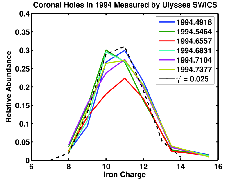
Figure 2: Observed (colored solid lines) and modeled (dashed line) Fe charge states in fast wind from polar coronal holes observed at solar minimum by Ulysses SWICS in 1994.

Figure 2 shows Fe charge states observed in the fast solar wind by Ulysses (Case 1). There are six time periods, four days in duration, identified as wind originating in the polar coronal holes during the southern polar pass. The relative abundance of the charge states for these four day periods are averaged and plotted. The distributions tend to peak between $Q_{Fe}$ = 10 - 11. This is consistent with the finding of Ko et al. (1999) for the years 1994 - 1995. A solution from the model with $\gamma^{\prime}$ = 0.025 and an initial speed at $1.05R_{\sun}$ of 10 km s^-1 (the preferred value from Laming, 2004) is shown to closely match the observed distribution function. Fe charge states for a variety of these models are given in Table 2, and $\gamma^{\prime}$ is defined in section 3. This demonstrates how lower hybrid wave damping can additionally heat the solar wind before the charge states freeze-in matching observations, and that only one characteristic density scale length is required.

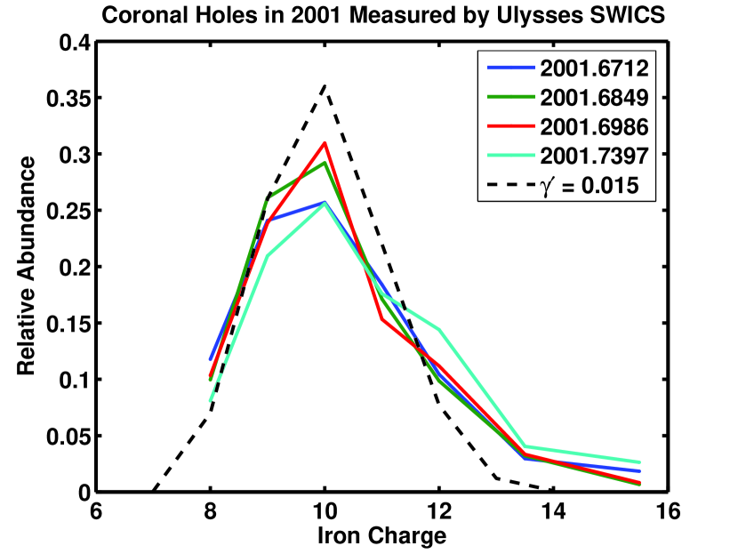
Figure 3: Observed (colored solid lines) and modeled (dashed line) Fe charge states in fast wind from polar coronal holes observed at solar maximum by Ulysses SWICS in 2001.

Figure 3 shows the Fe charge state distributions for a solar maximum coronal hole observed by Ulysses SWICS. These four four-day periods occurred during the northern polar pass toward the end of 2001. Again the charge states represent the mean charge state distribution observed during these periods. The maximum charge state for this period is near 10, although a large fraction remains in $Q_{Fe}$ = 9. These distributions are compared to a model with a heating rate of $\gamma^{\prime}$ = 0.015. However it is clear that the observed charge state distributions are broader than the model, indicating that a range of density scale lengths may be present.

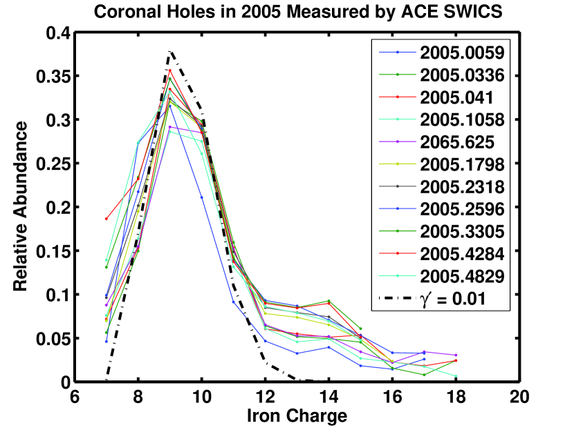
Figure 4: Observed (colored solid lines) and modeled (dashed line) Fe charge states in fast wind peaking at Q_Fe = 9 from equatorial coronal holes observed by ACE in 2005. The average charge states are lower still than the solar maximum coronal holes, and the distributions are generally broader. The $\alpha$ particle wind speed is also the lowest in these cases.

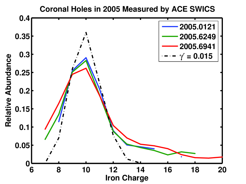
Figure 5: Observed (colored solid lines) and modeled (dashed line) Fe charge states in fast wind peaking at Q_Fe = 10 from equatorial coronal holes observed by ACE in 2005. The average charge states are lower still than the solar maximum coronal holes, and the distributions are generally broader. The $\alpha$ particle wind speed is also the lowest in these cases.

Figures 4 and 5 show the Fe charge state distribution for fast solar wind associated with an equatorial coronal hole observed by ACE SWICS during solar minimum. For these plots, 14 periods are selected ranging from 2-4 days in duration. These periods represent different passes through fast solar wind, whereas the previous two examples represent different periods within the same coronal hole. The periods are separated into those that peak at $Q_{Fe}$ = 9 (Figure 4) and those that peak near $Q_{Fe}$ = 10 (Figure 5). The charge state distributions that peak at $Q_{Fe}$ = 9 are fit best by a model $\gamma^{\prime}$ = 0.01, while the charge state distributions that peak at $Q_{Fe}$ = 10 are best fit by a model $\gamma^{\prime}$ = 0.015, which implies more heating by wave damping is needed for these. The model results fail to catch the shoulder of the charge state distributions out to a charge state of 14 and beyond.

Since the ionization model assumes solar minimum conditions over the poles, there may be additional characteristics that need to be considered for a full understanding of the contribution of wave damping for the heating of ions in different solar wind streams from coronal holes. Miralles et al. (2001) observed that the O⁵⁺ outflow speed was lower for the equatorial coronal holes than for the polar coronal holes, despite the fact that their final solar wind speeds at 1 AU are not significantly different. The wind acceleration must occur further out, possibly beyond the radii associated with freeze-in, leading to lower degrees of enhanced ionization. It may be that the higher densities in these structures prevent the plasma from becoming collisionless further from the solar surface than is the case in polar coronal holes, or that the increased magnetic field strength (Wang et al., 2000) inhibits the turbulent cascade until the field has decreased sufficiently further out, since three-wave interaction probabilities go as $\left(\omega/\Omega_{i}\right)^{4}$ (Luo & Melrose, 2006).

Ulysses charge states from the solar minimum polar coronal hole during 1994 are observed to be higher than the charge states in the solar maximum polar coronal hole observed by Ulysses in 2001. The charge states in the equatorial coronal hole observed at ACE in 2005 are even lower, with an average charge state of 9+ for Fe. The trend toward lower average charge states correlates with the average of the solar wind speeds during the periods measured. The average speed of the solar wind alpha particles observed from the solar minimum equatorial coronal hole at ACE was 650 km/s (ranging from 600 - 800 km/s) , while solar wind alpha speeds from the solar minimum polar coronal hole at Ulysses were at 800 km/s +/- 20 km/s. The wind speeds were more variable in the ACE observations. The relationship of solar wind alpha speed and mean Fe charge state and therefore lower hybrid damping rate indicates that less additional electron heating is needed in slower flows at lower latitudes. The electron temperatures required to produce the observed charge are slightly lower than was the case in Laming (2004), due to the small downwards revision of these charge states. We find the collisionless equilibration parameter $\gamma^{\prime}$ in the range 0.01 - 0.025, which corresponds to the curves labeled 0.2 - 0.5 in Figure 5 of Laming (2004). This represents a small change, becoming a little more consistent with the observational error bars from Wilhelm et al. (1998).

5 Discussion: Relation to MHD Turbulence

The cascade of Alfvénic MHD turbulence from small to large $k_{\perp}$ is expected to produce cross field variations on small length scales of density, magnetic field and velocity. Markovskii et al. (2006) consider in most detail the velocity shear produced by perpendicularly propagating Alfvénic fluctuations. Such perturbations will also produce small scale perpendicular variations in magnetic field. While magnetic curvature may also give rise to lower hybrid waves, it is the longitudinal variation that is important in this respect. However $k_{\|}$ does not cascade to large values, unlike $k_{\perp}$, so we are left with cross-field density gradients as the most effective means of generating lower hybrid waves. Significant density fluctuations cannot arise solely from Alfvénic turbulence. Waves of a compressive character such as fast mode waves are required. Luo & Melrose (2006), in an analytic consideration of three-wave processes involving two or three Alfvén waves and at most one fast mode wave, show that a critical frequency, $\omega_{c}$, exists, such that below this frequency fast mode waves dominate, and above Alfvén waves are more prevalent. In the simplest case involving one fast mode wave and two Alfvén waves, with one of the Alfvén wave frequencies, $\omega_{l}$, much lower than the other two, $\omega_{c}\sim 2\omega_{pi}^{2/3}\omega_{l}^{1/3}$, putting $W_{F}\sim W_{A}$ in their equation 25. For a density of $10^{6}$ cm^-3 and magnetic field of 1 G, $\omega_{l}\sim 0.07$ which corresponds to a wave period of 90 s, assuming that in our case, fast mode turbulence must dominate up to frequencies corresponding to the ion gyrofrequency. Waves of this period or longer are reported in coronal holes, (Ofman et al., 1999; Banerjee et al., 2001), and so the existence of fast mode turbulence would not seem to be a problem. Chandran (2005), adopting a numerical approach to consider a wider range of processes involving Alfvén and fast mode waves, finds different regions of $k$-space dominated by Alfvén or fast mode turbulence. Suzuki, Lazarian, & Beresnyak (2006) conjecture that the degree of coupling between fast modes and Alfvén modes should be reduced in strong Alfvénic turbulence; both Luo & Melrose (2006) and Chandran (2005) only consider weak Alfvénic turbulence. Slow mode waves have not been considered as part of the turbulent cascade, but Ballai et al. (2003) discuss the behavior of slow mode solitary waves, which could also produce suitable density gradients in perpendicular propagation.

Direct evidence of turbulent cascade down to these small scales has been hard to come by. However Cluster (Bale et al., 2005) has observed electric and magnetic fluctuation spectra in the solar wind near the terrestrial bowshock. In the inertial range, both spectra resemble a Kolmogorov $k^{-5/3}$ behavior. However as the dissipation range is approached, at $kr_{g}\sim 1$ where $r_{g}$ is the ion gyroradius, the magnetic spectrum steepens, while the electric spectrum flattens. Clearly the turbulence is becoming more electrostatic. Measurements of the phase speed suggest the turbulence is mainly Alfvénic in nature, transforming to kinetic Alfvén waves in the dissipation range and damping by heating the ambient plasma as the waves become more electrostatic. This is entirely consistent with the approach taken in this paper, except that the electrostatic waves we consider derive not directly from the cascading turbulence, but as a by-product of the damping.

We determine a likely order of magnitude of $\gamma^{\prime}\sim 0.01$ from charge states observed in the fast solar wind. Assuming a wave electric field given by equation A3 and a Maxwellian distribution for the $\alpha$ particles that excite the waves, we determine a density scale length $L\sim 4r_{g}$ from figure 11 in Laming (2004), where $r_{g}$ is the gyroradius of the $\alpha$ particles. Observations of $\alpha$ particles in the solar wind typically give a $\kappa$ distribution in the parallel direction with $\kappa\sim 3-6$ (Collier et al., 1996; Chotoo et al., 1998), which if it has an origin in energization by ion cyclotron waves would correspond to $\kappa\sim 3.5-6.5$ in the perpendicular direction. This would increase our density scale length estimate to $L\sim 6-10r_{g}$. We showed earlier that ion heating is negligible compared to electron heating for lower hybrid waves excited under solar wind parameters. Thus the electric field estimate in equation A3 may be exceeded by as much as an order of magnitude. Hence $\gamma^{\prime}\sim 10^{-4}$, and the density scale length becomes $L\sim 10-25r_{g}$. We have no direct knowledge of the $\alpha$ particle gyroradius. The perpendicular velocities for protons and O VI are $\sim 200$ and $\sim 300-400$ km s^-1 at a heliocentric distance of about 2 $R_{\sun}$, where the magnetic field is $\sim 1$ G and the particle density is $\sim 10^{6}$ cm^-3. The proton gyroradius is then 0.02 km, and the proton inertial length is 0.2 km. At 1 AU, the minor ions flow about an Alfvén speed faster than the protons, presumably reflecting enhanced perpendicular heating by ion cyclotron waves closer to the sun. The $\alpha$ particles also flow faster than the protons (Reisenfeld et al., 2001; von Steiger et al., 2000; Neugebauer et al., 1996), so we will assume an $\alpha$ particle perpendicular velocity of 400 km s^-1, similar to O VI. This gives an $\alpha$ particle gyroradius of 0.08 km, and the range of density scale lengths corresponds to 0.8 - 2 km, or 4 - 10 proton inertial lengths. This is very similar to the scale length of velocity shear discussed by Markovskii et al. (2006). Thus it seems that our results support ideas of turbulent cascade of MHD fluctuations in the solar wind. Other observations of density structures observed by Interplanetary Scintillation are reviewed in Laming (2004).

Another often cited mechanism for electron heating in the solar wind is the Landau damping of kinetic Alfvén waves (e.g. Cranmer & van Ballegooijen, 2003) by the small parallel component of the wave electric field. This process, and that for fast mode waves also, are considered in some detail by Vinas et al. (2000), with application to the formation of suprathermal electrons in the chromosphere. Their solution of the dispersion relation only yields significant parallel electric fields for wavevectors approaching $10c/\omega_{pi}$ for both fast mode and kinetic Alfvén waves. At $k\sim c/\omega_{pi}$, the parallel electric field is a factor $\sim 10^{-4}$ smaller than the perpendicular field, and smaller by at least an order of magnitude than the parallel electric field due to lower hybrid waves if the density gradients we infer above are related to Alfvén or fast mode wavevectors. More generally, one can estimate the parallel electric field from the expression (Hasegawa, 1976, equation 37)

$$E_{\|}=r_{g}^{2}{T_{e}\over T_{i}}\partial_{\|}\left(\partial_{\perp}E_{\perp}\right),$$ (16)

which would suggest that wavelengths of order the proton gyroradius are required. This is less restrictive than the results of Vinas et al. (2000), but still significantly more so than what we determine for lower hybrid waves. It would appear then that electron heating by kinetic Alfvén waves places even more stringent requirements on the turbulent cascade than do the lower hybrid waves. Another potential problem is that no natural means of suppressing electron heating at altitudes within 1.5 $R_{\sun}$ heliocentric distance exists, which might lead to conflict with the SUMER electron temperature observations of Wilhelm et al. (1998) and others.

6 Conclusions

We have revisited the model of Laming (2004) for increased ionization in the fast solar wind with the analysis of new data, and some refinements to the theory. The important new development, due in part to the revision downwards of charge states observed in the solar wind, and more significantly to the correction of an error in Laming (2004) in the expression for the wave energy density, is that the degree of density inhomogeneity required in the fast solar wind acceleration region to produce the required heating is now reduced from a length on the order of an ion gyroradius, to be in the range 10 - 25 gyroradii. As discussed above, this makes a connection between these density gradients and the outcome of the MHD turbulent cascade much more likely. Our finding that ion excited lower hybrid waves develop stronger parallel electric fields than kinetic Alfvén waves reinforces suggestions like that of Begelman & Chiueh (1988) that such mechanisms may have more general relevance elsewhere in astrophysics.

In our models, the appropriate choice of the electron-ion equilibration parameter can yield a fit for the observed distribution functions for various fast solar wind streams. This supports the idea that existence of density gradients from MHD turbulent cascades can allow lower hybrid waves to oscillate and damp, imparting their energy to electron heating. This electron heating due to the damping of the lower hybrid waves occurs in the region beyond $1.5R_{\sun}$, where ions begin to execute large gyro- orbits under the influence of perpendicular heating by ion cyclotron waves. The solar wind flows with the highest alpha particle speeds also have the highest average charge states, implying that the electron heating is most efficient in fast outflow from polar coronal holes during solar minimum. Lower fast wind speeds result in lower average charge states of Fe, clearly indicating a connection between electron heating and ion acceleration. Finally, in Table 3, we give predicted charge states for Ne, Mg, Si, S, Ar, and Ca, again for an initial wind speed of 10 km s^-1 at $1.05R_{\sun}$.

Appendix A Wave Trapping and Threshold Electric Field

The equation of motion for a particle in the electric field of a wave is

$${dv\over dt}={qE\over m}\exp i\psi={qE\over m}\cos\psi$$ (A1)

where $\psi=\omega t-kz$ and real parts are taken in the last step. Writing $\partial^{2}z/\partial t^{2}=-\left(1/k\right)\partial^{2}\psi/\partial t^{2}=qE/m\cos\psi$ we arrive at

$${\partial^{2}\over\partial t^{2}}{\partial\psi\over\partial t}={qEk\over m}{\partial\psi\over\partial t}\sin\psi=-\omega_{T}^{2}{\partial\psi\over\partial t}\sin\psi$$ (A2)

where $\omega_{T}=\sqrt{-qEk/m}$ is the particle trapping frequency. A particle is said to be “trapped” when $v>\left(\omega-\omega_{T}\right)/k$ during its cyclotron orbit. The time spent in the trapping region during a cyclotron orbit is $2\theta/\Omega$ where $\cos\theta=1-\omega_{T}/\omega\simeq 1-\theta^{2}/2$, so the time is $2/\Omega\times\sqrt{2\omega_{T}/\omega}$. The trapping is defined as effective when the time spent in the trapping region is $\geq 1/\omega_{T}$, so $8\omega_{T}^{3}=\Omega^{2}\omega$, which then gives

$${E_{0}\over B_{0}}={1\over 4}\left(\Omega\over\omega\right)^{1/3}{\omega\over kc},$$ (A3)

which is the result of Karney (1978), derived by integration of the Hamiltonian equations of motion.

Appendix B Electron Distributions from Lower-Hybrid Wave Heating

We write the Boltzmann equation as

$${df\over dt}={1\over v_{\perp}}{\partial\over\partial v_{\perp}}\left[v_{\perp}\left\{A_{\perp}f+\left(D_{\perp\perp}{\partial f\over\partial v_{\perp}}+D_{\perp\|}{\partial f\over\partial v_{\|}}\right)\right\}\right]+{\partial\over\partial v_{\|}}\left\{A_{\|}f+D_{\|\perp}{\partial f\over\partial v_{\perp}}+D_{\|\|}{\partial f\over\partial v_{\|}}\right\}=0,$$ (B1)

where $A_{\perp}$ and $A_{\|}$ are coefficients of dynamical friction and $D_{\perp\perp}$, $D_{\|\|}$, $D_{\perp\|}$, and $D_{\|\perp}$ are velocity diffusion coefficients. Integrating the Boltzmann equation over $v_{\perp}$ from 0 to $\infty$, we have

$${\partial\over\partial v_{\|}}\left\{A_{\|}\int f2\pi v_{\perp}dv_{\perp}+\int D_{\|\perp}{\partial f\over\partial v_{\perp}}2\pi v_{\perp}dv_{\perp}+D_{\|\|}{\partial\over\partial v_{\|}}\int f2\pi v_{\perp}dv_{\perp}\right\}=0$$ (B2)

in steady state conditions (i.e. $df/dt=0$). This integrates to

$$\int f2\pi v_{\perp}dv_{\perp}\propto\exp\left(-\int A_{\|}/D_{\|\|}dv_{\|}\right)=\exp\left(-v_{\|}^{2}/2v_{t\|}^{2}\right)$$ (B3)

when $A_{\|}=v_{\|}/\tau$, $D_{\|\perp}=v_{t\|}v_{t\perp}/\tau_{d}$ and $D_{\|\|}=v_{t\|}^{2}/\tau_{s}$, with the deflection time $\tau_{d}>>\tau_{s}$, the stopping time, $\tau_{s}=2\pi n_{e}v_{\|}^{3}/3\omega_{pe}^{4}\ln\Lambda$ for fast electrons in cold plasma, with $\ln\Lambda\sim 30$ being the Coulomb logarithm. For comparison, the electron-electron equilibration time, $t_{eq}=\sqrt{2/3}\pi^{3/2}n_{e}v^{3}/\omega_{pe}^{4}\ln\Lambda$, is a factor of a few higher.

For electron heating by Landau damping, the non-zero diffusion coefficient and coefficient of dynamical friction are (Melrose, 1986, equation 10.83 and 10.90 with $s=0$)

$$D_{\|\|} =\int{8\pi^{2}q^{2}\over\hbar}{R\over\omega}\left|\vec{e}\cdot\vec{V}\right|^{2}\delta\left(\omega-k_{\|}v_{\|}\right)\left(\hbar k_{\|}\over m\right)^{2}N{d^{3}k\over\left(2\pi\right)^{3}}$$ (B4)

$$A_{\|} =\int{8\pi^{2}q^{2}\over\hbar}{R\over\omega}\left|\vec{e}\cdot\vec{V}\right|^{2}\delta\left(\omega-k_{\|}v_{\|}\right)\left(\hbar k_{\|}\over m\right){d^{3}k\over\left(2\pi\right)^{3}},$$ (B5)

where in the small gyroradius limit $\vec{V}=\left(0,0,v_{\|}\right)$ and $\vec{e}$ is the wave polarization vector. The number density of wave quanta is given by $N$, $R$ is the ratio of electric energy to total energy in the wave, such that $R\int N\hbar\omega d^{3}k/\left(2\pi\right)^{3}=\delta E^{2}/8\pi$. For lower hybrid waves

$$K^{L}=1+{\omega_{pe}^{2}\over\Omega_{e}^{2}}\sin^{2}\theta-{\omega_{pe}^{2}\over\omega^{2}}+{\omega_{pi}^{2}\over kv_{i}^{2}}\left(1-\phi\left(\omega\over\sqrt{2}kv_{i}\right)\right)$$ (B6)

where $\phi\left(x\right)$ is the usual plasma dispersion function and $v_{i}=\sqrt{k_{B}T_{i}/m_{i}}$ is the ion thermal velocity. We consider two possibilities. When $\omega>>\sqrt{2}kv_{i}$, $\phi\simeq 1-k^{2}v_{i}^{2}/\omega^{2}$ and

$$\omega^{2}={\omega_{pi}^{2}+\omega_{pe}^{2}\cos^{2}\theta\over 1+\omega_{pe}^{2}\sin^{2}\theta/\Omega_{e}^{2}},$$ (B7)

and when $\omega<<\sqrt{2}kv_{i}$, $\phi\simeq\omega^{2}/k^{2}v_{i}^{2}$, and

$$\omega^{2}={\omega_{pe}^{2}\cos^{2}\theta\over 1+\omega_{pe}^{2}\sin^{2}\theta/\Omega_{e}^{2}+\omega_{pi}^{2}/k^{2}v_{i}^{2}}.$$ (B8)

In either case, the ratio of electric to total energy in the wave $R=\left(\omega\partial\Re K^{L}/\partial\omega\right)^{-1}\sim\Omega_{e}^{2}/2\omega_{pe}^{2}$ and $\left|\vec{e}\cdot\vec{V}\right|^{2}=v_{\|}^{2}\cos^{2}\theta$. For $\omega<<\sqrt{2}kv_{i}$, both $\omega$ and the growth rate $\gamma$ vary as $\cos^{2}\theta$. Consequently wave generation will occur mainly at $\cos\theta=\omega_{pi}/\omega_{pe}$, beyond which lower hybrid waves are progressively Landau damped by parallel propagating electrons. This then yields

$$D_{\|\|} =\pi{\partial\over\partial k_{\|}}\left(q\delta E\over m_{e}\right)^{2}{\omega_{pi}^{2}\over\omega_{pe}^{2}v_{\|}}$$ (B9)

$$A_{\|} ={\omega_{pi}^{2}\Omega_{e}^{4}\over 8\pi\omega_{pe}^{2}n_{e}v_{te\perp}^{2}}$$ (B10)

where $\partial/\partial k_{\|}\left(q\delta E/m_{e}\right)^{2}$ is evaluated at $k_{\|}=\omega/v_{\|}$. For all cases of interest, $A_{\|}<<v_{\|}/\tau$ and so

$$f\sim\exp\left(-\int v_{\|}/\left[v_{t\|}^{2}+\tau D_{\|\|}\right]dv_{\|}\right)=\left[v_{t\|}^{2}+v_{\|}^{2}/2\kappa\right]^{-\kappa},$$ (B11)

where $\kappa=\left[4\pi\partial/\partial k_{\|}\left(q\delta E/m_{e}\right)^{2}\times\pi\omega_{pi}^{2}n_{e}/3\omega_{pe}^{6}\ln\Lambda\right]^{-1}$. We have assumed that $\partial/\partial k_{\|}\left(q\delta E/m_{e}\right)^{2}$ is independent of $k_{\|}$ at $\omega/v_{\|}$ and hence that $D_{\|\|}\propto 1/v_{\|}$ in the final step.

Where $\omega>>\sqrt{2}kv_{i}$, both $\omega$ and $\gamma$ remain non-zero as $\cos\theta\rightarrow 0$, so wave generation occurs for all $\cos\theta$ in the range $-\omega_{pi}/\omega_{pe}\rightarrow\omega_{pi}/\omega_{pe}$. In this case then

$$D_{\|\|} =\pi{\partial\over\partial k_{\|}}\left(q\delta E\over m_{e}\right)^{2}{\omega^{2}\over k^{2}v_{\|}^{3}}$$ (B12)

$$A_{\|} ={\omega^{2}\Omega_{e}^{4}\over 8\pi k^{2}v_{\|}^{2}n_{e}v_{te\perp}^{2}}$$ (B13)

and the electron distribution function integrates to a Maxwellian

$$f\left(v_{\|}\right) \propto\exp\left(-v_{\|}^{2}/2/\left(v_{t\|}^{2}+\left(\pi n_{e}\omega^{2}/6\omega_{pe}^{4}\ln\Lambda k^{2}\right)4\pi\partial/\partial k_{\|}\left(q\delta E/m_{e}\right)^{2}\right)\right)$$ (B14)

$$=\exp\left(-v_{\|}^{2}/2/\left(v_{t\|}^{2}+\left(\omega^{2}/k^{2}v_{\|}^{2}\right)\left(\tau_{s}\pi/v_{\|}\right)\partial/\partial k_{\|}\left(q\delta E/m_{e}\right)^{2}\right)\right).$$

We also estimate $A_{\|}\simeq 10^{11}/n_{e}<<v_{\|}/\tau_{s}$ as required with $B=10$G.

Appendix C Atomic Data Updates

We have also updated the atomic data for dielectronic recombination of K-shell, and L-shell ions. Recombination from H- to He-like and from He- to Li-like are taken from Dasgupta & Whitney (2004). The successive isoelectronic sequences Li-, Be-, B-, C-, N-, O-, and F-like are taken from Colgan, Pindzola, & Badnell (2004), Colgan et al. (2003), Altun et al. (2004), Zatsarinny et al. (2004a), Mitnik & Badnell (2004), Zatsarinny et al. (2003), and Gu (2003) respectively. Additionally dielelectronic recombination from Ne- to Na-like and from Na- to Mg-like are taken from Zatsarinny et al. (2004b) and Gu (2004).

Table 1: O⁺⁶/O⁺⁷ Abundance Ratios

$v_{start}$ (km s-1)	$\gamma^{\prime}$	$\kappa_{min}$	O+6/O+7	O+6/O${}^{+7}_{\kappa\rightarrow\infty}$
5	0.005	4.00	310	360
	0.01	3.40	247	205
	0.02	3.07	156	79
	0.03	2.95	115	50
	0.04	2.89	95	38
	0.05	2.84	84	32
	0.06	2.82	74	28
	0.08	2.78	65	24
	0.1	2.75	58	22
10	0.005	4.78	278	328
	0.01	3.78	192	145
	0.02	3.29	89	46
	0.03	3.12	59	27
	0.04	3.03	46	21
	0.05	2.97	38	17
	0.06	2.93	34	15
	0.08	2.87	29	13
	0.1	2.84	26	11
20	0.005	5.92	221	278
	0.01	4.38	118	99
	0.02	3.62	46	26
	0.03	3.36	27	15
	0.04	3.23	21	11
	0.05	3.14	17	9
	0.06	3.08	15	9
	0.08	3.00	12	7
	0.1	2.96	11	6
Geiss et al. (1995)				30
Ko et al. (1997)				32

Table 2: Fe Charge State Fractions

$v_{start}$ (km s-1)	$\gamma^{\prime}$	Fe+7	Fe+8	Fe+9	Fe+10	Fe+11	Fe+12	Fe+13	Fe+14
	0.0	0.21	0.63	0.094	0.025	0.0044	0.0004
	0.005	0.041	0.60	0.29	0.059	0.006	0.0004
	0.007	0.019	0.49	0.37	0.11	0.015	0.001
	0.01	0.007	0.34	0.42	0.19	0.039	0.005	0.0002
	0.015	0.003	0.20	0.40	0.28	0.093	0.017	0.001
	0.02	0.0012	0.14	0.35	0.33	0.14	0.035	0.004	0.0003
	0.025	0.0007	0.10	0.31	0.35	0.18	0.054	0.007	0.0007
	0.03	0.0005	0.076	0.28	0.35	0.21	0.073	0.012	0.001
	0.04	0.0003	0.052	0.23	0.35	0.25	0.10	0.021	0.003
	0.05	0.0002	0.040	0.20	0.34	0.27	0.13	0.029	0.004
	0.06	0.0001	0.032	0.17	0.32	0.28	0.15	0.036	0.006
	0.08		0.024	0.15	0.31	0.30	0.17	0.047	0.008
10	0.0	0.17	0.62	0.13	0.043	0.009
	0.005	0.020	0.47	0.37	0.12	0.017	0.0013
	0.007	0.0075	0.32	0.42	0.21	0.047	0.006
	0.01	0.0023	0.17	0.38	0.31	0.11	0.022	0.002
	0.015	0.0005	0.070	0.26	0.36	0.22	0.077	0.012	0.001
	0.02		0.035	0.18	0.33	0.28	0.14	0.030	0.004
	0.025		0.020	0.13	0.29	0.31	0.19	0.052	0.009
	0.03		0.013	0.097	0.26	0.31	0.23	0.074	0.015
	0.04		0.006	0.062	0.20	0.31	0.28	0.11	0.029
	0.05		0.004	0.044	0.17	0.29	0.30	0.14	0.043
	0.06		0.003	0.034	0.14	0.27	0.32	0.17	0.055
	0.08		0.002	0.023	0.11	0.24	0.33	0.20	0.074
20	0.0	0.14	0.58	0.18	0.074	0.020	0.003
	0.005	0.003	0.13	0.31	0.34	0.17	0.047	0.007	0.0002
	0.007	0.0008	0.057	0.22	0.35	0.26	0.10	0.016	0.0013
	0.01	0.0001	0.016	0.10	0.27	0.32	0.22	0.062	0.010
	0.015		0.0039	0.041	0.16	0.29	0.32	0.14	0.038
	0.02		0.0013	0.019	0.099	0.24	0.34	0.21	0.077
	0.025		0.002	0.023	0.11	0.25	0.34	0.19	0.069
	0.03		0.0008	0.013	0.076	0.20	0.34	0.24	0.10
	0.04		0.0002	0.005	0.042	0.14	0.31	0.28	0.16
	0.05		0.0001	0.003	0.026	0.10	0.28	0.30	0.20
	0.06			0.002	0.018	0.082	0.25	0.30	0.22
	0.08			0.001	0.011	0.057	0.21	0.29	0.25

Table 3: Minor Ion Charge State Fractions, $v_{start}=10$ km s^-1

element	$\gamma^{\prime}$	+5	+6	+7	+8	+9	+10	+11	+12
Ne	0.01	0.0017	0.032	0.12	0.84	0.0003
	0.015	0.0005	0.024	0.12	0.85	0.001
	0.025	0.0002	0.017	0.12	0.86	0.004
Mg	0.01	0.008	0.12	0.40	0.35	0.084	0.038
	0.015	0.004	0.089	0.38	0.40	0.095	0.036
	0.025	0.002	0.058	0.33	0.45	0.123	0.036
Si	0.01	0.004	0.12	0.47	0.34	0.070	0.004
	0.015	0.001	0.058	0.38	0.42	0.13	0.013
	0.025	0.0002	0.022	0.26	0.45	0.23	0.037	0.002
S	0.01	0.0004	0.089	0.42	0.39	0.095	0.007	0.0002
	0.015	0.0001	0.047	0.33	0.44	0.16	0.020	0.0009
	0.025		0.017	0.21	0.44	0.28	0.058	0.005
Ar	0.01			0.006	0.69	0.28	0.032	0.0013
	0.015			0.003	0.59	0.34	0.058	0.004
	0.025			0.0013	0.43	0.43	0.13	0.015	0.0007
Ca	0.01			0.005	0.034	0.10	0.81	0.048	0.0008
	0.015			0.002	0.016	0.084	0.80	0.095	0.004
	0.025			0.0003	0.004	0.045	0.75	0.18	0.015

Figure 1: Approximate (narrow solid line, from equation 12) and true (wide solid line) $\kappa$ distributions for varying $\kappa$. The underlying Maxwellian is shown in each case as a dashed line.

References

- Abramovitz & Stegun (1970) Abramowitz, M., & Stegun, I. 1970, Handbook of Mathematical Functions, (Dover Publications: New York)
- Altun et al. (2004) Altun, Z., Yumak, A., Badnell, N. R., Colgan, J., & Pindzola, M. S. 2004, A&A, 420, 775
- Bale et al. (2005) Bale, S. D., Kellogg, P. J., Mozer, F. S., Horbury, T. S., & Reme, H. 2005, Phys. Rev. Lett., 94, 215002
- Ballai et al. (2003) Ballai, I., Thelen, J. C., & Roberts, B. 2003, A&A, 404, 701
- Banerjee et al. (2001) Banerjee, D., O’Shea, E., Doyle, J. G., & Goossens, M. 2001, A&A, 380, L39
- Begelman & Chiueh (1988) Begelman, M. C., & Chiueh, T. 1988, ApJ, 332, 872
- Brambilla (1998) Brambilla, M. 1998, Kinetic Theory of Plasma Waves. Homogeneous Plasmas, (Oxford University Press: Oxford)
- Bryans et al. (2006) Bryans, P., Badnell, N. R., Gorczyca, T. W., Laming, J. M., Mitthumsiri, W., & Savin, D. W. 2006, ApJS, 167, 343
- Chandran (2005) Chandran, B. D. G. 2005, Phys. Rev. Lett., 95, 265004
- Chotoo et al. (1998) Chotoo, K., Collier, M. R., Galvin, A. B., Hamilton, D. C., & Gloeckler, G. 1998, J. Geophys. Res., 103, 17441
- Colgan et al. (2003) Colgan, J., Pindzola, M. S., Whiteford, A. D., & Badnell, N. R. 2003, A&A, 412, 597
- Colgan, Pindzola, & Badnell (2004) Colgan, J., Pindzola, M. S., & Badnell, N. R. 2004, A&A, 417, 1183
- Collier et al. (1996) Collier, M. R., Hamilton, D. C., Gloeckler, G., Bochsler, P., & Sheldon, R. B. 1996, Geophys. Res. Lett., 23, 1191
- Cranmer et al. (1999a) Cranmer, S. R., et al. 1999, ApJ, 511, 481
- Cranmer et al. (1999b) Cranmer, S. R., Field, G. B., & Kohl, J. L. 1999, ApJ, 518, 937
- Cranmer (2000) Cranmer, S. R. 2000, ApJ, 532, 1197
- Cranmer & van Ballegooijen (2003) Cranmer, S. R., & van Ballegooijen, A. A. 2003, ApJ, 594, 573
- Dasgupta & Whitney (2004) Dasgutpa, A., & Whitney, K. G. 2004, PRA, 69, 022702
- Esser & Edgar (2000) Esser, R., & Edgar, R. J. 2000, ApJ, 532, L71
- Geiss et al. (1995) Geiss, J., et al. 1995, Science, 268, 1033
- Gradshteyn & Ryzik (1994) Gradshteyn, I. S., & Ryzik, I. M. 1994, Tables of Integrals, Series, and Products, (Academic Press: New York)
- Gu (2003) Gu, M. F. 2003, ApJ, 590, 1131
- Gu (2004) Gu, M. F. 2004, ApJS, 153, 389
- Hasegawa (1976) Hasegawa, A. 1976, J. Geophys. Res., 81, 5083
- Karney (1978) Karney, C. F. F. 1978, Phys. Fluids, 21, 1584
- Karney (1979) Karney, C. F. F. 1979, Phys. Fluids, 22, 2188
- Ko et al. (1997) Ko, Y.-K., Kisk, L. A., Geiss, J., Gloeckler, G. A., & Guhathakurta, M. 1997, Sol. Phys., 171, 345
- Ko et al. (1999) Ko, Y.-K., Gloeckler, G., Cohen, C. M. S., & Galvin, A. B. 1999, J. Geophys. Res., 104, 17,005
- Laming (2004) Laming, J. M. 2004, ApJ, 604, 874
- Laming (2001) Laming, J. M. 2001, ApJ, 546, 1149
- Luo & Melrose (2006) Luo, Q., & Melrose, D. 2006, MNRAS, 368, 1151
- Maksimovic et al. (2000) Maksimovic, M., Gary, S. P., & Skoug, R. M. 2000, J. Geophys. Res., 105, 18,337
- Markovskii et al. (2006) Markovskii, S. A., Vasquez, B. J., Smith, C. J., & Hollweg, J. V. 2006, ApJ, 639, 1177
- Markovskii & Hollweg (2002) Markovskii, S. A., & Hollweg, J. V. 2002, J. Geophys. Res., 107, SSH 21-1
- Markovskii (2001) Markovskii, S. A. 2001, ApJ, 557, 337
- Mazzotta et al. (1998) Mazzotta, P., Mazzitelli, G., Colafrancesco, S., & Vittorio, N. 1998, A&AS, 133, 403
- Melrose (1986) Melrose, D. B. 1986, Instabilities in Space and Laboratory Plasmas, (Cambridge University Press: Cambridge)
- Miralles et al. (2001) Miralles, M. P., Cranmer, S. R., Panasyuk, A. V., Romoli, M., & Kohl, J. L. 2001, ApJ, 549, L257
- Mitnik & Badnell (2004) Mitnik, D. M., & Badnell, N. R. 2004, A&A, 425, 1153
- Neugebauer et al. (1996) Neugebauer, M., Goldstein, B. E., Smith, E. J., & Feldman, W. C. 1996, J. Geophys. Res., 101, 17047
- Ofman et al. (1999) Ofman, L., Nakariakov, V. M., & DeForest, C. E. 1999, ApJ, 514, 441
- Reisenfeld et al. (2001) Reisenfeld, D. B., Gary, S. P., Gosling, J. T., Steinberg, J. T., McComas, D. J., Goldstein, B. E., & Neugebauer, M. 2001, J. Geophys. Res., 106, 5693
- Suzuki, Lazarian, & Beresnyak (2006) Suzuki, T. K., Lazarian, A., & Beresnyak, A. 2006, ApJ, submitted, astro-ph/0608307
- Vinas et al. (2000) Vinas, A. F., Wong, H. K., & Klimas, A. J. 2000, ApJ, 528, 509
- Vocks et al. (2005) Vocks, C., Salem, C., Lin, R. P., & Mann, G. 2005, ApJ, 627, 540
- von Steiger et al. (2000) von Steiger, R., et al. 2000, J. Geophys. Res., 105, 27217
- Wang et al. (2000) Wang, Y.-M., Lean, J., & Sheeley, N. R. 2000, Geophys. Res. Lett.,27, 505
- Wilhelm et al. (1998) Wilhelm, K., Marsch, E., Dwivedi, B, Hassler, D. M., Lemaire, P., Gabriel, A. H., & Huber, M. C. E. 1998, ApJ, 500, 1023
- Zatsarinny et al. (2004a) Zatsarinny, O., Gorczyca, T. W., Korista, K. T., Badnell, N. R., & Savin. D. W. 2004, A&A, 417, 1173
- Zatsarinny et al. (2003) Zatsarinny, O., Gorczyca, T. W., Korista, K. T., Badnell, N. R., & Savin. D. W. 2003, A&A, 412, 587
- Zatsarinny et al. (2004b) Zatsarinny, O., Gorczyca, T. W., Korista, K. T., Badnell, N. R., & Savin. D. W. 2004, A&A, 426, 699