Validating a Time-Dependent Turbulence-Driven Model of the Solar Wind

Abstract

Although the mechanisms responsible for heating the Sun’s corona and accelerating the solar wind are still being actively investigated, it is largely accepted that photospheric motions provide the energy source and that the magnetic field must play a key role in the process. Verdini et al. (2010) presented a model for heating and accelerating the solar wind based on the turbulent dissipation of Alfvén waves. We first use a time-dependent model of the solar wind to reproduce one of Verdini et al.’s solutions; then we extend its application to the case when the energy equation includes thermal conduction and radiation losses, and the upper chromosphere is part of the computational domain. Using this model, we explore parameter space and describe the characteristics of a fast-solar-wind solution. We discuss how this formulation may be applied to a 3D MHD model of the corona and solar wind (Lionello et al., 2009).

1 INTRODUCTION

The identification of the physical processes responsible for the heating of the solar corona and the acceleration of the solar wind still represents an unsolved problem in solar physics. However, there is a general consensus that photospheric motions provide the energy source and that the magnetic field must play a key role in the process. Since it is clear that the measured speeds of fast streams require an extended heating deposition (Withbroe & Noyes, 1977; Holzer & Leer, 1980; Withbroe, 1988), previous one-dimensional (1D) models generally relied on a parametric heating function exponentially decaying with height (Hammer, 1982a, b; Withbroe, 1988; Hansteen & Leer, 1995; Habbal et al., 1995; Hansteen et al., 1997). At the same time, several investigations were based on low-frequency broadband fluctuations on magnetohydrodynamic scales as the mechanism that heats and accelerates the solar wind (Coleman, 1968; Belcher & Davis, 1971; Hollweg, 1986; Hollweg & Johnson, 1988; Velli, 1994; Matthaeus et al., 1999; Verdini & Velli, 2007; Zank et al., 2012).

Connecting the macroscopic heating of the plasma and acceleration of the wind, as formulated in coronal and inner heliospheric MHD models, with the underlying physical mechanisms is complicated due to the temporal and spatial dynamic ranges involved. In the past decade, turbulent dissipation mechanisms have been progressively incorporated with various degrees of self-consistency into 1D models of the solar wind (Suzuki & Inutsuka, 2005; Cranmer & van Ballegooijen, 2005; Cranmer et al., 2007; Cranmer, 2010; Verdini et al., 2010; Chandran et al., 2011). There are also efforts to replace empirical heating functions in three-dimensional (3D) MHD models with some form of turbulence dissipation mechanism. This is particularly challenging because such 3D models would have to resolve time-scales extending from a millisecond (dissipative time-scale in the solar corona) up to many days (large scale solar wind stream structure). van der Holst et al. (2010) introduced, beside the acceleration of the solar wind through Alfvén waves, the heating of the protons by Kolmogorov dissipation in open field-line regions. Usmanov et al. (2011) developed a large-scale MHD heliospheric model with small-scale transport equations for the turbulence energy, normalized cross helicity, and correlation scale, applicable where the solar wind is already supersonic and superalfvénic. The model of Lionello et al. (2013) included the effect of outwardly propagating Alfvénic turbulence in the solar wind and a phenomenological term to describe nonlinear interactions associated with wave reflection by density gradients in the chromosphere and corona. Sokolov et al. (2013) and introduced Alfvén wave turbulence, assuming that this turbulence and its nonlinear dissipation are the only momentum and energy source for heating the coronal plasma and driving the solar wind (see van der Holst et al., 2013, for additional details).

The present work illustrates the integration of the turbulence dissipation heating and acceleration mechanism of Verdini et al. (2010) in a time-dependent, 1D, hydrodynamic (HD) model of the solar wind, which includes also thermal conduction and radiation losses. In this early, explorative phase, it is expedient to conduct an investigation using 1D models so that we may later apply our gained experience to 3D models. The model of Verdini et al. (2010) employs strong turbulence closure to treat nonlinear effects, and does not rely on electron heat conduction for radial energy transport, but rather computes the internal energy associated with protons only. After presenting the characteristics of our turbulence-driven HD model, we show how it can match one of the solutions derived by Verdini et al. (2010) without thermal conduction and radiation losses. Subsequently, we extend the application of our model to include transport mechanisms in the energy equation, which are necessary to reproduce plasma emission in agreement with observations (Lionello et al., 2009). Our exploration of parameter space yields solutions compatible with the solar wind properties obtained from in situ measurements and observations. In the future we plan to introduce this formulation into the 3D MHD thermodynamic model of the solar corona and solar wind of Lionello et al. (2009).

This paper is organized as follows: the equations and the solution technique are described in Sec. 2. In Sec. 3 we present a solution in the configuration of Verdini et al. (2010), we conduct a parameter study that includes thermal conduction and radiative losses, and we describe the details of one of the solutions. We conclude with a discussion.

2 MODEL DESCRIPTION

Verdini et al. (2010) solved a steady-state, 1D model of the solar wind along an expanding flux tube that included heating and acceleration from turbulent dissipation. We solve a more general set of time-dependent, 1D HD equations along an open magnetic field line that can be reduced to the model of Verdini et al. (2010) as a special case:

$$\frac{\partial\rho}{\partial t} = -\frac{1}{A}\frac{\partial}{\partial s}\left(AU\rho\right),$$ (1)

$$\rho\frac{\partial U}{\partial t} = -\rho U\frac{\partial U}{\partial s}-\frac{\partial}{\partial s}(p+p_{w})+g_{s}\rho+\mathrm{R}_{s}+\frac{1}{s^{2}}\frac{\partial}{\partial s}\left(s^{2}\nu\rho\frac{\partial U}{\partial s}\right),$$ (2)

$$\frac{\partial T}{\partial t} = -U\frac{\partial T}{\partial s}-(\gamma-1)\left(T{\frac{1}{A}\frac{\partial}{\partial s}A}U-\frac{m_{p}}{2k\rho}\left({\frac{1}{A}\frac{\partial}{\partial s}A}q-n_{e}n_{p}{Q(T)}+{H}\right)\right),$$ (3)

where $s\geq R_{\odot}$ is the distance along a magnetic field line, which may differ from the radial distance from the surface, $r$; $\rho$, $U$, $p=2nkT$, and $T$ are the plasma mass density, velocity, pressure, and temperature ($k$ is Boltzmann constant and $n$ the number density); $g_{s}=g_{0}R_{\sun}^{2}\mathbf{\hat{b}\cdot\hat{r}}/r^{2}$ is the gravitational acceleration along the direction of the field line ($\mathbf{\hat{b}}$), and $\nu$ is the kinematic viscosity. $A(s)=1/B(s)$ is the area factor, i.e., the inverse of the magnetic field magnitude $B(s)$, along the field line. $R_{\mathrm{s}}$ is the field aligned component of the vector divergence of the MHD Reynolds stress, $\mathbf{R}=(\delta\mathbf{b}\delta\mathbf{b}/4\pi-\rho\delta\mathbf{u}\delta\mathbf{u})$, where $\delta\mathbf{b},\delta\mathbf{u}$ are respectively the fluctuations of the magnetic field, $\mathbf{B}=B(s)\mathbf{\hat{b}}+\delta\mathbf{b}$ and velocity $\mathbf{u}=U(s)\mathbf{\hat{b}}+\delta\mathbf{u}$, with $\mathbf{\hat{b}}\cdot\delta\mathbf{b}=0=\mathbf{\hat{b}}\cdot\delta\mathbf{u}$. The wave pressure term is $p_{w}={\delta\mathbf{b}^{2}}/{8\pi}$. This form of the equations is correct for incompressible fluctuations in planes orthogonal to the density gradients, and though written somewhat differently corresponds to the equation originally derived in Heinemann & Olbert (1980) and discussed in detail, from the linear point of view, in Velli (1993). Equation (3) contains the radiation loss function $Q(T)$ as in Athay (1986), $n_{e}$ and $n_{p}$ are the electron and proton number density (which are equal for a hydrogen plasma), $\gamma=5/3$ is the polytropic index, ${q}$ is the heat flux. A collisional (Spitzer’s law) or collisionless (Hollweg, 1978) formulation is used according to the radial distance,

$${q}=\left\{\begin{array}[]{ll}\displaystyle-\kappa_{0}T^{5/2}\frac{\partial T}{\partial s}&\mbox{if $R_{\odot}\leq r\lesssim 10R_{\odot}$}\\ \alpha n_{e}kTU&\mbox{if $r\gtrsim 10R_{\odot}$}\end{array}\right.,$$ (4)

where $\kappa_{0}=9\times 10^{-7}$ erg K^-7/2 cm^-1 s^-1 and $\alpha$ is a parameter, which is set to 1. The transition between the two forms occurs smoothly at a distance of $10R_{\odot}$ from the Sun (Mikić et al., 1999), approximately where the radial electron mean free path becomes equal to the radial “trapping distance” (Hollweg, 1976, 1978). To write an expression for the heating function per unit volume $H$, which depends on the perturbations (de Karman & Howarth, 1938; Matthaeus et al., 2004), it is more convenient to use the Elsasser variables $\mathbf{z}_{\pm}=\delta\mathbf{u}\mp\delta\mathbf{b}/\sqrt{4\pi\rho}$ (Dmitruk et al., 2001). $\mathbf{z}_{+}$ ($\mathbf{z}_{-}$) represents an outward (inward) propagating perturbation along a radially outward magnetic field line. We shall assume that the actual direction of $\mathbf{z}_{\pm}$ is not important, as long as it is in the plane perpendicular to $\mathbf{\hat{b}}$ and that only low-frequency perturbations are relevant for the heating and acceleration of the solar wind. Hence, we write the incompressible, volumetric heating (Dobrowolny et al., 1980; Grappin et al., 1983; Hossain et al., 1995; Matthaeus et al., 2004) in terms of $z_{\pm}$, the Fourier components in the zero-frequency limit, as

$$H=\rho\frac{|z_{-}|z_{+}^{2}+|z_{+}|z_{-}^{2}}{4\lambda_{\perp}}.$$ (5)

Here $\lambda_{\perp}$ is the correlation scale of the turbulence, which we assume to be related to its value at the solar surface, $\lambda_{\odot}$, according to the following formula:

$$\lambda_{\perp}=\lambda_{\odot}\sqrt{\frac{A}{A_{\odot}}},$$ (6)

where $A_{\odot}$ is the flux tube area at $r=R_{\odot}$.

The evolution of $z_{\pm}$ is described by the following equations (Verdini & Velli, 2007):

$$\frac{\partial z_{\pm}}{\partial t} = -[U\pm V_{a}]\frac{\partial z_{\pm}}{\partial s}+R_{1}^{\pm}z_{\pm}+R_{2}^{\pm}z_{\mp}-\frac{|z_{\mp}|z_{\pm}}{2\lambda_{\perp}},$$ (7)

$$R_{1}^{\pm} = -\frac{1}{2}[U\mp V_{a}]\left(\frac{\partial\log V_{a}}{\partial s}+\frac{\partial\log A}{\partial s}\right),$$ (8)

$$R_{2}^{\pm} = \frac{1}{2}[U\mp V_{a}]\frac{\partial\log V_{a}}{\partial s},$$ (9)

where $V_{a}(s)=B/\sqrt{4\pi\rho}$ is the Alfvén speed along the field line. $R_{1}^{\pm}$ and $R_{2}^{\pm}$ are respectively the WKB and reflection terms related to the large scale gradients. This equation is time-dependent so a clarification is in order. Generally speaking, the linear terms in this equation are correct for Alfvén waves of any frequency. However the nonlinear damping term, which is consistent with conservation of energy together with the form (5) for the heating, is really a dimensional estimation of the full non-linear cascade rate (including wave-vector components in the perpendicular directions). For any energy spectrum which is a decreasing power -law with frequency, it is the energy in the lowest frequencies which dominates the cascade rate, and one can then remove averages involved in obtaining the cascade rate and heating function as long as the fluctuations have frequencies which are small. If one had finite frequency fluctuations, a little more caution would be required, as the heating terms in Eq. (5) would involve time-averages of the quadratic fluctuating quantities and the absolute value would be replaced by the square root of the average squared fluctuation, and also in Eq. (7) one should replace the absolute value of the opposite Elsasser variable again with the square root of the average squared quantity, as discussed in Verdini et al. (2010).

The form of scaling for $\lambda_{\perp}$ in Eq. (5) is a common assumption in the literature. We use it instead of more sophisticated expressions (e.g. Breech et al., 2008) because, in future 3D applications, it will not require us to integrate along magnetic field lines. Furthermore, more complicated formulations introduce only a second-order correction in the evolution of $z_{\pm}$ in the average of the opposite Elsasser variable would appear in the nonlinear transport term Eq. (7) rather than more physics. We can now express both $p_{w}$ and $\mathrm{R}_{s}$ in terms of $z_{\pm}$ as (Usmanov et al., 2011, 2012)

$$p_{w} = \rho\frac{(z_{-}-z_{+})^{2}}{8},$$ (10)

$$\mathrm{R}_{s} = \rho\frac{z_{+}z_{-}}{2}\frac{\partial\log A}{\partial s}.$$ (11)

The equations to be solved are quasi-hyperbolic (i.e, some of the eigenvalues coincide in certain limits, e.g. Goedbloed et al., 2010, p. 413), so at the Sun, where the solar wind is subsonic, only density and temperature can be specified, while the velocity is determined determined by solving the gas characteristic equations. At the upper radial boundary, which is placed beyond all critical points, the characteristic equations are used as well. The $z_{\pm}$ equations are also hyperbolic, and the solar wind is sub-Alfvénic at the inner boundary, so we can impose only the amplitude of the outward-propagating (from the Sun) wave. Nonuniform meshes can be specified to concentrate the resolution in the transition region, where large gradients are present. The use of a semi-implicit treatment of the Alfvén and magnetosonic waves in the momentum equation, Eq. (2), allows us to specify time steps larger than the CFL limit (Lionello et al., 1998, 1999). The special treatment of the thermal conduction and radiation loss function, as explained in Lionello et al. (2009), is used to lower the gradients in the transition region without significantly affecting the coronal solution.

We express the area factor $A(s)$ in terms of $f(s)=A(s)/s^{2}$, where the expansion factor (Kopp & Holzer, 1976) is

$$f(s) = \frac{f_{\mathrm{max}}+f_{1}\exp[-(s-r_{f})/\sigma]}{1+\exp[-(s-r_{f})/\sigma]},$$ (12)

$$f_{1} = 1-(f_{\mathrm{max}}-1)\exp[(1-r_{f})/\sigma].$$

In the present work we consider a radial field line (i.e., $s=r$) with the same parameters as those used by Verdini et al. (2010), namely $f_{\mathrm{max}}=12.5$, $r_{f}=1.31~{}R_{\odot}$, and $\sigma=0.51~{}R_{\odot}$. The magnetic field magnitude at 1 AU is $B=3\times 10^{-5}~{}G$.

3 RESULTS

Here we present applications of the model described in Sec. 2. We first perform a calculation without thermal conduction and radiative losses to recover a solution as in Verdini et al. (2010). Then we extend the model by including energy transport mechanisms in the energy equation, we complete a parameter study, and show the characteristics of a fast solar wind solution.

3.1 A Solar Wind Solution After Verdini et al. (2010)

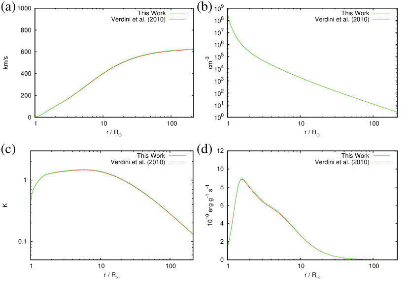
Figure 1: Comparison between the solution obtained with the model described in this work and that obtained with the model of Verdini et al. (2010): (a) wind speed; (b) density; (c) temperature; (d) total heating per unit mass. The discrepancies are less than $1\%$.

We now apply the model described in the previous section to obtain a solar wind solution with the same parameters used in Verdini et al. (2010). The model of Verdini et al. (2010) has neither thermal conduction nor radiation losses but adds instead a small compressional heating term in the lower corona:

$$\frac{H_{c}}{\rho}=3\times 10^{10}\exp\left(-\frac{\left(r/R_{\odot}-x_{g}\right)^{2}}{2\sigma_{g}^{2}}\right)~{}\mathrm{cm}^{2}\mathrm{s}^{-3},$$ (13)

with $x_{g}=1.3$, $\sigma_{g}=0.5$. The boundary conditions at the base are $T_{\odot}=4\times 10^{5}~{}\mathrm{K}$, $n_{\odot}=5\times 10^{8}~{}\mathrm{cm}^{-3}$. Among the different solutions calculated by Verdini et al. (2010), we consider the one that has $\lambda_{\odot}=0.015~{}R_{\odot}$, $z_{+}^{\odot}=37.24~{}\mathrm{km/s}$ at the solar surface, which yields a velocity perturbation $\delta u_{\odot}=20~{}\mathrm{km/s}$. A nonuniform mesh is employed with 1705 points and $\Delta s$ ranging from $7.8\times 10^{-4}~{}R_{\odot}$ at the solar surface to $1.2~{}R_{\odot}$ at 1 AU. A small kinematic viscosity, such that ratio of the associated dissipation time with the propagation time of Alfvén waves is $\tau_{\nu}/\tau_{A}=5000$, is added to damp unresolved scales below grid resolution (Lionello et al., 2009). Contrary to the model Verdini et al. (2010), by default our model accounts for thermal conduction and radiation losses. For numerical reasons, rather then immediately removing the said terms from the energy equation, we start the simulation with a guess solution and advance Eqs. (1-3 and 7) (i.e., including also energy transport) for the first 80 hours. Then, for the successive 40 hours, we gradually decrease to zero the thermal conduction and radiation contributions in Eq. (3) by multiplying them with a linear function $f(t)$ such that $f(80~{}\mathrm{hrs})=1$ and $f(120~{}\mathrm{hrs})=0$. Finally, having turned-off the energy transport operators, we let the system relax for 200 more hours. In Fig. 1 we show a comparison between the solutions obtained with the present model and that of Verdini et al. (2010) for wind speed, density, temperature, and total heating per unit mass. The two models appear to agree within less than $1\%$.

3.2 Solar Wind Solutions With Energy Transport

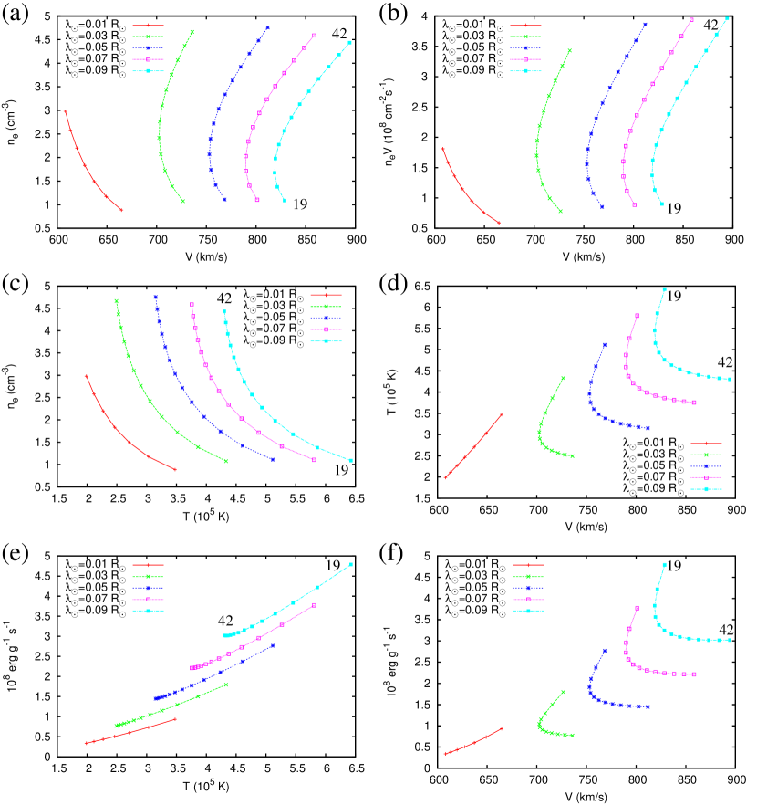
Figure 2: Values at 1 AU of wind speed, density, mass flux, temperature, and heating per unit mass for different combinations of $z_{+}^{\odot}$ (amplitude of the perturbation at the base) and $\lambda_{\odot}$ (correlation scale of the turbulence). For each curve of constant $\lambda_{\odot}$, $z_{+}^{\odot}$ is varied uniformly between 19 and 42 km/s (except the case with $\lambda_{\odot}=0.01~{}R_{\odot}$ and $\lambda_{\odot}=0.03~{}R_{\odot}$ for which no steady-solution is found at the highest values of $z_{+}^{\odot}$): (a) density vs. wind speed; (b) mass flux vs. wind speed; (c) density vs. temperature; (d) temperature vs.  wind speed; (e) heating per unit mass vs. temperature; (f) heating per unit mass vs. wind speed.

Having shown that we can reproduce a solution of Verdini et al. (2010) without thermal conduction and radiation losses, we now reintroduce them into Eq. (3) to complete a parameter space study. We also use different values of density and temperature at the base of the domain of $n_{0}=2\times 10^{12}~{}\mathrm{cm^{-3}}$ and $T_{0}=20{,}000~{}\mathrm{K}$ respectively, to include the transition region and upper chromosphere in the calculation. The use of these boundary conditions at the base of the chromosphere is described by Mok et al. (2005) and Mikić et al. (2013). The exact value of the density is not important, as long as it is large enough to form a temperature plateau at the top of the chromosphere. As shown in Lionello et al. (2009), while using smaller values is possible, there is a risk of evaporation for the chromosphere. On the other hand, using larger values will slightly increase the thickness of the plateau, without significantly affecting the properties of the corona. A technique that artificially broadens the transition region, while maintaining accuracy in the corona is likewise employed (Lionello et al., 2009). The compressional heating term $H_{c}$ of Eq. (13) is set to zero. For the same field line described in Sec. 2, we try to calculate steady-state solar wind solutions with varying values of $z_{+}^{\odot}$ and $\lambda_{\odot}$ at the base. We consider 13 different values of $z_{+}^{\odot}$ equally spaced between $19~{}\mathrm{km/s}\lesssim z_{+}^{\odot}\lesssim 42~{}\mathrm{km/s}$, the interval between each value being $\Delta z_{+}^{\odot}\simeq 1.9~{}\mathrm{km/s}$. For $\lambda_{\odot}$ we choose 5 values within $0.01~{}R_{\odot}\leq\lambda_{\odot}\leq 0.09~{}R_{\odot}$, with an interval $\Delta\lambda_{\odot}=0.02~{}R_{\odot}$.

We are not able to obtain steady-state solution for all the values selected. In fact, when $\lambda_{\odot}=0.01~{}R_{\odot}$, non-oscillatory solutions are possible only for $19~{}\mathrm{km/s}\lesssim z_{+}^{\odot}\lesssim 31~{}\mathrm{km/s}$; when $\lambda_{\odot}=0.03~{}R_{\odot}$, we do not find a steady-state solution for $z_{+}^{\odot}\simeq 42~{}\mathrm{km/s}$. In Fig. 2 we present the values at 1 AU of wind speed, density, mass flux, temperature, and heating per unit mass for the all the steady-state solutions. The different panels display how the variations of the amplitude of the boundary condition $z_{+}^{\odot}$, for each value of $\lambda_{\odot}$, changes the properties of the solution. Fig. 2a shows that an increase in $z_{+}^{\odot}$ leads to higher densities at 1 AU, with less marked changes in the wind speed. Not surprisingly, the same applies to the mass flux as a function of the wind speed (Fig. 2b). However, as it appears from Fig. 2c, for a given $\lambda_{\odot}$, changing $z_{+}^{\odot}$ has noticeable effects both on the temperature and the density of the wind at 1 AU. Figure 2d indicates that, by changing the turbulent length scale $\lambda_{\odot}$, we increase both speed and temperature of the wind at Earth. This direct proportionality of wind temperature and density is discussed in the analysis of Elliott et al. (2012), who showed how the $T-V$ relationship, except for transient phenomena, is a particularly robust one. Finally, Figs. 2e and 2f show the heating rate per unit mass as a function respectively of the temperature and the wind speed. Vasquez et al. (2007) presented solar wind measurements and showed how the turbolent heating rates (both expected and calculated) correlate with the temperature and the wind speed. Notwithstanding the differences between the models, our results appear to be roughly within the spread in values shown in Figs. 7 and 10 of Vasquez et al. (2007). If we compare our values with those obtained from in situ measurements (e.g. Sokół et al., 2013), we find that selecting a combination of $\lambda_{\odot}$ and $z_{+}^{\odot}$ such as $0.03~{}R_{\odot}\lesssim\lambda_{\odot}\lesssim 0.07~{}R_{\odot}$ and $23~{}\mathrm{km/s}\lesssim z_{+}^{\odot}\lesssim 31~{}\mathrm{km/s}$ yields solutions compatible with observations.

3.3 Example of a Fast Wind Solution

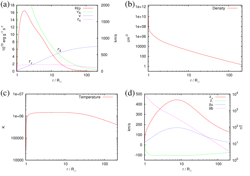
Figure 3: Fast wind solution with $z_{+}^{\odot}=25~{}\mathrm{km/s}$, $\lambda_{\odot}=0.05~{}R_{\odot}$, thermal conduction, and radiative losses. (a) Heating per unit mass (left scale), wind speed, Alfvén speed, sound speed (right scale). The bulk of the heating is deposited within the critical point for Alfvén waves (marked $r_{A}$, while the sound critical point is at $r_{s}$). (b) Number density; (e) Temperature. (d) The amplitudes of the perturbations, $z_{+}$ and $z_{-}$, of their average, $\delta u$ (left scale), and of $\delta b$ (right scale).

We now discuss in more details one of the solutions obtained in Sec. 3.2. Among the possible choices of fast solar wind solutions, we select the one with $z_{+}^{\odot}=25~{}\mathrm{km/s}$ and $\lambda_{\odot}=0.05~{}R_{\odot}$, which yields a wind speed of 753 km/s and a number density of $2.06~{}\mathrm{cm}^{-3}$ at 1 AU. In Fig. 3a, we plot wind speed, Alfvén speed, and sound speed together with the heating per unit mass. The bulk of the heating is deposited below the critical Alfvén point, where the wind is sub-Alfvénic. Figures 3c and 3d show the behavior of the density and temperature respectively. Introducing thermal conduction creates a temperature plateau between 2 and 10 $R_{\odot}$ and, consequently, also a relatively constant sound speed (Fig. 3a). In Fig. 3c we plot the two components of the perturbation, $z_{+}$ and $z_{-}$, their average, $\delta u$, and the perturbation of the magnetic field, $\delta b$. The values of $\delta u$ are compatible with observations that lie in the range $\delta u=90\pm 30~{}\mathrm{km/s}$ at $4~{}R_{\odot}$ and $\delta u=150\pm 100~{}\mathrm{km/s}$ at $10-15~{}R_{\odot}$ (Withbroe, 1988). $\delta b$ is also within the range of values as measured by Helios 1 at a distance from the Sun between 0.66 and 0.60 AU (Fig. 5-4 of Tu & Marsch, 1995) and Helios 2 at a distance from the Sun of 0.9 AU (Fig. 9 of Bruno & Carbone, 2013).

While the values of the photospheric correlation length we have used in the model are of the order of the supergranular sizes on the solar surface, there is evidence from both direct observations of the photosphere (Abramenko et al., 2013) and radio scintillations of the corona (Hollweg et al., 2010) that $\lambda_{\odot}$ may be as small as 0.0003 to 0.001 $R_{\sun}$. If, for the case here described, we reduce the correlation length to $\lambda_{\odot}=0.001~{}R_{\sun}$, this lowers the wind speed at 1 AU to 610 km/s, but also lowers the density to only $0.7~{}\textrm{cm}^{-3}$, which is far below the measurements of the slow solar wind. Therefore it appears that smaller values of $\lambda_{\odot}$ are not sufficient to reproduce the parameter space of the slow solar wind, although the effects of the different properties (e.g., larger expansion factors) of the magnetic field lines associated to the slow stream should be explored.

4 DISCUSSION

We have implemented a time-dependent model of the solar wind with acceleration and heating through turbulence dissipation. Our model uses the self-consistent formulation of Verdini et al. (2010) within a 1D HD code with thermal conduction and radiation losses. For the case of a simplified energy equation, such as that used by Verdini et al. (2010), we accurately reproduce a solar wind solution. When the model is extended by introducing thermal conduction and radiative losses, our model produces fast solar wind solutions whose characteristics are compatible with in situ measurements. The model of Verdini et al. (2010) includes a compressional heating in the lower corona; we have found that it is not necessary to include such phenomenological heating when a more realistic energy equation is used. Our model, in comparison with that of Lionello et al. (2013), is certainly more complicated, since it advances the amplitude of the perturbations rather than the energies as the latter does. Moreover, the model of Lionello et al. (2013) neglects the contribution of the Reynolds stress, assuming that outwardly propagating wave is dominant. However, with the present method, we have found that the contribution of the Reynolds stress can be sizable; in one particular case it lowered the wind speed by approximately $25\%$.

Furthermore, if we consider the integration of turbulence dissipation heating and acceleration in 3D MHD models, there are several advantages in the present formulation in respect of that of Lionello et al. (2013). First, it is not much more computationally demanding to advance the amplitudes rather the energies. Second, this formulation in terms of $z_{\pm}$ does not require us to calculate for each mesh point the reflection coefficient along each field line passing through it. Third, in our experience the inclusion of time-dependent transport equations for $z_{\pm}$ does not increase the physical convergence time to steady state. Finally, as shown by Usmanov et al. (2011), the Reynolds stress term can be written for a case when only perturbations perpendicular to the large scale magnetic field are considered and whose actual directions do not play a significant role. Therefore we believe that the present formulation can be readily extended to the 3D model of Lionello et al. (2009).

References

- Abramenko et al. (2013) Abramenko, V. I., Zank, G. P., Dosch, A., Yurchyshyn, V. B., Goode, P. R., Ahn, K., & Cao, W. 2013, ApJ, 773, 167
- Athay (1986) Athay, R. G. 1986, ApJ, 308, 975
- Belcher & Davis (1971) Belcher, J. W., & Davis, Jr., L. 1971, J. Geophys. Res., 76, 3534
- Breech et al. (2008) Breech, B., Matthaeus, W. H., Minnie, J., Bieber, J. W., Oughton, S., Smith, C. W., & Isenberg, P. A. 2008, Journal of Geophysical Research (Space Physics), 113, 8105
- Bruno & Carbone (2013) Bruno, R., & Carbone, V. 2013, Living Reviews in Solar Physics, 10, 2
- Chandran et al. (2011) Chandran, B. D. G., Dennis, T. J., Quataert, E., & Bale, S. D. 2011, ApJ, 743, 197
- Coleman (1968) Coleman, Jr., P. J. 1968, ApJ, 153, 371
- Cranmer (2010) Cranmer, S. R. 2010, ApJ, 710, 676
- Cranmer & van Ballegooijen (2005) Cranmer, S. R., & van Ballegooijen, A. A. 2005, ApJS, 156, 265
- Cranmer et al. (2007) Cranmer, S. R., van Ballegooijen, A. A., & Edgar, R. J. 2007, ApJS, 171, 520
- de Karman & Howarth (1938) de Karman, T., & Howarth, L. 1938, Royal Society of London Proceedings Series A, 164, 192
- Dmitruk et al. (2001) Dmitruk, P., Milano, L. J., & Matthaeus, W. H. 2001, ApJ, 548, 482
- Dobrowolny et al. (1980) Dobrowolny, M., Mangeney, A., & Veltri, P. 1980, Physical Review Letters, 45, 144
- Elliott et al. (2012) Elliott, H. A., Henney, C. J., McComas, D. J., Smith, C. W., & Vasquez, B. J. 2012, Journal of Geophysical Research (Space Physics), 117, 9102
- Goedbloed et al. (2010) Goedbloed, J. P., Keppens, R., & Poedts, S. 2010, Advanced Magnetohydrodynamics (Cambridge, UK: Cambridge University Press)
- Grappin et al. (1983) Grappin, R., Leorat, J., & Pouquet, A. 1983, A&A, 126, 51
- Habbal et al. (1995) Habbal, S. R., Esser, R., Guhathakurta, M., & Fisher, R. R. 1995, Geophys. Res. Lett., 22, 1465
- Hammer (1982a) Hammer, R. 1982a, ApJ, 259, 779
- Hammer (1982b) —. 1982b, ApJ, 259, 767
- Hansteen & Leer (1995) Hansteen, V. H., & Leer, E. 1995, J. Geophys. Res., 100, 21577
- Hansteen et al. (1997) Hansteen, V. H., Leer, E., & Holzer, T. E. 1997, ApJ, 482, 498
- Heinemann & Olbert (1980) Heinemann, M., & Olbert, S. 1980, J. Geophys. Res., 85, 1311
- Hollweg (1976) Hollweg, J. V. 1976, J. Geophys. Res., 81, 1649
- Hollweg (1978) —. 1978, Reviews of Geophysics and Space Physics, 16, 689
- Hollweg (1986) —. 1986, J. Geophys. Res., 91, 4111
- Hollweg et al. (2010) Hollweg, J. V., Cranmer, S. R., & Chandran, B. D. G. 2010, ApJ, 722, 1495
- Hollweg & Johnson (1988) Hollweg, J. V., & Johnson, W. 1988, J. Geophys. Res., 93, 9547
- Holzer & Leer (1980) Holzer, T. E., & Leer, E. 1980, J. Geophys. Res., 85, 4665
- Hossain et al. (1995) Hossain, M., Gray, P. C., Pontius, Jr., D. H., Matthaeus, W. H., & Oughton, S. 1995, Physics of Fluids, 7, 2886
- Kopp & Holzer (1976) Kopp, R. A., & Holzer, T. E. 1976, Sol. Phys., 49, 43
- Lionello et al. (2009) Lionello, R., Linker, J. A., & Mikić, Z. 2009, ApJ, 690, 902
- Lionello et al. (1999) Lionello, R., Mikić, Z., & Linker, J. A. 1999, Journal of Computational Physics, 152, 346
- Lionello et al. (1998) Lionello, R., Mikić, Z., & Schnack, D. D. 1998, Journal of Computational Physics, 140, 1
- Lionello et al. (2013) Lionello, R., Velli, M., Linker, J. A., & Mikić, Z. 2013, in American Institute of Physics Conference Series, Vol. 1539, American Institute of Physics Conference Series, ed. G. P. Zank, J. Borovsky, R. Bruno, J. Cirtain, S. Cranmer, H. Elliott, J. Giacalone, W. Gonzalez, G. Li, E. Marsch, E. Moebius, N. Pogorelov, J. Spann, & O. Verkhoglyadova, 30–33
- Matthaeus et al. (2004) Matthaeus, W. H., Minnie, J., Breech, B., Parhi, S., Bieber, J. W., & Oughton, S. 2004, Geophys. Res. Lett., 31, 12803
- Matthaeus et al. (1999) Matthaeus, W. H., Zank, G. P., Oughton, S., Mullan, D. J., & Dmitruk, P. 1999, ApJ, 523, L93
- Mikić et al. (1999) Mikić, Z., Linker, J. A., Schnack, D. D., Lionello, R., & Tarditi, A. 1999, Phys. of Plasmas, 6, 2217
- Mikić et al. (2013) Mikić, Z., Lionello, R., Mok, Y., Linker, J. A., & Winebarger, A. R. 2013, ApJ, 773, 94
- Mok et al. (2005) Mok, Y., Mikić, Z., Lionello, R., & Linker, J. A. 2005, ApJ, 621, 1098
- Sokół et al. (2013) Sokół, J. M., Bzowski, M., Tokumaru, M., Fujiki, K., & McComas, D. J. 2013, Sol. Phys., 285, 167
- Sokolov et al. (2013) Sokolov, I. V., van der Holst, B., Oran, R., Downs, C., Roussev, I. I., Jin, M., Manchester, IV, W. B., Evans, R. M., & Gombosi, T. I. 2013, ApJ, 764, 23
- Suzuki & Inutsuka (2005) Suzuki, T. K., & Inutsuka, S.-i. 2005, ApJ, 632, L49
- Tu & Marsch (1995) Tu, C.-Y., & Marsch, E. 1995, Space Sci. Rev., 73, 1
- Usmanov et al. (2012) Usmanov, A. V., Goldstein, M. L., & Matthaeus, W. H. 2012, ApJ, 754, 40
- Usmanov et al. (2011) Usmanov, A. V., Matthaeus, W. H., Breech, B. A., & Goldstein, M. L. 2011, ApJ, 727, 84
- van der Holst et al. (2010) van der Holst, B., Manchester, W. B., Frazin, R. A., Vásquez, A. M., Tóth, G., & Gombosi, T. I. 2010, ApJ, 725, 1373
- van der Holst et al. (2013) van der Holst, B., Sokolov, I. V., Meng, X., Jin, M., Manchester, IV, W. B., Toth, G., & Gombosi, T. I. 2013, ArXiv e-prints
- Vasquez et al. (2007) Vasquez, B. J., Smith, C. W., Hamilton, K., MacBride, B. T., & Leamon, R. J. 2007, Journal of Geophysical Research (Space Physics), 112, 7101
- Velli (1993) Velli, M. 1993, A&A, 270, 304
- Velli (1994) —. 1994, Advances in Space Research, 14, 123
- Verdini & Velli (2007) Verdini, A., & Velli, M. 2007, ApJ, 662, 669
- Verdini et al. (2010) Verdini, A., Velli, M., Matthaeus, W. H., Oughton, S., & Dmitruk, P. 2010, ApJ, 708, L116
- Withbroe (1988) Withbroe, G. L. 1988, ApJ, 325, 442
- Withbroe & Noyes (1977) Withbroe, G. L., & Noyes, R. W. 1977, ARA&A, 15, 363
- Zank et al. (2012) Zank, G. P., Dosch, A., Hunana, P., Florinski, V., Matthaeus, W. H., & Webb, G. M. 2012, ApJ, 745, 35