A Model for the Sources of the Slow Solar Wind
Abstract
Models for the origin of the slow solar wind must account for two seemingly-contradictory observations: The slow wind has the composition of the closed-field corona, implying that it originates from the continuous opening and closing of flux at the boundary between open and closed field. On the other hand, the slow wind also has large angular width, up to , suggesting that its source extends far from the open-closed boundary. We propose a model that can explain both observations. The key idea is that the source of the slow wind at the Sun is a network of narrow (possibly singular) open-field corridors that map to a web of separatrices and quasi-separatrix layers in the heliosphere. We compute analytically the topology of an open-field corridor and show that it produces a quasi-separatrix layer in the heliosphere that extends to angles far from the heliospheric current sheet. We then use an MHD code and MDI/SOHO observations of the photospheric magnetic field to calculate numerically, with high spatial resolution, the quasi-steady solar wind and magnetic field for a time period preceding the August 1, 2008 total solar eclipse. Our numerical results imply that, at least for this time period, a web of separatrices (which we term an S-web) forms with sufficient density and extent in the heliosphere to account for the observed properties of the slow wind. We discuss the implications of our S-web model for the structure and dynamics of the corona and heliosphere, and propose further tests of the model.
1 Introduction
Decades of in situ measurements of the heliosphere have firmly established that the Sun’s wind consists of two distinct types: “fast” and “slow”. In terms of its origins at the Sun, the best understood is the fast wind, which typically exhibits speeds in excess of 600 km/s at 1 AU and beyond (e.g., McComas et al., 2008). The fast wind is measured to be approximately steady, except for some Alfvénic turbulence (e.g., Bame et al., 1977; Bruno & Carbone, 2005). This wind is known to originate from coronal holes, regions that appear dark in XUV and X-ray images, due to a plasma density that is substantially lower () than in surrounding coronal regions (Zirker, 1977). As implied by eclipse and coronagraph images, the magnetic field in coronal holes is open—appearing mainly radial and stretching out without end—whereas the field in the surrounding regions is closed, looping back down to the photosphere. Hence, the fast wind corresponds to the steady wind predicted by Parker in his classic work (Parker, 1958, 1963).
The slow wind, however, is much less understood. In particular, its origin at the Sun has long been one of the major unsolved problems in solar/heliospheric physics. This wind has a number of observed features that distinguish it physically from the fast wind. First, its speeds are typically slower, . More important, the slow wind appears to be inherently non-steady when compared to the fast wind (e.g., Bame et al., 1977; Schwenn, 1990; Gosling, 1997; McComas et al., 2000). It exhibits strong and continuous variability in both plasma (for example, speed and composition) and magnetic field properties; variability that cannot be described as simply Alfvénic disturbances superimposed on a steady background (Zurbuchen & von Steiger, 2006; Bruno & Carbone, 2005). Finally, its location in the heliosphere is distinct; it is generally found surrounding the heliospheric current sheet (HCS) (e.g., Burlaga et al., 2002). A key point is that the HCS is always embedded inside slow wind, never fast. From the presently available spacecraft observations, it is not possible to rule out the possibility that slow wind also occurs in locations unconnected to the HCS, in other words, that there are pockets of slow wind with no embedded HCS and surrounded completely by fast wind. However, the present data are certainly consistent with the picture that, at least, during solar minimum when the corona-wind mapping can be determined with some accuracy, all slow wind originates from a band that encompasses the HCS, so that the mapping of the slow wind down to the Sun appears to connect to or near the helmet streamer belt (e.g., Gosling, 1997; Zhao et al., 2009).
Another key feature of the slow wind is its latitudinal extent, which typically ranges from – near solar minimum, a time when it is easiest to distinguish the sources of fast and slow wind. Within this broad region of slow wind the actual HCS, across which the magnetic field changes direction, is very narrow. As for any current sheet, one can identify in the heliospheric data a scale over which the field becomes small and the plasma beta, defined as the ratio of the gas pressure to the magnetic pressure , becomes large. This region is termed the plasma sheet and is usually of the order of a few degrees in angular width (e.g., Winterhalter et al., 1994; Bavassano et al., 1997; Wang et al., 2000; Crooker et al., 2004). It is important to note that the HCS is often not symmetrically located within the broad band of slow wind, but is often found nearer to one edge of the slow wind region (Burlaga et al., 2002). It is also important to note that the field almost never vanishes at the HCS, as would be expected for a true steady-state. This observation implies that, at least, the wind near the HCS must be continuously dynamic.
The final and most critical feature of the slow wind that distinguishes it from the fast is the plasma composition (Geiss et al., 1995; von Steiger et al., 1995). It is well-known that in the closed field corona, the ratio of the abundances of elements with low first ionization potential (FIP), such as Mg and Fe, to those with high FIP, such as C and Ne, is a factor 4 or so higher than in the photosphere (e.g., Meyer, 1985; Feldman & Widing, 2003). This so-called FIP effect is not seen in the fast wind, which has abundances similar to those of the photosphere; but, it is present in the slow wind, which has abundances similar to that of the closed corona (Gosling, 1997; Zurbuchen & von Steiger, 2006; Zurbuchen, 2007).
Along with the difference in elemental abundances, the slow and fast wind also exhibit clear differences in their ion charge state abundances, for example, the ratio of . This ratio can be used to determine the “freeze-in” temperature of the ion charge states at the source of the wind. Close to the Sun where the time scales for ionization and recombination are much shorter than the plasma’s expansion time-scales, the ion charge states are approximately in ionization equilibrium with the local electron temperature. As the solar wind plasma expands outward, however, the electron density drops rapidly and the recombination time scales become so large that the ionic charge states stop changing, freezing-in the electron temperature at this point. The freeze-in radius varies for the different ions, but is typically 1 - 3 R⊙. The data show that the slow wind has a higher freeze-in temperature () than the fast wind () (von Steiger et al., 1997, 2001; Zurbuchen et al., 1999, 2002). Note, however, that this freeze-in temperature corresponds only to the electron temperature in the low corona. The proton and ion temperatures measured in situ and in coronal holes by UVCS, for example, (e.g., Kohl et al., 2006) show the opposite trend in that the ion temperatures are substantially higher in the fast wind than in the slow (Marsch, 2006). The origin of these differences in the ion temperatures between the two winds is still not clear, but in any case, both the ion and freeze-in temperatures suggest that the sources of the two winds near the Sun are physically different.
The elemental abundances track very well the ionic abundances, indicating that there is a consistent compositional distinction between the two winds. Furthermore, the two winds have markedly different temporal variability in elemental and ionic composition. The fast exhibits an approximately constant composition; whereas the slow exhibits large and continuous variability, so that its elemental composition varies from coronal to near photospheric. The composition results suggest that the fast wind has a unique origin, presumably in coronal holes, but that the slow wind originates from a mixture of sources.
In fact, Zurbuchen and coworkers have argued that the compositional differences, rather than the speed, are what truly distinguish the two winds, because it is possible to find solar wind whose composition and constancy match that of the “fast wind,” but that has relatively slow speed, (Zhao et al., 2009). Note also that, as determined by the composition measurements (Zurbuchen et al., 1999), the boundary between the slow and fast wind in the heliosphere is sharp, of order a few degrees in angular extent, much smaller than the angular width of the slow wind region, but comparable to that of the plasma sheet. An important point is that the observed sharpness of the composition transition is not merely a dynamical effect, because it does not depend on whether the stream-stream transition is fast to slow or slow to fast (Geiss et al., 1995; Zurbuchen, 2007). We conclude, therefore, that the fast and slow winds are far more appropriately described as the steady and unsteady winds, and that the boundary layer between the two winds is much narrower than the width of either wind.
Since the differences in plasma composition of the two winds must be due to differences in their origins at the Sun, the composition data place severe constraints on the possible sources of the slow wind. In particular, the data imply that the slow wind originates in the dynamic opening of closed magnetic flux, which releases closed-corona plasma into the wind. Such a process would also naturally explain the difference in variability between the fast and slow wind.
It should be emphasized, however, that this constraint on the slow wind’s origin is not universally accepted. Several authors have argued that the slow wind originates from open-field coronal holes, just like the fast wind, but from the edges of the holes, where the field expands super-radially as it extends from the photosphere out to the heliosphere (e.g., Kovalenko, 1981; Wang & Sheeley, 1991; Cranmer & van Ballegooijen, 2005; Cranmer et al., 2007; Wang et al., 2009). The hypothesis is that a large expansion factor can both slow down the wind by affecting the location of wave energy deposition in coronal flux tubes, and change the plasma composition by the FIP mechanism proposed by Laming (2004). Note that in the expansion factor model, as in all steady state wind solutions, the properties of the wind in a given flux tube are determined uniquely, in most cases, by the flux tube geometry and the forms of the heating and momentum deposition (Cranmer et al., 2007). Of course the detailed forms of the heating and momentum deposition will depend on the flux tube geometry, and may depend on other factors, as well, but the dependence on these other factors cannot be dominant; otherwise the calculated wind speed would not be well correlated with expansion factor. In other words, two flux tubes on the Sun with identical geometry should have similar heating/momentum deposition and end up with the same wind properties. Therefore, the steady-state models inherently predict a tight correlation between speed and composition (e.g., Cranmer et al., 2007).
The problem, however, is that observations indicate that wind speed is not tightly correlated with composition. The wind from small equatorial coronal holes with a large expansion factor is indeed slow, with speeds , in good agreement with the predictions of the expansion factor models. But this wind has photospheric FIP ratios, so it is still considered to be “fast wind” (Zhao et al., 2009). Furthermore, this not-so-fast wind has the temporal quasi-steadiness of the fast wind, rather than the quasi-chaotic time variation of the slow wind.
We conclude, therefore, that the most likely source for the true slow wind, that with FIP-enhanced coronal composition, is the closed-field corona. In this case, the process that releases the coronal plasma to the wind must be either the opening of closed flux or interchange reconnection between open and closed magnetic field lines. This latter process is the underlying mechanism invoked by Fisk and co-workers (Fisk et al., 1998; Fisk, 2003; Fisk & Zhao, 2009) in their model for the heliospheric field. These authors argue that open flux can diffuse freely throughout the solar surface, even deep inside the helmet streamer region. If so, then the interchange reconnection between open and closed magnetic field lines would naturally account for both the composition and geometrical properties of the slow wind. The difficulty with this model is that it has not been demonstrated that such open flux diffusion can actually occur. In fact, detailed MHD simulations indicate that it is difficult to bring open fields into closed-field regions without having them close down (Edmondson et al., 2010; Linker et al., 2010). The simulation results are in agreement with Antiochos et al. (2007), who argued that, for the low-beta corona, basic MHD force balance forbids the presence of open flux deep inside the closed helmet streamer region.
Within the context of MHD models, the most likely location for the release of closed-field plasma is from the tops of helmet streamers (the Y-point at the bottom of the HCS), where the balance between gas pressure and magnetic pressure is most sensitive to perturbations. A number of authors have argued that streamer tops are unstable and should undergo continual opening and closing as a result of thermal instability (Suess et al., 1996; Endeve et al., 2004; Rappazzo et al., 2005). Even if streamer tops are stable, it seems inevitable that the constant emergence and disappearance of photospheric flux and the constant motions of the photospheric would force them to be continuously evolving. Furthermore, coronagraph observations often show the ejection of “blobs” from the tops of streamers and into the HCS (Sheeley et al., 1997).
Although this streamer top model seems promising in that it naturally explains both the composition and variability, it has difficulty in accounting for the large angular widths of the slow wind. One would expect the instabilities to be confined to the high-plasma beta region about the current sheet. In fact, the plasma emanating from the streamer tops, the so-called stalks, is observed to be only – wide, which agrees well with the plasma sheet width in the heliosphere (Bavassano et al., 1997; Wang et al., 2000). Even if the plasma sheet width were to be widened by the Kelvin-Helmholtz instability (e.g., Einaudi et al., 1999), there would not be enough mass flux from the narrow region at the streamer tops to account for the slow wind. The streamer-top models can account for a thin band of slow wind around the HCS, but it seems unlikely that this is the origin of the bulk of the slow wind, which can extend as far as in latitude from the HCS.
In order to be compatible with the in situ data, we require some process that releases closed-field plasma onto open field lines that, in the heliosphere, can be far from the HCS. This requirement seems impossible to satisfy, because the plasma release must occur at the boundary between the open and closed field in the corona, which maps directly to the HCS. We describe below, however, a magnetic topology that resolves this slow wind paradox: the flux associated with an open-field corridor can be simultaneously near to and far from the open-closed boundary!
2 The Topology of an Open-Field Corridor
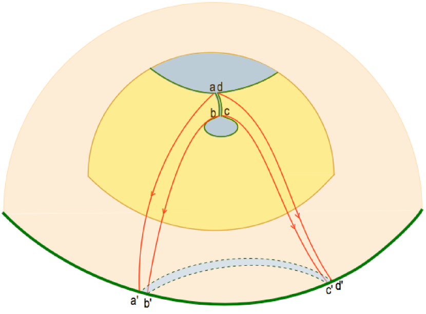
Figure 1 illustrates the magnetic connectivity from the photosphere to the heliosphere that results from an open-field corridor. The dark yellow inner sphere in the figure represents the photosphere, while the light yellow, semi-transparent one represents an arbitrary radial surface in the open-field heliosphere, say at The green line on the photosphere marks the boundary between open (gray) and closed (yellow) field regions, which is mapped by the magnetic field (red lines) to the HCS (thick green line) at the surface. The green line at the HCS is also the polarity inversion line at this surface. Note that the four points, a, b, c, and d, which are meant to represent the end-points of the corridor at the Sun, map sequentially to the corresponding points a′, b′, c′, and d′ along the HCS.
The open field pattern at the photosphere of Fig. 1 consists of a large polar coronal hole and, as is often seen, a smaller low-latitude hole. In recent work, we argued that if the two holes are in the same photospheric polarity region, then by our uniqueness conjecture the holes must be connected by an open field corridor, as illustrated above (Antiochos et al., 2007). It is evident from the figure that the flux in the corridor maps on the heliospheric surface to a thin arc (light gray band), bounded at both ends by the HCS. The flux between the arc and the HCS maps to the low-latitude extension while the flux outside the arc maps to the main part of the polar coronal hole. The corridor and its associated arc are the footprints of two quasi-separatrix layers (QSLs, e.g., Priest & Démoulin, 1995; Démoulin et al., 1996) that combine into a hyperbolic flux tube, as has been described in detail by Titov et al. (2002, 2008) for the case of closed magnetic configurations. In contrast, the HCS is a true separatrix.
The key point for understanding the origin of the slow wind is that, just like the HCS, the QSL arc in the heliosphere can also be a source region for slow wind. If the open-field corridor at the Sun is sufficiently narrow, then the continual evolution of the photosphere, driven by the ever-present supergranular flow and flux emergence/submergence in particular, will continually change the exact location of this corridor. But, by the uniqueness conjecture (Antiochos et al., 2007), the corridor is a topologically robust feature, similar to a null-point, and must be present on the photosphere as long as the low-latitude coronal hole extension is present. Its location and shape, however, will vary in response to local photospheric changes. These variations require field line opening/closing and interchange reconnection, thereby releasing closed-field plasma all along the QSL arc in the heliosphere. Therefore, if the QSL arc extends to high latitudes, this will naturally produce slow wind with an extent far from the HCS.
To determine whether the QSL resulting from an open field corridor does, indeed, reach high heliospheric latitudes, we have calculated an example of a field such as that of Fig. 1 using the source surface model (Altschuler & Newkirk, 1969; Schatten et al., 1969; Hoeksema, 1991). The field is most easily determined from the image-dipole formula derived by Antiochos et al. (2007). For a dipole with moment located at a point inside the Sun, and a source surface at radius , the magnetic field is determined from the potential via , where is given by:
| (1) |
This field satisfies the source-surface boundary condition that at , since there. The advantage of this formulation is that most active regions can be approximated by a collection of dipoles, and one can build up a field of arbitrary complexity by simply adding a series of dipoles of the form of Eq. (1). Each dipole is specified in terms of its position in spherical coordinates , where , , and specify the location of the dipole, and the spherical components of its dipole moment, .
Figure 2 shows the field computed from Eq. (1) for the case of two dipoles: a sun-centered global dipole with a dipole moment of unit magnitude directed along the north polar axis, and an equatorial “active region” dipole at with a northward-pointing dipole moment . The source surface radius is chosen as , though the exact value is not critical for our argument. Note that for convenience in viewing the magnetic field, we have selected the dipole parameters so that the system has symmetry across both the equatorial and meridional planes. Also, for ease of viewing, we show in the Fig. 2 only the front hemisphere defined by the angular region and .
The solar surface, the photosphere, corresponds to the gray grid in Fig. 2. The colored contours on this surface correspond to contours of radial flux, indicating the presence of the active region dipole at the equator. We selected the parameters for the active region dipole so that its structure would be easily resolved. It is evident from Fig. 2 that the region is large compared to real active regions, which are generally only a few degrees in angular extent. On the other hand, the maximum field strength at the dipole center is only times that of the polar region, which is much less than the corresponding ratio for solar active regions, so the flux ratio between the active region and global background field is approximately correct. This ratio is the important parameter to obtain a coronal hole extension.
The thick black line along the equator is the contour, i.e., the polarity inversion line. The thick black line above the solar surface is the polarity inversion line at the source surface, i.e., the bottom of the HCS. Red field lines are traced at equal intervals along the HCS down to the solar surface. These define the boundary between open and closed field lines. As expected, the effect of the equatorial dipole is to pull the open-closed boundary down to lower latitudes; in other words, to create a low-latitude extension of the coronal hole, which can be seen as the gray shaded region in the Figure. Far from the dipole, the coronal hole boundary is at a latitude of , whereas at the meridional symmetry plane the boundary drops down to .
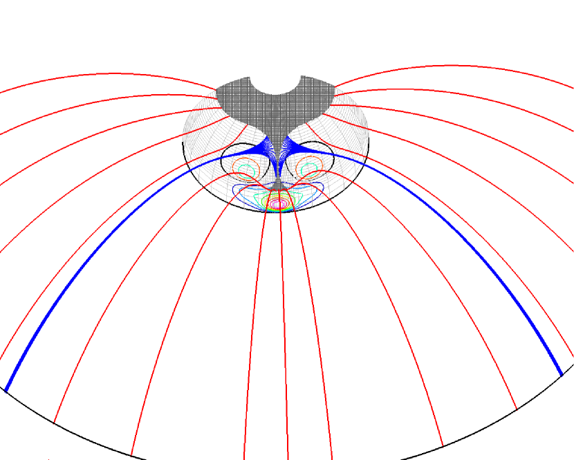
For the large spatial scale of our active region dipole, the extension of the coronal hole down to low latitudes is gradual rather than in the form of a distinct “elephant trunk”, but the basic effect is clearly present. There is no open-field corridor in Fig. 2, but let us now add another dipole to the system, displaced in both latitude and longitude from the equatorial one and a factor of five times weaker. This dipole is located at with a primarily southward-pointing dipole moment . In order to maintain the equatorial and meridional symmetry, as mentioned earlier, we actually add 4 dipoles symmetrically located about the equatorial and meridional planes.
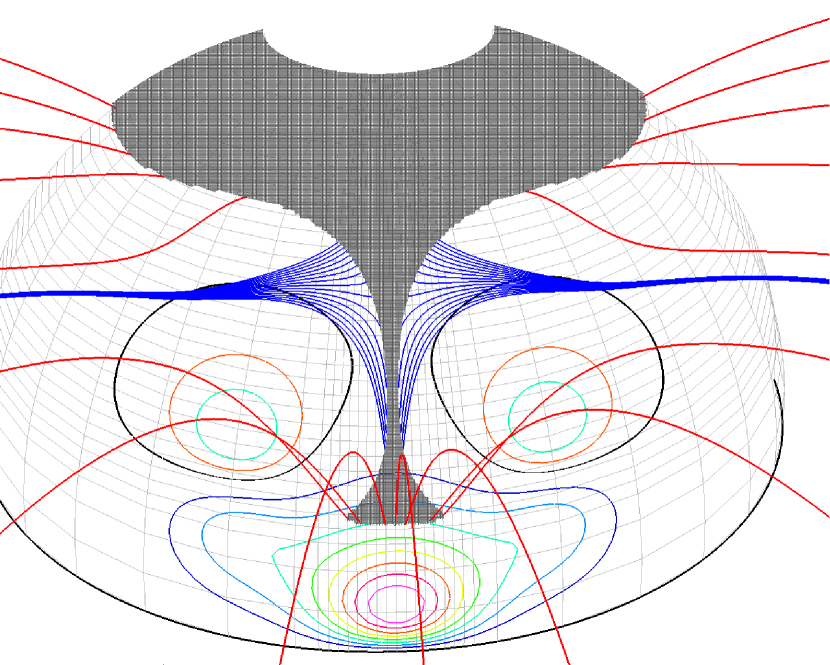
The resulting field is shown in Figure 3. The effect of the additional dipoles is to add high-latitude polarity inversion lines to the system. These “squeeze” the open-flux extension of Fig. 2 to form a narrow corridor and a low-latitude coronal hole. As in Fig. 2, red field lines are traced from equidistant footpoints along the HCS down to the solar surface. The red footpoints at the photosphere appear to traverse the boundary of the low-latitude hole and then jump abruptly to the polar hole boundary, which implies that the mapping defined by the field develops extreme gradients in the region connecting the two holes. To clarify this point, we have traced two sets of field lines, colored in blue, from footpoints that are closely located at the HCS. The corresponding solar footpoints are much more widely spaced, running along the corridor. The resulting structure, Fig. 3, looks very similar to the mapping drawn in Fig. 1, in that the closely spaced pairs of points a′,b′ and c′,d′ at the HCS map to far-separated points a,b and c,d at the solar surface. Note also that although the footpoints of the two sets of blue lines approach each other very closely at the photosphere, they are far separated at the HCS, by a distance of order . This result indicates that even though the low-latitude coronal hole has small area, it contains a substantial magnetic flux. As is evident from the colored contours in Fig. 3, the photospheric field strength in the low-latitude hole is large due to the presence of the active region dipole.
The analytic model underlying Fig. 3 has similar topology to the case shown schematically in Fig. 1. The low-latitude coronal hole extension in Fig. 3 is connected to the main polar hole by a corridor that becomes very narrow. Furthermore, this type of topology is not difficult to obtain. It is often observed in quasi-steady MHD solutions for observed photospheric fields, as will be shown below. A similar corridor was found for Carrington rotation 1922 (Antiochos et al., 2007).
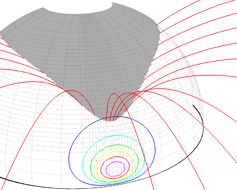
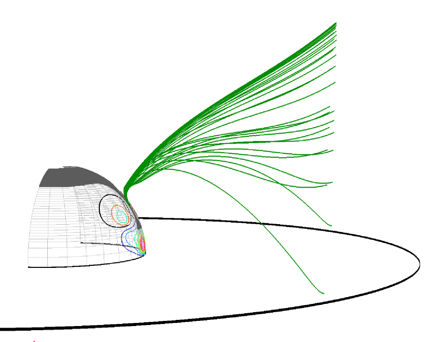
The question now is whether the open flux in the corridor connects to large latitudes in the heliosphere. To answer this question, we trace field lines from a set of photospheric footpoints lying on a latitudinal line segment spanning the narrowest width of the corridor, which is only of order at the photosphere. Fig. 4b shows the footpoints and the field lines (green) near the photosphere and Fig. 4a shows where they map to on the source surface. We note that the corridor maps to high latitudes. In fact, for this analytic case, the corridor mapping defines a QSL arc that reaches latitudes , greater than that of the observed slow wind.
This result, that the corridor maps to heliospheric latitudes far above the HCS, is robust in that it is not sensitive to the exact position of the secondary dipole. The position and geometry of the corridor, on the other hand, is very sensitive to the photospheric flux distribution. For example, its width would change or even become singular (Titov et al., 2011), and its location would change substantially if the secondary dipoles were moved in longitude. Based on flux conservation arguments, and the fact that the heliospheric magnetic field is almost uniform in latitude, we can argue that the angular extent of the QSL arc, however, would be expected to depend primarily on the ratio of the flux in the low-latitude coronal hole extension to that in the polar hole. For example, in the extreme case that the fluxes were equal, the corridor mapping would be expected to reach the heliospheric pole ( from the HCS!), irrespective of the geometry of the corridor or of the coronal holes.
3 The S-Web Model
If the width of the corridor at the photosphere is small compared to the scale of typical motions there, such as the supergranular flow, we expect that the whole corridor will continuously disrupt and reform at the photosphere and, consequently, closed-field plasma will be released by reconnection all along the QSL arc in the heliosphere. Therefore, the topology of Fig. 2 may be able to resolve the slow wind paradox. The overriding question, however, is whether there are enough such corridors and corresponding QSL arcs in the heliosphere to account for the slow wind that is observed. The flux distribution of Fig. 2 produces only one such arc, which would certainly not be sufficient to reproduce the observed slow wind. There are two issues that must be addressed, the number of arcs (their density and extent on the Sun and heliosphere), and the amount of mass and energy that each arc can be expected to release. In this paper we concentrate on the first issue and only briefly discuss the second in Section 4 below, because addressing this issue requires fully dynamic calculations.
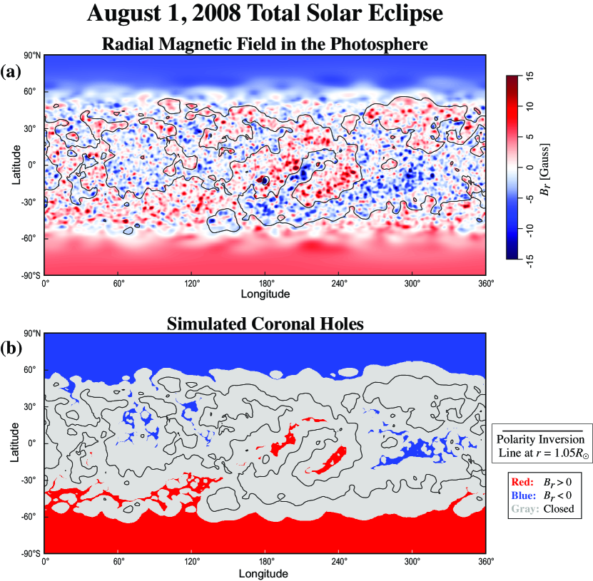
In order to address the issue of the number of QSL arcs, we calculated the quasi-steady model for an observed photospheric flux distribution. Figure 5a shows the photospheric radial field as derived from MDI observations on SOHO (Scherrer et al., 1995) for a time period preceding the August 1, 2008 total solar eclipse. This calculation was used to predict the structure of the corona prior to the eclipse, using magnetic field data measured during the period June 25–July 21, 2008. The prediction compares very favorably with images of the corona taken during the eclipse in Mongolia (Rušin et al., 2010). Note that the high resolution of the calculation captures the details of many small-scale bipoles in the photospheric magnetic field (Harvey, 1985). This has been incorporated into the idea of the “magnetic carpet” (Schrijver et al., 1997). We also show the polarity inversion line slightly above the photosphere, at to delineate the magnetic polarity of the large-scale structures. (The polarity inversion line in the photosphere itself shows an enormous complexity that overshadows its usefulness to discern the large-scale magnetic polarity.)
The quasi-steady model was calculated by using the 3D MHD code MAS. The MAS code and its implementation are described in detail by Mikić & Linker (1994), Mikić et al. (1999), Linker et al. (1999), and Lionello et al. (2009). MAS solves the time-dependent MHD equations, including a realistic energy equation with optically thin radiation and thermal conduction parallel to the magnetic field. Given the magnetic field at the photosphere and an assumption for the coronal heating source, the MHD equations are advanced until the magnetic field settles down close to steady state. MHD models are generally considered to be the most sophisticated implementation of Parker’s solar wind theory because they incorporate all the essential physics, including the balance between gas pressure and Lorentz force. An important assumption is the form of coronal heating, which is prescribed empirically at the present time since the coronal heating process is still unknown. The parameters of the empirical heating model are constrained by observations of coronal emission in EUV and X-rays (e.g., Lionello et al., 2009), as well as by solar wind measurements. Details on the assumed form for the heating and on the thermodynamics used in the MAS code can be found in Mikić et al. (2007) and Lionello et al. (2009).
In order to capture as much of the photospheric magnetic structure as possible, we ran the MAS code with unprecedented resolution. Our calculation used more than 16 million mesh cells and was run on over 4000 processors of NSF’s Ranger supercomputer at the Texas Advanced Computing Center, making it possible to include much of the small-scale structure of the photospheric field in both the quiet sun and in coronal holes, as shown in Fig. 5a. These calculations are unique in the degree to which they capture the small-scale structure of the measured magnetic field.
Figure 5b shows the distribution of open and closed magnetic field regions at the solar surface as determined by the model. It is evident that there are many low-latitude coronal hole extensions, similar to that in Fig. 3, but with much more structure. Several of these extensions appear to be disconnected from the main polar holes, but this is partly due to the limited resolution of the figure. A few of these coronal hole extensions are indeed connected by very thin corridors in the photosphere, though many are only linked to the polar coronal holes in a singular manner, as described in detail by Titov et al. (2011), and as discussed further below.
The open field pattern in Fig. 5b is clearly complex, but the important issue is the degree of complexity of the mapping into the heliosphere and, in particular, the structure of the separatrices and QSLs there. We determined the open field mapping in great detail by tracing tens of millions of magnetic field lines. The topology of this mapping, as evidenced by structures such as separatrices and QSLs, is most easily seen by analyzing the squashing factor (Titov et al., 2002; Titov, 2007). is a measure of the distortion in the magnetic field mapping, and is directly related to the gradients in the connectivity. QSLs are regions of very large ; we generally define them as any region with . True separatrices such as the HCS have infinite , because the mapping is singular there, but when computed numerically they appear as surfaces with very large (unresolved) values of . The gray arc at in Fig. 1 is a QSL in the open field, and consequently would be a region of high . The green HCS would also be a region of high (infinite) . As will be seen below, a high-resolution analysis of the properties of our MHD simulation is extremely informative.
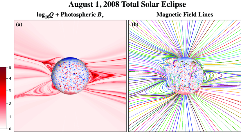
Figure 6a shows in a meridional plane at a central Carrington longitude of at the time of the eclipse at 10:21UT, while Figure 6b shows magnetic field lines traced from the vicinity of the solar limbs at the same time. We see that outlines the boundary between open and closed field, which is a true separatrix surface, but it is apparent that there is much more detailed structure in both the closed and open field regions. The complex structure of in the closed-field region is expected; it simply reflects the fact that the photospheric field consists of many small bipoles; but, there is also substantial structure in the open field near the open-closed boundary. Note the presence of a “pseudostreamer” on the NE limb, a feature that has been discussed by Wang et al. (2007). The relationship of pseudostreamers to open hole corridors and the S-web is discussed in detail in Titov et al. (2011)
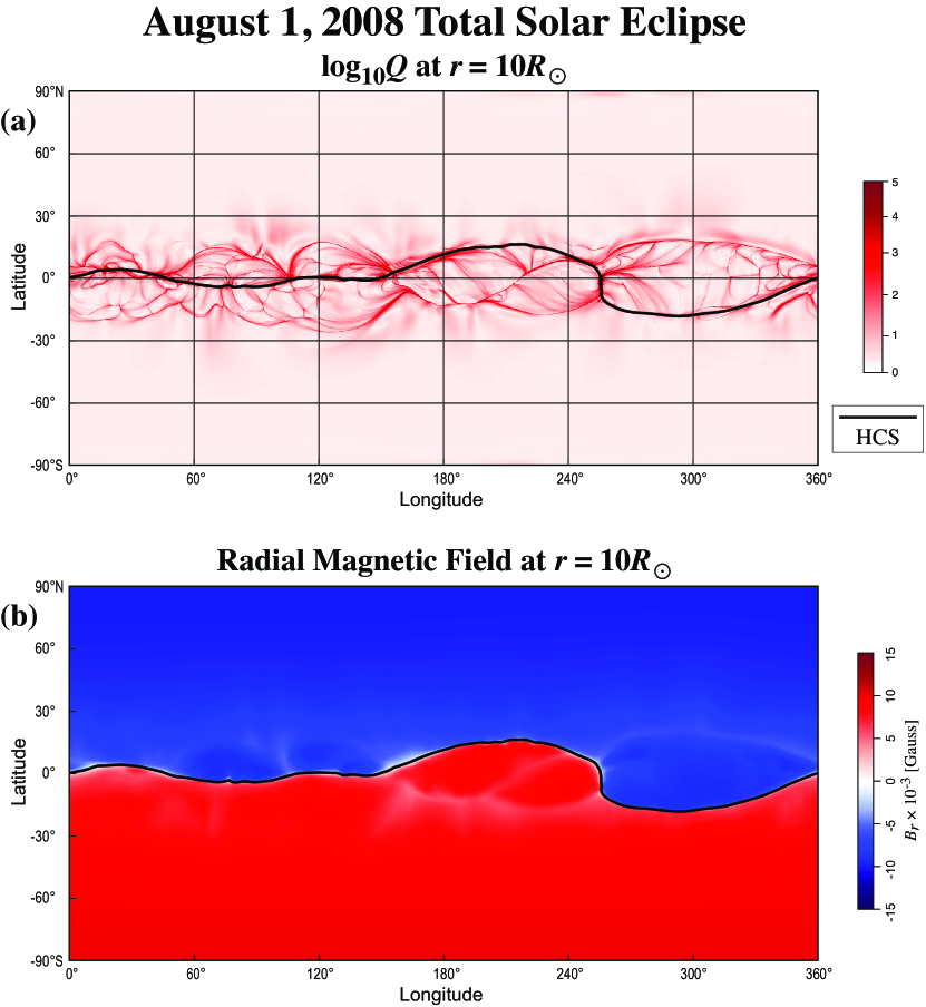
Figure 7a shows in the spherical surface at using a logarithmic scale. This is the structure that is expected to map into the inner heliosphere (appropriately wrapped into a spiral magnetic field by solar rotation), since the magnetic field has reached its asymptotic structure by this radius. The thick black line is the heliospheric current sheet (at which reverses sign). Figure 7b shows the magnitude of at the same radial surface . Note that the choice of is not crucial. Any surface in the heliosphere (where the field is all open) yields similar results.
It is important to emphasize that the apparent structure in expresses only the connectivity of the open field, not its actual magnitude. In spite of the enormous magnetic complexity at the solar surface, the radial field distribution in the heliosphere is completely unremarkable, Fig. 7b. There is a single polarity inversion line denoting a single HCS, as is generally observed near solar minimum, and this HCS runs more or less equatorial. The radial field is essentially uniform away from the HCS, as would be expected from simple pressure balance. (Careful examination of the plot of shows that there is a faint semblance of the structure that can be seen in , but it is only a small perturbation.)
On the other hand, the map at this surface is remarkable, indeed, Fig. 7a. We see that surrounding the HCS is a broad web of separatrices and QSLs of enormous complexity. There are at least four striking features of this S-web. First, it has an angular extent in latitude of approximately , sufficient to account for the observed extent of the slow wind. Note also that the angular extent does vary with longitude, but only by a factor of two or so. Second, the HCS is not necessarily in the center of the S-web, but is sometimes near its edge. This can explain the frequent observation that the HCS is usually not centrally located within slow wind streams (e.g., Burlaga et al., 2002). Third, the boundary between the S-web layer and the featureless polar hole region is sharp; it is narrow compared to the width of the S-web. This can explain the observation that the transition from slow to fast wind as measured by the composition data is narrow compared to the slow wind region itself (Zurbuchen et al., 1999).
In order to explore the details of how coronal hole extensions connect to the polar holes, we calculated coronal hole areas at different heights in the corona. Figure 8 shows the location of a region near longitude and latitude N in which we explored the connection between the low-latitude coronal hole extensions (of negative polarity, shown in blue) in detail. It is evident that the coronal hole extensions in this region appear disconnected from the north polar hole in the photosphere, but connect with it low in the corona (at heights approximately between and above the photosphere). Figure 9 shows explicitly how these coronal holes connect in the low corona. The three-dimensional shape of the coronal hole boundary is shown as a green semi-transparent surface in the low corona in the region detailed in Figure 8. This is the boundary between open and closed field regions. The regions marked by A, B, and C show examples in which the extensions of coronal holes are not connected in the photosphere, at least by any measurable open-field corridor, but appear to connect above the photosphere in the low corona. These regions are also indicated in Figure 8 for ease of cross-reference. Despite the fact that these coronal holes are “disconnected” in the photosphere, they always remain topologically linked in a singular manner with the polar coronal hole, as discussed by Titov et al. (2011).
Finally, note that the connections of the high- lines between the neighborhood of the HCS and the photosphere and low corona that were postulated by the uniqueness conjecture (Antiochos et al., 2007) are largely present, even though the insight from these new high-resolution MHD simulations has led us to generalize the uniqueness conjecture. We have found that, in general, coronal hole extensions are sometimes connected to the polar holes in the photosphere via narrow corridors, as originally postulated (Antiochos et al., 2007), but in other instances they are disconnected in the photosphere, but remain topologically linked to the polar holes (Titov et al., 2011). In either case, these connections are responsible for the formation of the S-web. It should be emphasized that in order to capture the intricate structure of these connections, very high resolution models are required that can incorporate some of the complexity of the photospheric magnetic carpet fields. Given sufficient resolution, the S-web should appear as a generic feature of all quasi-steady models, including the PFSS. In fact, the PFSS models should be more effective than the MHD for studying the complex topology of the S-web, because they allow for much higher spatial resolution than is possible with an MHD code. On the other hand, for quantitative comparison with observations, the MHD models should be more effective, because they include the gas thermal and kinetic pressure forces and Lorentz forces that we know are present in the real corona.
4 Discussion
The major conclusion from our results is that the underlying premise of the streamer top model is valid. The slow wind is expected to originate from the release of closed-field plasma due to the dynamic rearrangement of the open-closed field boundary. The key new addition of our S-web model to this picture is that the inherent complexity of the photospheric field leads to a network of narrowly connected and disconnected coronal holes that nevertheless always remain linked. This produces a separatrix web in the heliosphere that extends the release of slow wind to regions that significantly depart from the HCS. Hence, our model accounts for both the observed composition and the broad extent of the slow wind.
One immediate prediction from the model is that the angular width of the slow wind is determined primarily by the complexity of the flux distribution in the photosphere. This complexity produces a very convoluted polarity inversion line in the low corona and an intricate coronal hole pattern (Figure 5). Our ability to identify the S-web and its manifestations rests on high-resolution calculations that are beginning to capture the multitude of small dipoles in the photospheric magnetic field. If the solar field were a pure dipole, producing an inversion line that runs straight along the equator, then only the polar coronal holes would be present and there would be no separatrix web in the heliosphere. For this “basal” (though idealized) slow wind case, if we assume that the dynamic broadening of the open-closed boundary at the Sun is of order the scale of a supergranule, , the angular extent of the wind would be only of order –, and would be centered about the HCS. Of course, the solar field is never a simple dipole.
At the present time we do not know if the complexity seen in Figures 5–7 is typical, or whether it is particular to this late declining phase of Cycle 23. It should be noted that the present minimum appears to be somewhat different than the previous few minima. In particular, the polar field strength is significantly weaker (e.g., Luhmann et al., 2009).
The S-web model predicts that for time periods during which extensions of coronal holes away from the main polar holes are less prevalent than in Cycle 23, the angular extent of the slow wind region would be smaller. In fact, there is clear evidence from radio scintillation data (Tokumaru et al., 2010) and recent Ulysses solar wind measurements that the Cycle 23 minimum has a substantially broader and more structured slow wind region than that of the previous cycle. Indeed, during the previous minimum (circa 1996), equatorial coronal hole extensions were less common than during the recent solar minimum. Further high-resolution numerical calculations will be needed to address this result.
Another prediction of the model is that the slow wind region is actually a mixture of winds. It is evident from Fig. 7 that the separatrix web is not space-filling. There are regions within the broad S-web band where the wind emanates from the low-latitude coronal hole extensions. These regions are likely to have large expansion factor, so that the wind will be slow compared to the fast wind from the polar regions, but its composition will be different than that of closed-field plasma. Our model, therefore, naturally explains the observed variability of the slow wind composition.
A key aspect of the S-web model that has yet to be calculated is the dynamic release of closed-field plasma. Although our quasi-steady calculations allow us to investigate the topology of the field, and to identify the structure of the separatrix web in the heliosphere, they do not actually produce a slow wind with closed-field composition. For this we need fully dynamic simulations that include the driving due to photospheric motions (e.g., resulting from differential rotation) and flux emergence. Such simulations are now being performed in 3D (e.g., Edmondson et al., 2009, 2010; Linker et al., 2010) for simplified photospheric flux distributions and driving flows. These simulations do verify the basic idea of the S-web model that open-field corridors will form and evolve in response to photospheric motions (Edmondson et al., 2009). Higher resolution simulations will be needed, however, to test the model in detail. On the other hand, it seems unlikely that dynamic calculations with the degree of structure present in Fig. 7 will be feasible in the near future. It is likely that a definitive treatment of the slow wind will require the development of a statistical theory of the dynamics of the S-web model.
References
- Altschuler & Newkirk (1969) Altschuler, M. D. & Newkirk, G. 1969, Sol. Phys., 131
- Antiochos et al. (2007) Antiochos, S. K., DeVore, C. R., Karpen, J. T., & Mikić, Z. 2007, ApJ, 671, 936
- Bame et al. (1977) Bame, S. J., Asbridge, J. R., Feldman, W. C., & Gosling, J. T. 1977, J. Geophys. Res., 82, 148
- Bavassano et al. (1997) Bavassano, B., Woo, R., & Bruno, R. 1997, Geophys. Res. Lett., 24, 1655
- Bruno & Carbone (2005) Bruno, R. & Carbone, V. 2005, Living Reviews in Solar Physics, 2, no. 4, http://solarphysics.livingreviews.org/Articles/lrsp-2005-4/
- Burlaga et al. (2002) Burlaga, L. F., Ness, N. F., Wang, Y.-M., & Sheeley, N. R. 2002, J. Geophys. Res., 107(A11), 1410, doi:10.1029/2001JA009217
- Cranmer & van Ballegooijen (2005) Cranmer, S. R. & van Ballegooijen, A. A. 2005, ApJS, 156, 265
- Cranmer et al. (2007) Cranmer, S. R., van Ballegooijen, A. A., & Edgar, R. J. 2007, ApJS, 171, 520
- Crooker et al. (2004) Crooker, N. U., Huang, C.-L., Lamassa, S. M., Larson, D. E., Kahler, S. W., & Spence, H. E. 2004, J. Geophys. Res., 109, A03107, doi:10.1029/2003JA010170
- Démoulin et al. (1996) Démoulin, P., Henoux, J. C., Priest, E. R., & Mandrini, C. H. 1996, A&A, 308, 643
- Edmondson et al. (2009) Edmondson, J. K., Lynch, B. J., Antiochos, S. K., De Vore, C. R., & Zurbuchen, T. H. 2009, ApJ, 707, 1427
- Edmondson et al. (2010) Edmondson, J. K., Antiochos, S. K., De Vore, C. R., & Zurbuchen, T. H. 2010, ApJ, submitted
- Einaudi et al. (1999) Einaudi, G., Boncinelli, P., Dahlburg, R. B., & Karpen, J. T. 1999, J. Geophys. Res., 104, 521
- Endeve et al. (2004) Endeve, E., Holzer, T. E., &Leer, E. 2004, ApJ, 603, 307
- Feldman & Widing (2003) Feldman, U. & Widing, K. G. 2003, Space Sci. Rev., 107, 665
- Fisk et al. (1998) Fisk, L. A., Schwadron, N. A., & Zurbuchen, T. H. 1998, Space Sci. Rev., 86, 51
- Fisk (2003) Fisk, L. A. 2003, J. Geophys. Res., 108, 1157
- Fisk & Zhao (2009) Fisk, L. A. & Zhao, L. 2009, in Universal Heliospheric Processes, Proc. IAU Symp. 257, 109
- Geiss et al. (1995) Geiss, J., Gloeckler, G, & von Steiger, R. 1995, Space Sci. Rev., 72, 49
- Gosling (1997) Gosling, J. T. 1997, in AIP Conf. Proc. 385, Robotic Exploration Close to the Sun: Scientific Basis, ed. S. R. Habbal (Woodbury: AIP), 17
- Harvey (1985) Harvey, K. L. 1985, Aust. J. Phys., 38, 875
- Hoeksema (1991) Hoeksema, J. T. 1991, Adv. Space Res., 11, 15
- Kohl et al. (2006) Kohl, J. L., Noci, G., Cranmer, S. R., & Raymond, J. C. 2006, ARA&A, 13, 31
- Kovalenko (1981) Kovalenko, V. A. 1981, Sol. Phys., 73, 383
- Laming (2004) Laming, J. M. 2004, ApJ, 614, 1063
- Luhmann et al. (2009) Luhmann, J. G. et al. 2009, Sol. Phys., 256, 285
- Linker et al. (1999) Linker, J. A., Mikić, Z., Biesecker, D. A., Forsyth, R. J., Gibson, S. E., Lazarus, A. J., Lecinski, A., Riley, P., Szabo, A., & Thompson, B. J. 1999, J. Geophys. Res., 104, 9809
- Linker et al. (2010) Linker, J. A., Lionello, R., Mikić, Z., Titov, V. S., & Antiochos, S. K. 2010, ApJ, submitted
- Lionello et al. (2009) Lionello, R., Linker, J. A., & Mikić, Z. 2009, ApJ, 690, 902
- Marsch (2006) Marsch, E. 2006, Living Reviews in Solar Physics, 3, no. 1, http://solarphysics.livingreviews.org/Articles/lrsp-2006-1/
- McComas et al. (2000) McComas, D. J., Barraclough, B. L., Funsten, H. O., Gosling, J. T., Santiago-Munoz, E., Skoug, R. M., Goldstein, B. E., Neugebauer, M., Riley, P., & Balogh, A. 2000, J. Geophys. Res., 105, 10419
- McComas et al. (2008) McComas, D. J., et al. 2008, Geophys. Res. Lett., 35, L18103
- Meyer (1985) Meyer, J.-P. 1985, ApJS, 57, 173
- Mikić & Linker (1994) Mikić, Z., & Linker, J. A. 1994, ApJ, 430, 898
- Mikić et al. (1999) Mikić, Z., Linker, J. A., Schnack, D. D., Lionello, R., & Tarditi, A. 1999, Phys. Plasmas, 6, 2217
- Mikić et al. (2007) Mikić, Z., Linker, J. A., Lionello, R., Riley, P., & Titov, V. 2007, in Solar and Stellar Physics Through Eclipses, ASP Conference Series, Vol. 370, eds. O. Demircan, S. O. Selam, & B. Albayrak, (San Francisco: Astronomical Society of the Pacific), p.299
- Parker (1958) Parker, E. N. 1958, ApJ, 128, 664
- Parker (1963) Parker, E. N. 1963, Interplanetary Dynamic Processes, (New York: Interscience Publishers)
- Priest & Démoulin (1995) Priest, E. R., & Démoulin, P. 1995, J. Geophys. Res., 100, 23443
- Rappazzo et al. (2005) Rappazzo, A. F.,Velli, M., Einaudi, G., & Dahlburg, R. B. 2005, ApJ, 633, 474
- Rušin et al. (2010) Rušin, V., Druckmüller, M., Aniol, P., Minarovjech, M., Saniga, M., Mikić, Z., Linker, J. A., Lionello, R., Riley, P., & Titov, V. S. 2010, A&A, 513, A45
- Schatten et al. (1969) Schatten, K., Wilcox, J. W., & Ness, N. F. 1969, Sol. Phys., 9, 442
- Scherrer et al. (1995) Scherrer, P. H. et al. 1995, Sol. Phys., 162, 129
- Schrijver et al. (1997) Schrijver, C. J. et al. 1997, Nature, 48, 424
- Schwenn (1990) Schwenn, R., 1990, in Physics of the Inner Heliosphere I, eds. R Schwenn & E. Marsch, (Berlin:Springer-Verlag), p.99
- Sheeley et al. (1997) Sheeley, N. R., Jr. et al. 1997, ApJ, 484, 472
- von Steiger et al. (1995) von Steiger, R., Schweingruber, R. F., Wimmer, R., Geiss, J., & Gloeckler, G. 1995, Adv. Space Res.y, 15(7), 3
- von Steiger et al. (1997) von Steiger, R., Geiss, J., & Gloeckler, G. 1997, in Cosmic Winds and the Heliosphere, eds. J. R. Jokipii, C. P. Sonett, & M. S. Giampapa (Tucson: Arizona U Press), p. 581.
- von Steiger et al. (2000) von Steiger, R., et al., 2000, J. Geophys. Res., 105, 27217.
- von Steiger et al. (2001) von Steiger, R., Zurbuchen, T. H., Geiss, J., Gloeckler, G., Fisk, L. A., & Schwadron, N. A. 2001, Space Sci. Rev., 97, 123
- Suess et al. (1996) Suess, S.T., Wang, A-H. & Wu, S. T. 1996, J. Geophys. Res.101, 19957
- Titov et al. (1999) Titov, V. S., Démoulin, P., & Hornig, G. 1999, in Magnetic Fields and Solar Processes, ESA SP-448, 715T
- Titov et al. (2002) Titov, V. S., Hornig, G., & Démoulin, P. 2002, J. Geophys. Res., 107, 1164
- Titov (2007) Titov, V. S. 2007, ApJ, 660, 863
- Titov et al. (2008) Titov, V. S., Mikić, Z., Linker, J. A., & Lionello, R. 2008, ApJ, 675, 1614
- Titov et al. (2011) Titov, V. S., Mikić, Z., Linker, J. A., Lionello, R., & Antiochos, S. K. 2011, ApJ, in press
- Tokumaru et al. (2010) Tokumaru, M., Kojima, M., & Fujiki, K. 2010, J. Geophys. Res., 115(A4), 4102, doi:10.1029/2009JA014628
- Wang & Sheeley (1991) Wang, Y.-M., & Sheeley, N. R. 1991, ApJ, 372, L45
- Wang et al. (2000) Wang, Y.-M., Sheeley, N. R., Socker, D. G., Howard, R. A., & Rich, N. B. 2000, J. Geophys. Res., 105(A11), 25133
- Wang et al. (2007) Wang, Y.-M., Sheeley, N. R., Jr., & Rich, N. B. 2007, ApJ, 658, 1340
- Wang et al. (2009) Wang, Y.-M., Ko, Y.-K., & Grappin, R. 2009, ApJ, 691, 760
- Winterhalter et al. (1994) Winterhalter, D., Smith, E. J., Burton, M. E., Murphy, N., & McComas, D. J. 1994, J. Geophys. Res., 99(A4), 6667
- Zhao et al. (2009) Zhao, L., Zurbuchen, T. H., & Fisk, L. A. 2009, Geophys. Res. Lett., 36, CiteID L14104, doi:10.1029/2009GL039181
- Zirker (1977) Zirker, J. B. 1977, Coronal Holes and High Speed Wind Streams, (Boulder: Colorado Assoc. University Press)
- Zurbuchen et al. (1999) Zurbuchen, T. H., Hefti, S., Fisk, L. A., Gloeckler, G., & von Steiger, R. 1999, Space Sci. Rev., 87, 353
- Zurbuchen et al. (2002) Zurbuchen, T. H., Fisk, L. A., Gloeckler, G., & von Steiger, R. 2002, Geophys. Res. Lett., 29, 66, doi: 10.1029/2001GL013946
- Zurbuchen & von Steiger (2006) Zurbuchen, T. H., & von Steiger, R. 2006, in SOHO 17: 10 years of SOHO and Beyond, ed. H. Lacoste & B. Fleck, (Noordwijk, ESA), SP-617, p. 7.1
- Zurbuchen (2007) Zurbuchen, T. H. 2007, ARA&A, 45, 297