The EUV spectrum of the Sun: quiet and active Sun irradiances and chemical composition

We benchmark new atomic data against a selection of irradiances obtained from medium-resolution quiet Sun spectra in the EUV, from 60 to 1040 Å. We use as a baseline the irradiances measured during solar minimum on 2008 April 14 by the prototype (PEVE) of the Solar Dynamics Observatory Extreme ultraviolet Variability Experiment (EVE). We take into account some inconsistencies in the PEVE data, using flight EVE data and irradiances we obtained from Solar & Heliospheric Observatory (SoHO) Coronal Diagnostics Spectrometer (CDS) data. We perform a differential emission measure and find overall excellent agreement (to within the accuracy of the observations, about 20%) between predicted and measured irradiances in most cases, although we point out several problems with the currently available ion charge state distributions. We used the photospheric chemical abundances of Asplund et al. (2009). The new atomic data are nearly complete in this spectral range, for medium-resolution irradiance spectra. Finally, we use observations of the active Sun in 1969 to show that also in that case the composition of the solar corona up to 1 MK is nearly photospheric. Variations of a factor of 2 are present for higher-temperature plasma, which is emitted within active regions. These results are in excellent agreement with our previous findings.

1 Introduction

This paper is one of a series of studies where the EUV radiances and irradiances of the Sun are studied. One of the goals of these studies was the provision of well-calibrated EUV/UV irradiances of the quiet and active Sun, to aid the interpretation and modelling of stellar observations. As a first step on the modelling side, it is therefore important to assess the completeness and accuracy of current atomic data. This is the main aim of the present paper, where a large amount of recently-calculated atomic rates are included. We focus on quiet Sun irradiances, but also point out the differences with those of the more active Sun.

The present benchmark also provides a test on ion charge state distributions. In fact, to model full-Sun irradiances, it is well known that a continuous emission measure distribution is obtained. Therefore, lines of different ions formed at similar temperatures should have predicted irradiances close to the observed ones. Any discrepancies turn out to be mostly due to problems in the ion charge state calculations. Finally, the present benchmark also provides an excellent way to measure the chemical abundance of the solar transition region and corona.

An earlier assessment was carried out within the SOLID project, which aimed at providing and estimating the solar spectral irradiance across all wavelengths. Within SOLID, a comparative study between the EUV/UV spectral radiances/irradiances as observed by several instruments and as obtained with modelling using CHIANTI atomic data (Dere et al., 1997) was carried out. The earlier assessment was used to establish which atomic data needed improvement and which were missing, and ultimately led to a significant update of the CHIANTI database, version 8 (Del Zanna et al., 2015c).

As most of the issues discussed in the previous series of papers is relevant to the present analysis, we provide a brief summary: Paper I (Del Zanna et al., 2010) presented a new radiometric calibration of the Solar & Heliospheric Observatory (SoHO) Coronal Diagnostics Spectrometer (CDS; Harrison et al., 1995) Normal Incidence Spectrometer (NIS), which included earlier calibrations (Del Zanna et al., 2001; Brekke et al., 2000). In Paper I, quiet Sun NIS irradiances in 2008 were obtained and compared to those measured by a sounding rocket, flown on 2008 April 14 during the extended solar minimum, when the Sun was very quiet. The rocket carried a prototype (PEVE, see Woods et al. 2009) of the the Solar Dynamics Observatory (SDO) Extreme ultraviolet Variability Experiment (EVE, see Woods et al. 2012), and produced a medium-resolution EUV spectrum over a broad spectral range (60–1040 Å). Very good agreement between the NIS and PEVE irradiances for most of the lines was found. However, problems in the PEVE irradiances in some of the strongest lines were found. This was surprising as the PEVE instrument was radiometrically calibrated on the ground (Chamberlin et al., 2007; Hock et al., 2010; Chamberlin et al., 2009).

Our new SoHO CDS calibration allowed the first measurements of the EUV spectral irradiance along a solar cycle, from 1998 until 2010, which was presented in Paper II (Del Zanna & Andretta, 2011). The irradiances in lines formed below 1 MK were shown to vary little, with the exception of the He lines. A new calibration for the most prominent line in the EUV, the He ii 304 Å resonance transition, was proposed. The change was significant, and implied that most previous calibrated values were incorrect by about a factor of two. Our new NIS calibration was later confirmed by a sounding rocket flight, EUNIS (see Wang et al. 2011). Paper III (Andretta & Del Zanna, 2014) analysed in detail the radiances and limb-brightening in the main lines and their variation with the solar cycle. Paper IV (Del Zanna et al., 2015a) compared the CDS irradiances with the count rates measured by the Solar EUV Monitor (SEM) first-order band (SEM 1). Paper V (Del Zanna & Andretta, 2015) extended and revised the CDS NIS calibration until 2014 when the instrument was switched off. The irradiances obtained from this analysis were then compared to those measured by PEVE, by SDO EVE and by the Thermosphere Ionosphere Mesosphere Energetics Dynamics (TIMED) Solar EUV Experiment (SEE) EUV Grating Spectrograph (EGS) (Woods et al., 2005). Excellent agreement (to within a relative 10–20%) with the EVE data (only during the 2010–2012 period) was found; however, the problems in the PEVE irradiances were confirmed, and several discrepancies with the TIMED EGS irradiances were also found.

The present assessment is the first of its kind in the EUV as briefly pointed out below in Section 2. Section 3 briefly describes the new atomic data used in the present paper, while Section 4 presents the quiet Sun irradiances, a differential emission measure (DEM) modelling and predicted spectra. Section 5 revisits older irradiance observations of the active Sun, while Section 6 draws the conclusions.

2 Previous benchmark studies in the EUV

Several assessments of atomic data in the EUV have been carried out previously, but on radiances in narrow wavelength ranges or in specific ions. For example, in a long series of papers starting with Del Zanna et al. (2004), the atomic data of several key ions have been benchmarked against laboratory and astrophysical spectra, providing many lacking identifications in the EUV, as reviewed in Del Zanna & Mason (2018). Most of these identifications have been included in CHIANTI version 7.1 and 8.

A significant benchmark study based on the first SERTS rocket flight (Thomas & Neupert, 1994) was carried out by Young et al. (1998) in the 170-450 Å range. The most complete previous assessment of atomic data for the EUV used SoHO CDS NIS and grazing incidence (GIS) radiances in the 150–780 Å range (Del Zanna, 1999), but was limited by an uncertain CDS radiometric calibration and the use of older CHIANTI atomic data.

Landi et al. (2002) also performed a benchmark of CHIANTI data for the coronal lines using off-limb observations from CDS NIS. An assessment of more recent CHIANTI atomic data in the 166–212 Å and 245–291 Å spectral ranges observed by the Extreme-ultraviolet Imaging Spectrometer (EIS, see Culhane et al. 2007) aboard Hinode was carried out in Del Zanna (2012b) on coronal lines. Del Zanna (2009a) and Landi & Young (2009) benchmarked CHIANTI atomic data for transition-region lines observed by EIS.

SoHO Solar Ultraviolet Measurements of Emitted Radiation (SUMER, Wilhelm et al. 1995, 700–1600 Å) quiet Sun radiances were compared with earlier CHIANTI atomic data by Doschek et al. (1999), finding significant discrepancies. We note, however, that the lack of simultaneity in observing SUMER lines far apart in wavelength is a limiting issue for this type of studies, considering that the dominant lines are highly variable. An improvement was the benchmark of CHIANTI data for coronal lines using quiet Sun off-limb SUMER observations by Landi et al. (2002), as these lines normally show little variability.

3 Atomic data, ion and elemental abundances

Within the UK APAP network, we have carried out over the past few years several large-scale structure and scattering $R$-matrix calculations to produce atomic data for dozens of ions (see the review in Badnell et al., 2016). The present author has carried out a series of calculations, briefly listed in Del Zanna & Mason (2018), that have greatly improved the atomic data for coronal ions. The main ions producing the majority of spectral lines in the EUV and soft X-rays are from iron: Fe viii (Del Zanna & Badnell, 2014), Fe ix (Del Zanna et al., 2014), Fe x (Del Zanna et al., 2012a), Fe xi (Del Zanna & Storey, 2013), Fe xii (Del Zanna et al., 2012b), Fe xiii (Del Zanna & Storey, 2012), and Fe xiv (Del Zanna et al., 2015b). The UK APAP data have been included in CHIANTI Version 8 (Del Zanna et al., 2015c).

For the present assessment, we use as a baseline CHIANTI v.8, plus a few minor changes that are being released within CHIANTI v.9 (Dere et al., 2019) and a large set of new atomic data that have been prepared for CHIANTI v.10 (Del Zanna et al., in preparation). These include APAP data for all the Be-like (Fernández-Menchero et al., 2014a) and Mg-like (Fernández-Menchero et al., 2014b) ions. New data for several ions have also been included: S iv (Del Zanna & Badnell, 2016a), Fe xiv (Del Zanna et al., 2015b), Ni xii Del Zanna & Badnell (2016b). Radiative rates from a selection of sources were also added.

3.1 The ion charge states at zero density

During the course of the present assessment we have tested several ion charge state distributions (ion abundances), calculated assuming ionization equilibrium at zero-density (the coronal approximation), i.e. assuming that all the population in an ion is in the ground state. The tables published in CHIANTI v.6 (Dere et al., 2009) are a significant improvement over previous ones, because of new ionization rates (Dere, 2007), radiative recombination rates (Badnell, 2006), and dielectronic recombination rates (see Badnell et al. 2003 and the series of following papers).

The recombination rates for some ions were subsequently revised in CHIANTI v.7.1 (Landi et al., 2013). They mostly affected the charge state distribution of a few iron and nickel coronal ions, most notably Fe viii and Fe ix. When using the CHIANTI v.7.1 charge state distributions we obtained predicted irradiances about a factor of two higher than observed, for both Fe viii and Fe ix. It turned out that the large discrepancies were due to errors in the recombination rates of Fe viii and Fe ix in CHIANTI. These were corrected and released in v.8.07, which we use here.

3.2 Anomalous ions and ion charge states with density effects

The Li- and Na-like ions give rise to some of the strongest lines in the EUV/UV spectral region. However, many of these ions are anomalous, in that the emission measures obtained from them are at odds with those obtained from ions of other isoelectronic sequences. This was first noted by Burton et al. (1971), although even earlier observations present the same problem, as described in Del Zanna & Mason (2018). Del Zanna et al. (2002) showed for the first time that the same problem is common in stars other than the Sun.

The issue of anomalous ions has been largely neglected in the literature, and there is still no obvious explanation, although several effects could be at play. Departures from ionization equilibrium can enhance significantly some of the ions that have long ionization/recombination times, as shown e.g. in Bradshaw et al. (2004). Non-Maxwellian electron distributions tend to shift the formation temperature of the TR lines towards lower values, leading to an enhancement, as shown for the Si iv case by Dudík et al. (2014).

However, various effects related to the density of the plasma are always going to be present. One is a suppression of the dielectronic recombination, as described in Burgess & Summers (1969). The authors developed a collisional-radiative modelling (CRM) which was further improved and implemented within the Atomic Data and Analysis Structure (ADAS), the consortium for fusion research. We have started a programme of new atomic calculations to model these and other (e.g. photo-ionization) effects with up-to-date rates (Dufresne & Del Zanna, 2018), but for the present paper we have tested the ion fractions calculated using the effective rates as available in OPEN-ADAS, which include density effects.

The helium lines (neutral and singly-ionized) are also much stronger than predicted by large factors, an issue that has been discussed extensively in the literature. There are various processes that could lead to enhancements of these lines. Recombination following photo-ionization from coronal radiation is one of those (see, e.g. Andretta et al. 2003 and references therein). Non-equilibrium effects such as time-dependent ionization (see, e.g. Bradshaw et al. 2004) and diffusion processes (see, e.g. Fontenla et al. 1993), are also important. A recent study by Golding et al. (2017) showed that time-dependent ionization, recombination and radiative transfer effects can indeed increase the intensities of the helium lines by a factor of 10. We provide no attempt here to model lines from He nor from H, and point out that in general radiative transfer effects should be considered when modelling some of the lines in neutral and singly ionized atoms.

3.3 Coronal abundances of the quiet Sun are photospheric!

Measurements of elemental abundances and temperatures are closely linked, since the DEM distribution can be used to both describe the temperature distribution of the plasma and obtain relative elemental abundances (see the review of the methods in Del Zanna & Mason, 2018). It is well known that solar coronal abundances present variations and differ from the photospheric ones, although there is a significant amount of controversy in the literature. The ratio of the coronal abundances of the low ($\leq$ 10 eV) first ionization potential (FIP) elements vs. the high-FIP ones is often higher than the photospheric value (the so-called FIP bias). Controversy in the literature regards the significant revision of the abundances of several important high-FIP elements (e.g. carbon, oxygen) proposed by Asplund et al. (2009).

There is now sufficient evidence that chemical abundances in the quiet Sun transition-region are photospheric, while controversial results about the FIP bias in the corona have been published (see the reviews by Laming, 2015; Del Zanna & Mason, 2018). Recent analyses of SoHO SUMER (Del Zanna & DeLuca, 2018) and UVCS (Del Zanna et al., 2018) using CHIANTI v.8 of quiet Sun areas show excellent agreement with the Asplund et al. (2009) photospheric abundances, mostly because of the significant differences in the v.8 atomic data compared to earlier ones. We therefore use these photospheric abundances for the present analysis. We return to the issue of chemical abundances below, when we present an analysis of the active Sun.

4 The quiet Sun irradiances

We use the PEVE spectrum as the basis for our study of the quiet Sun irradiances, because it was taken during the extended solar minimum. The solar radio F10.7 flux was 69. The Sun was mainly featureless, with a polar coronal hole and a very small active region, which affected somewhat a truly ‘quiet Sun’ measurement.

As shown in Paper V, several of the strong lines have PEVE irradiances that are much higher than those measured by CDS NIS, and also higher than the values measured in May 2010 by the in-flight EVE instrument (we considered the version 5 data). We have therefore studied the EVE daily irradiances during May–June 2010 to see if a relatively quiet period could be found. We considered the F10.7 radio flux and looked at the variation of the EVE irradiances. We selected 2010 May 16 as one of the best dates. Unfortunately, the Sun already had five small active regions on the visible side, and indeed all the irradiances of the lines formed above 1 MK are significantly enhanced in the 2010 May 16 EVE spectrum, compared to the PEVE spectrum, despite the fact that the F10.7 radio flux was only 70. On a side note, this comparison clearly shows that the F10.7 radio flux is not a good indicator of very low levels of solar activity.

We have measured the irradiances of both the EVE and PEVE lines subtracting a background, but note that this background subtraction only affects the measurements of the main lines by at most 10%, as shown in Paper V.

The discrepancies between the PEVE and EVE observations are sometimes significant (50%), well above the quoted uncertainties, and cannot be due to solar variability for lines formed below 1 MK. In fact, all the low-temperature emission lines (except the helium lines) have a very small variation during the solar cycle, as shown in Paper II and Paper III. The differences can only be due to calibration problems. To aid the assessment, we have considered all the historical records of EUV irradiances, as carried out previously in Paper II. We have also considered our CDS NIS irradiances during solar minimum to assess when the PEVE values were reasonable. In a few cases, we have replaced the PEVE irradiances with the EVE measurements. The irradiances of a selection of EUV lines are given in Table 1, where other measurements for some of the cooler lines are also provided. We only list those measurements we regard as relatively accurate: our CDS NIS measurements of 2008 Sept 22, and the irradiances published by Malinovsky & Heroux (1973) and Heroux et al. (1974). The F10.7 radio flux on 2008 Sept 22 was 69.6 and the Sun only had a small active region, i.e. was very quiet. Malinovsky & Heroux (1973) published a calibrated spectrum in the 50-300 Å range with a medium resolution (0.25 Å), taken with a grazing-incidence spectrometer flown on a rocket on 1969 April 4, when the F10.7 flux was 177.3, i.e. when the Sun was ‘active’, and significant contributions from active regions and flares were present. Heroux et al. (1974) provided irradiances also obtained from a sounding rocket flown in 1972 August 23 when the F10.7 flux was 120, i.e. the Sun was moderately active. A more extended list of EUV quiet Sun irradiances is provided in Table A in the Appendix.

4.1 DEM and predicted irradiances

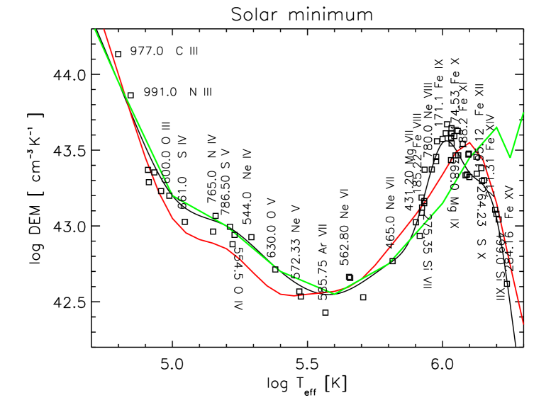
Figure 1: The volume DEM distribution of the quiet Sun. The points indicate the ratio of the predicted vs. observed irradiance, multiplied by the DEM value at the effective temperature. The labels indicate the wavelength ( Å) and the main ion. The red line indicate the DEM obtained from the CDS NIS measurements of 2008 Sept 22, while the green line the DEM obtained from the active Sun using the Malinovsky & Heroux (1973) irradiances.

A DEM modelling was carried out, exploring a range of parameters. We used the Del Zanna (1999) method, whereby the DEM is modeled as a spline distribution. The intensity of the vast majority of the strongest spectral lines is largely independent of the density, however some transition region lines are sensitive to the varying density in the lower part of the solar atmosphere. An example is the O v multiplet at 760 Å. We adopted a model with a constant pressure of 5$\times$10¹⁴ cm^-3 K^-1 and the CHIANTI v.8.07 zero-density ion abundances. The resulting volume DEM is shown in Fig. 1. To indicate how well the DEM is constrained, we also plot in Fig. 1 the ratio of the predicted vs. observed irradiance, multiplied by the DEM value at the effective temperature

$$T_{\rm eff}={\int T\leavevmode\nobreak\ G{\left({T}\right)}\leavevmode\nobreak\ DEM{\left({T}\right)}\leavevmode\nobreak\ dT\over\int G{\left({T}\right)}\leavevmode\nobreak\ DEM{\left({T}\right)}\leavevmode\nobreak\ dT}$$ (1)

which is an average temperature more indicative of where a line is formed. This is often quite different than $T_{\rm max}$, the temperature where the $G(T)$ of a line has a maximum.

For comparison, we show in Fig. 1 the DEM obtained from the CDS NIS irradiances of 2008 Sept 22 (cf. Paper IV). There is overall agreement, as expected. We stress that, as noted in Paper IV, all the DEM distributions that we have obtained from NIS along the solar cycle are all similar below 1 MK, because of the little variation in the irradiances of the cooler lines.

The irradiances predicted using the DEM and the zero-density ion abundances are also listed in Table 1. In most of the cases, using the same DEM and the ion abundances calculated from OPEN-ADAS at a constant pressure of 5$\times$10¹⁴ cm^-3 K^-1, we obtain similar irradiances, but note that the density effects tend to shift the formation temperature of a transition-region ion towards lower values. However, in a number of cases, significant discrepancies are present. We only list the main discrepancies in Table 1.

Table 1: Observed and predicted quiet Sun EUV irradiances for transition-region lines, for increased formation temperature.

$\lambda_{\rm obs}$	$I_{\rm obs}$	$T_{\rm max}$	$T_{\rm eff}$	$R$	Ion	$\lambda_{\rm exp}$	$r$
(Å)		(log)	(log)			(Å)
1036.54	3.1	4.65	4.55	2.70	C ii	1036.337	0.33
					C ii	1037.018	0.66
	4.4 (EVE)
ADAS		4.48	4.44	1.32	C ii
977.04	51.4	4.94	4.80	0.66	C iii	977.020	0.99
	46 (H74), 60 (EVE)
ADAS		4.82	4.69	0.97	C iii
991.60	3.4	4.94	4.85	0.77	N iii	991.577	0.87
	3.9 (H74), 3.7 (EVE)
599.59	1.5	5.02	4.99	1.07	O iii	599.590	0.99
	1.6 (H74), 1.2 (EVE, CDS)
661.40	0.25	5.06	5.05	1.24	S iv	661.420	0.88
	0.37 (PEVE)
ADAS		5.03	4.97	1.41	S iv
489.48	0.15	5.06	5.15	1.18	Ne iii	489.495	0.79
					Ne iii	489.629	0.15
ADAS		4.94	5.09	0.89	Ne iii
765.11	3.7	5.18	5.16	0.92	N iv	765.152	0.98
	2.0 (H74), 2.8 (EVE)
786.49	1.5	5.22	5.21	0.98	S v	786.468	0.98
	1.3 (H74), 1.3 (EVE)
ADAS		5.16	5.16	0.69	S v
554.39	5.5	5.22	5.23	1.06	O iv	554.076	0.27
					O iv	554.514	0.70
	6.8 (H74), 5.1 (EVE), 5.9 (CDS)
543.87	0.25	5.25	5.29	0.89	Ne iv	543.886	0.97
	0.30 (CDS)
629.73	13.9∗	5.39	5.38	1.04	O v	629.732	0.98
	12.6 (MH73), 16 (H74), 17.7 (PEVE), 8.8 (CDS)
ADAS		5.33	5.32	0.75	O v
572.29	0.31	5.43	5.47	1.10	Ne v	572.336	0.84
					Ne v	572.113	0.13
	0.28 (CDS)
585.67	0.13∗	5.55	5.57	1.32	Ar vii	585.748	0.79
	0.21 (PEVE)
562.78	0.61	5.60	5.65	0.82	Ne vi	562.805	0.81
					Ne vi	562.711	0.17
	0.45 (CDS)
401.85	0.66	5.61	5.66	0.84	Ne vi	401.941	0.97

Table 1: Observed and predicted quiet Sun EUV irradiances for upper transition-region lines.

$\lambda_{\rm obs}$	$I_{\rm obs}$	$T_{\rm max}$	$T_{\rm eff}$	$R$	Ion	$\lambda_{\rm exp}$	$r$
(Å)		(log)	(log)			(Å)
465.17	2.6∗	5.72	5.82	1.00	Ne vii	465.221	0.98
	2.6 (H74), 3.3 (PEVE)
ADAS		5.68	5.75	0.39	Ne vii	465.221
431.26	0.27	5.79	5.90	0.96	Mg vii	431.319	0.77
					Mg vii	431.194	0.21
168.10	0.77	5.71	5.92	1.43	Fe viii	168.929	0.11
					Fe viii	168.544	0.21
					Fe viii	168.172	0.35
					Fe viii	167.486	0.22
	0.95 (MH73), 0.80 (EVE)
429.08	0.10	5.79	5.92	0.88	Mg vii	429.140	0.92
185.29	0.35	5.71	5.92	1.12	Fe viii	185.213	0.88
	0.44 (MH73), 0.26 (EVE)
278.40	0.33	5.80	5.92	1.05	Mg vii	278.404	0.63
					Si vii	278.450	0.30
	0.34 (MH73), 0.36 (H74), 0.27 (EVE)
681.81	0.15	5.94	5.93	1.11	Na ix	681.719	0.78
					S iii	681.488	0.18
	0.25 (PEVE)
275.42	0.35	5.80	5.93	1.08	Si vii	275.361	0.84
					Si vii	275.676	0.14
	0.28 (MH73), 0.25 (H74), 0.26 (EVE)
ADAS		5.73	5.88	0.48	Si vii
466.10	0.45	5.81	5.93	0.68	Ca ix	466.240	0.98
411.15	0.23	5.87	5.94	0.53	Na viii	411.171	0.93
780.31	2.1	5.80	5.96	1.01	Ne viii	780.385	0.95
	1.8 (MH73) 1.9 (H74), 2.5 (PEVE)
ADAS		5.74	5.92	0.79	Ne viii
315.07	1.1	5.91	5.98	1.03	Mg viii	315.015	0.97
	1.35 (CDS)
430.41	0.75	5.91	5.98	0.84	Mg viii	430.454	0.97
170.98	7.0	5.91	6.00	0.95	Fe ix	171.073	0.99
	4.4 (MH73), 4.2 (H74), 3.95 (EVE)
319.86	1.4	5.94	6.01	0.89	Si viii	319.840	0.98
	1.38 (CDS)
ADAS		5.87	5.97	0.66	Si viii
706.05	0.52	5.99	6.02	0.78	Mg ix	706.060	0.95
	0.34 (EVE)
557.60	0.26	5.89	6.03	1.30	Ca x	557.766	0.99
	0.21 (CDS)
368.10	5.8∗	5.99	6.03	0.86	Mg ix	368.071	0.96
	6.2 (H74) 8.1 (PEVE), 5.8 (CDS)
272.05	0.42	5.28	6.03	0.79	Si x	271.992	0.75
443.80	0.25	5.99	6.03	1.00	Mg ix	443.404	0.16
					Mg ix	443.973	0.78
198.51	0.26	5.96	6.04	0.84	S viii	198.554	0.65
					Fe xi	198.538	0.27
	0.23 (MH73), 0.24 (EVE)

Table 1: Observed and predicted quiet Sun EUV irradiances for coronal lines.

$\lambda_{\rm obs}$	$I_{\rm obs}$	$T_{\rm max}$	$T_{\rm eff}$	$R$	Ion	$\lambda_{\rm exp}$	$r$
(Å)		(log)	(log)			(Å)
345.13	0.90	6.06	6.06	0.72	Si ix	345.121	0.74
					Si ix	344.954	0.21
	1.37 (CDS)
174.57	3.7	6.05	6.06	1.03	Fe x	174.531	0.98
	4.6 (MH73), 4.1 (H74), 3.8 (EVE)
624.94	2.1	6.07	6.07	0.76	Mg x	624.968	0.92
	1.4 (CDS)
148.38	0.38	6.11	6.08	1.14	Ni xi	148.377	0.99
	0.59 (H74), 0.45 (EVE)
188.29	2.3	6.13	6.09	1.08	Fe xi	188.216	0.50
					Fe xi	188.299	0.31
					Fe ix	188.493	0.13
178.09	0.14	6.12	6.10	0.78	Fe xi	178.058	0.91
180.41	2.7	6.13	6.10	1.07	Fe xi	180.401	0.84
264.30	0.38	6.18	6.13	0.71	S x	264.231	0.98
152.05	0.11	6.24	6.14	0.80	Ni xii	152.151	0.94
	0.36 (H74), 0.23 (EVE)
195.09	1.4	6.20	6.15	0.96	Fe xii	195.119	0.95
202.10	0.96	6.25	6.15	0.92	Fe xiii	202.044	0.64
					Fe xi	202.424	0.12
211.40	0.33	6.29	6.19	0.97	Fe xiv	211.317	0.75
					Ni xi	211.430	0.12
499.41	0.34	6.29	6.20	0.95	Si xii	499.406	0.94
ADAS		6.24	6.18	2.14	Si xii
284.12	0.46	6.34	6.24	1.05	Al ix	284.042	0.20
					Fe xv	284.163	0.76

The present results in terms of anomalous ions differ in some respect with the earlier ones. In fact, the irradiances of the higher-temperature lines, the Li-like Ne viii, Na ix, Mg x, Si xii are well represented, unlike many previous reports. The reasons could be due to the better instrument calibration, and the fact that we are analysing the solar irradiance during the solar minimum. When active regions are present, non-equilibrium effects are likely to become stronger.

For some low-temperature ions such as C ii and C iii (as well as the anomalous ion C iv, not shown here), the OPEN-ADAS rates provide a significant improvement over the zero-density ones. However, in many cases significant discrepancies are present. The most obvious ones are those for the strong Ne vii, Si vii, and Si xii where the predicted irradiances are off by a factor of two. The problems are present also if the ADAS data are used to infer a DEM. It is impossible to ascertain the reasons for such discrepancies, given that information on the basic rates used in the ADAS CRM is not available.

4.2 Quiet Sun EUV spectra

The DEM and the same set of parameters used for the inversion were then used to produce a modeled spectrum, to be compared to the observed one, to assess for completeness in the atomic data. The PEVE quiet Sun spectrum of 2008 is shown in Fig. 2 in black, while the quiet Sun EVE spectrum on 2010 May 16 is in grey. Fig. 2 shows that any small solar activity affects significantly the solar spectrum at most wavelengths. The predicted line profiles are approximated with Gaussians and shown in red in Fig. 2, while the positions and intensities of the main contributing lines are shown by vertical blue lines. We recall that several PEVE irradiances are not correct, and that lines from H and He are notoriously difficult to model. We now briefly summarise the main findings for each wavelength region.

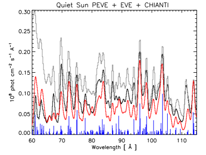
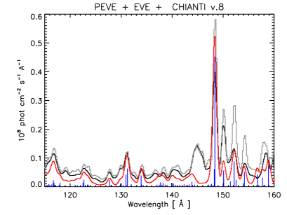
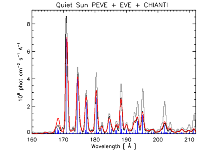
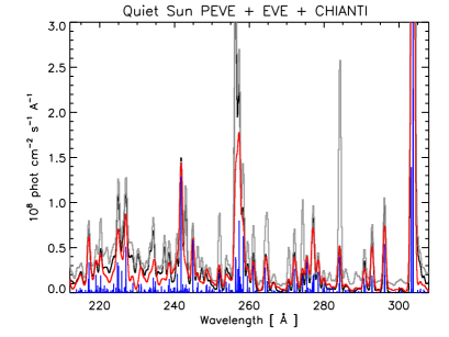
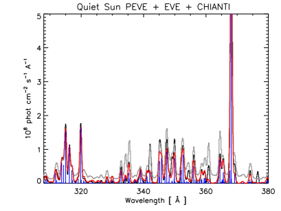
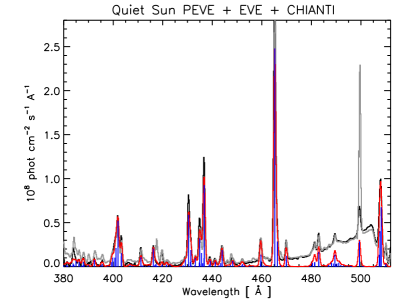
Figure 2: Observed PEVE quiet Sun spectrum in 2008 (black), with the observed EVE spectrum on 2010 May 16 (grey) and the predicted spectrum (red). The positions and intensities of the main contributing lines are shown by vertical blue lines.

4.2.1 The soft X-rays: 60–160 Å

As shown in Fig. 2, relatively good agreement with the PEVE data is found, although further work is still needed in this relatively unexplored spectral region. When calculating the atomic data for the coronal iron ions, we were surprised to find that many lines have increased intensities, when compared to distorted wave calculations (available since CHIANTI v.7.1, see Landi et al. 2013). This was due to resonance enhancements in the excitation rates and cascading effects. These new atomic data and identifications have been included in CHIANTI v.8 and allowed the first identifications of the strongest iron coronal lines in this spectral region, using much higher-resolution solar and laboratory spectra (Del Zanna, 2012a).

4.2.2 The 160–310 Å spectral region

Most of the 160–290 Å spectral region is now well understood, after several studies based on the Hinode EIS spectra (cf. Del Zanna, 2012b), and the new atomic data previously mentioned. The agreement between theory and observations is within a few percent, with the exception of one of the Fe viii lines at 168.7Å and the strong Fe ix resonance line at 171 Å. As we have previously mentioned, the disagreement is much larger when considering CHIANTI ion abundances earlier than 8.0.7.

We note that the PEVE irradiances of the Fe viii lines around 168Å are in good agreement with the EVE and Malinovsky & Heroux (1973) ones and several weaker Fe viii lines at longer wavelengths are very well reproduced. All the Fe viii EUV lines were benchmarked against high-resolution solar and laboratory observations (Del Zanna, 2009b), showing good agreement.

We also note an inconsistency in the measured irradiances of the Fe ix 171 Å line. As shown in Table 1, the PEVE irradiance is 7.0 (10⁸ photons cm^-2 s^-1 arcsec^-2) while the EVE v.5 value is much lower, 3.95. The Malinovsky & Heroux (1973) value is 4.4. Excellent agreement with theory is found when using the PEVE value. We note that all the other Fe ix lines at longer wavelengths, most notably the two density-sensitive lines at 241.74 and 244.91 Å, are also very well reproduced.

In an earlier benchmark (Del Zanna et al., 2011), we showed that several coronal lines in the 205–240 Å are still unidentified, so further work is needed in this spectral region. This can also be seen looking at Table A, although these missing lines are not very strong in solar irradiance spectra. Aside from this region, good agreement is found, as Fig. 2 shows. One exception is the series of He ii lines at 304, 256, 243 Å.

4.2.3 The 310-380 Å spectral region

The 310-380 Å spectral region is also well reproduced, as significant effort in improving the atomic data was produced before the launch of SoHO, as shown by the earlier atomic benchmark studies using the SoHO CDS NIS 1 spectra (Del Zanna, 1999). Many of the lines in this spectral region are due to coronal iron ions, for which the new atomic data in CHIANTI v.8 are a significant improvement. For several iron lines in this band enhancements of about 30% are present. This is caused by resonance enhancement and cascading effects increasing the decays from the lower levels producing the lines in this spectral region.

4.2.4 The 380–510 Å spectral region

The quiet Sun spectrum in the 380–510 Å  region is dominated by transition-region lines from Ne and Mg ions. This spectral region is also well understood, because various studies based on the SoHO CDS GIS spectra were performed (Del Zanna, 1999), and because the atomic data for the ions in this spectral range are relatively easier to calculate. Fig. 2 shows that there is very good agreement between observed and predicted irradiances. We note that the neutral helium continuum (with the edge at 504 Å) cannot be modeled properly without taking into account radiative transfer effects.

4.2.5 The 510-630 Å spectral region

The 510-630 Å spectral region is also well known and complete in terms of atomic data, since SoHO CDS NIS 2 spectra have been used to benchmark the atomic data (Del Zanna, 1999), and most of the ions are low charge. Very good agreement is found, with the exception of the series of He i lines.

4.2.6 The 630-780 Å spectral region

The 630-780 Å spectral region has been studied using CDS GIS spectra (Del Zanna, 1999). Good overall agreement between observed and predicted line irradiances is found. We note that the intensities of the O ii 718 Å line and of the O v multiplet at 760 Å are very sensitive to the temperatures and densities of the model. With the present atomic data, the O v multiplet is well represented, but the O ii line is not. Using the ADAS ion abundances for O ii does not improve the comparison. We also note that the hydrogen continuum (with the edge at 912 Å) cannot be modeled properly without taking into account radiative transfer effects.

4.2.7 The 780–912 Å spectral region

The few O iii and O iv in this wavelength region are well represented (cf. Table A), but all the O ii lines are incorrectly modeled (also using the ADAS ion abundances).

4.2.8 The 912–1045 Å spectral region

The C iii resonance line at 977 Å is relatively well represented with the CHIANTI v.8.0.7 ion fractions, although the ADAS ion abundances improve agreement. The N iii 991.57 Å line is also well represented (cf. Table A). The doublet at 1031.9, 1037.6 Å from the anomalous ion O vi is under-predicted by more than a factor of 2. Only a small improvement is obtained using the ADAS ion abundances.

5 The active Sun irradiances and chemical abundances

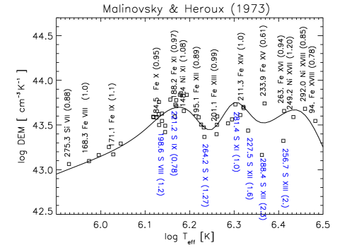
Figure 3: The DEM distribution obtained from the active Sun Malinovsky & Heroux (1973) irradiances. The points indicate the ratio of the predicted vs. observed irradiance, multiplied by the DEM value at the effective temperature. The labels indicate the wavelength (Å), main ion, and the ratio of the predicted vs. observed irradiance (in brackets).

The Laming et al. (1995) study, based on the Malinovsky & Heroux (1973) spectrum, is often cited in the literature to support the argument that the solar corona has a FIP bias of about 4. However, Laming et al. (1995) clearly stated that nearly photospheric abundances were found when considering lines formed in the transition region, up to 1 MK. The FIP bias of 3–4 was obtained from higher-temperature lines. Clearly, this hot emission would be significantly biased by the active regions and not the quiet Sun, where almost no emission above 1 MK is present.

So, to interpret the full-Sun spectra such as those of Malinovsky & Heroux (1973) we need to have a good understanding of the abundances in active regions. Controversial results about the FIP bias in the hot (3 MK) cores of active regions have been published in the literature. However, a recent revision of EUV (Hinode/EIS) and X-ray (SMM/FCS) measurements of several active regions have indicated a remarkable consistency, with an FIP bias of about 3.2 (Del Zanna, 2013b; Del Zanna & Mason, 2014). Del Zanna (2013b) also showed that it must be the low-FIP elements that are enhanced by at least a factor of 3, compared to the photospheric values. Note that the Del Zanna (2013b) results were obtained using a new Hinode EIS calibration (Del Zanna, 2013a).

Considering the significant updates in atomic data since the Laming et al. (1995) study, and the changes in the photospheric abundances recommended by Asplund et al. (2009), it is worth reconsidering the well-calibrated Malinovsky & Heroux (1973) EUV irradiances. We have chosen a selection of lines in the Malinovsky & Heroux (1973) EUV spectrum, avoiding the lines strongly density-dependent. We note that in several cases, the authors had deblended the intensities of lines close in wavelength. The spectrum must have been obtained after or during flaring emission, as the Fe xviii line at 93.9 Å was relatively strong. We have taken the deblended value as recommended by Malinovsky & Heroux (1973) but applied a correction factor of 2 to its irradiance, following the problems in the soft X-rays described in Del Zanna (2012a). With this correction, good agreement between predicted and observed irradiance is obtained.

We used the set of atomic data previously described, the CHIANTI v.8.07 zero-density ion abundances, and the Asplund et al. (2009) photospheric abundances. We assumed a constant density of 1$\times$10⁹ cm^-3 for the calculation of the line emissivities.

The DEM, shown in Fig. 3, is significantly different than the quiet Sun one for temperatures higher than 1 MK, as expected. The predicted irradiances are shown in Table 2. The analysis confirms our above-mentioned results, in particular the fact that up to 1.5 MK the chemical abundances are nearly photospheric (within 30%, cf. S viii, S ix, S x, and S xi vs. the low-FIP iron ions). The S x abundance is well constrained as the 264.2 Å line is relatively strong and strong iron lines are formed at the same temperature.

We clearly see, however, the effect of the presence of active regions on this active Sun irradiances. The iron/nickel lines require two secondary peaks at higher temperatures. The abundance of Sulphur deviates by a factor of about 2 around 2 MK, as seen in S xii and S xiii. The S xii abundance is well constrained relative to the Fe xiv resonance line at 211.3 Å, which is formed at similar temperatures. The S xiii abundance is well constrained relative to the Fe xvi emission.

These results are in excellent agreement with our active region Hinode EIS results (Del Zanna, 2012b), but not with those of Brooks et al. (2015) nor with the previous analysis of Laming et al. (1995).

Finally, we note that the DEM shown in Fig. 3 is actually misleading, as we obtained it assuming constant abundances of the low-FIP iron/nickel elements. Consequently, the Sulphur abundance at 2 MK appears 2 times lower than photospheric.

Table 2: Observed and predicted EUV irradiances from the Malinovsky & Heroux (1973) spectrum (same as Table 1).

$\lambda_{\rm obs}$	$I_{\rm obs}$	$T_{\rm max}$	$T_{\rm eff}$	$R$	Ion	$\lambda_{\rm exp}$	$r$
629.73	12.7	5.39	5.38	1.14	O v	629.732	0.98
275.42	0.28	5.79	5.93	0.88	Si vii	275.361	0.98
168.10	0.96	5.71	5.97	1.00	Fe viii	168.544	0.19
					Fe viii	168.172	0.31
					Fe viii	167.486	0.19
186.60	0.25	5.71	6.02	0.87	Ca xiv	186.610	0.11
					Fe viii	186.598	0.86
170.98	4.4	5.90	6.03	1.11	Fe ix	171.073	0.99
278.40	0.34	5.79	6.04	0.93	P xii	278.286	0.17
					Mg vii	278.404	0.52
					Si vii	278.450	0.25
174.57	4.6	6.05	6.12	0.87	Fe x	174.531	0.98
177.20	2.6	6.05	6.12	0.88	Fe x	177.240	0.98
184.46	1.0	6.05	6.13	0.95	Fe x	184.537	0.93
296.15	0.94	6.05	6.13	0.92	Si ix	296.211	0.23
					Si ix	296.113	0.74
225.00	0.51	6.06	6.13	0.67	Si ix	225.025	0.98
198.51	0.23	5.96	6.13	1.22	S viii	198.554	0.43
					Fe xi	198.538	0.48
185.29	0.44	5.72	6.14	0.97	Ni xvi	185.230	0.29
					Fe viii	185.213	0.63
609.90	6.0	5.21	6.14	1.17	Mg x	609.794	0.79
					O iv	609.830	0.20
770.41	3.0	5.80	6.14	1.66	Ne viii	770.428	1.00
780.31	1.8	5.80	6.14	1.41	Ne viii	780.385	1.00
221.24	0.14	6.06	6.16	0.78	S ix	221.241	0.98
178.09	0.18	6.13	6.17	1.26	Fe xi	178.058	0.95
180.41	5.3	6.13	6.17	0.93	Fe xi	180.401	0.87
272.05	0.75	5.29	6.17	0.83	Si x	271.992	0.84
188.29	3.8	6.13	6.17	0.97	Fe xi	188.216	0.60
					Fe xi	188.299	0.36
290.70	0.31	6.05	6.18	0.73	Si ix	290.687	0.75
					Fe xiv	290.749	0.15
223.70	0.27	6.07	6.18	0.70	Si ix	223.744	0.60
					Fe xiii	223.778	0.21
148.38	0.72	6.11	6.19	1.08	Ni xi	148.377	0.99
261.06	0.89	6.15	6.19	0.69	Si x	261.056	0.97
195.09	4.8	6.19	6.22	0.89	Fe xii	195.119	0.92
624.94	2.8	6.06	6.23	1.00	Mg x	624.968	0.99
259.50	0.68	6.18	6.23	1.01	S x	259.497	0.80
					Fe xii	259.418	0.15
264.20	0.65	6.18	6.23	1.27	S x	264.231	0.98
239.80	0.17	6.19	6.26	1.25	S xi	239.817	0.63
					Fe xi	239.780	0.31
201.10	1.1	6.24	6.26	0.99	Fe xiii	201.126	0.84
					Fe xi	201.112	0.12
152.05	0.51	6.24	6.26	0.81	Ni xii	152.151	0.95
215.16	0.21	5.42	6.29	1.47	O v	215.245	0.11
					S xii	215.167	0.80
285.80	0.23	6.27	6.30	1.49	S xi	285.823	0.96
281.40	0.32	6.28	6.30	1.05	S xi	281.402	0.97
157.75	0.30	6.30	6.31	1.33	Ni xiii	157.729	0.91
164.13	0.24	6.31	6.32	1.01	Ni xiii	164.150	0.91
211.40	3.9	6.29	6.32	1.03	Fe xiv	211.317	0.95
227.50	0.30	5.43	6.33	1.62	S xii	227.490	0.83
288.35	0.35	6.35	6.36	2.29	S xii	288.434	0.98
233.90	0.42	6.34	6.37	0.61	Fe xv	233.866	0.88
256.70	1.1	6.42	6.41	2.01	S xiii	256.685	0.97
263.05	0.73	6.43	6.41	0.94	Fe xvi	262.976	0.94
249.17	0.40	5.64	6.43	1.20	Ni xvii	249.189	0.91
292.00	0.21	6.56	6.46	0.85	Ni xviii	291.984	0.86
					Fe xiv	292.064	0.10
93.93	0.016	6.86	6.48	0.78	Fe xviii	93.932	0.95

6 Summary and conclusions

Overall, we found a remarkable agreement, to within a relative 20% accuracy, between predicted and observed quiet Sun line irradiances. We have considered the spectra measured during the extended solar minimum in 2008 by the EVE prototype, but highlighted several cases where the prototype values appear to suffer from calibration problems, by comparing with in-flight EVE data and our well-calibrated SoHO CDS irradiances (Del Zanna & Andretta, 2015). Comparisons of the PEVE irradiances with those obtained by EVE in 2010 shows a clear change in all the lines formed above 1 MK, which means that the only complete EUV spectrum of the quiet Sun available to date is that one obtained in 2008, with the few corrections we have noted.

The modeled spectra show a satisfactory level of completeness in the CHIANTI atomic data for these medium-resolution spectra. This is very important for modelling purposes.

The good agreement between predicted and observed quiet Sun line irradiances was obtained using the zero-density CHIANTI v.8.07 ion abundances. Problems with earlier ion charge states for some iron ions were found and fixed. We experimented with the density-dependent ion abundances calculated with the OPEN-ADAS rates, but found several discrepancies, some by factors of 2. The only improvement in using the ADAS rates was for a few low-temperature ions. This clearly indicates the need for improved models of the ion charge states, now that excitation data within an ion are relatively accurate. Work on this issue is in progress.

The atomic data for O ii are clearly incorrect, although a detailed assessment of such low-temperature lines needs to also take into account opacity effects in the lines, which is beyond the scope of this paper.

Contrary to earlier findings (see the reviews in Del Zanna et al., 2002; Del Zanna & Mason, 2018), good agreement between predicted and observed irradiances is found for most anomalous ions of the Li- and Na-like sequences in the upper transition-region and corona. Large discrepancies are still present for O vi, some low-temperature ions and the helium lines. We clearly need improved models to explain the intensities of these lines, as shown for the helium lines by Golding et al. (2017).

We confirm our previous findings that the quiet solar corona has photospheric abundances. Indeed we find excellent agreement in the relative abundances of some high-FIP (O, Ne, S) and low-FIP (Fe, Mg, Si, Ca) elements using the compilation of photospheric values of Asplund et al. (2009). We note that the Ne abundance suggested by Asplund et al. (2009) was not obtained by direct photospheric measurements. The measurements are sound. They involve strong lines emitted by the whole solar disk.

The issue of coronal abundances has recently received renewed interest in the solar community. Several studies based on Hinode EIS have been published (see the review in Del Zanna & Mason, 2018). Some of the published results are however puzzling. For example, several studies (e.g. Brooks et al. 2015 and references therein) used the S x 264.2 Å line to measure the sulfur abundance, relative to that of low-FIP elements (using Si x 272. Å and lines from iron ions). Sulfur has a FIP of about 10 eV, but shows in remote-sensing observations abundance variations similar to those of the high-FIP elements, so it is often used as a proxy to measure the FIP bias. Note that S x in the quiet Sun is formed around 1.3 MK (cf. Table 1). The results of Brooks et al. (2015) are that the quiet Sun shows an FIP bias of about 2 while active regions have an FIP bias of about 4. The quiet Sun results are in contradiction with the present ones, where the same S x 264.2 Å  line is well represented (within 20%) with the Asplund et al. (2009) photospheric abundances, as shown in Table 1. We obtain the same results using the Malinovsky & Heroux (1973) spectrum.

The active region results of Brooks et al. (2015) are in contradiction with those obtained for the 1–2 MK diffuse emission in active regions by (Del Zanna, 2012b), where an FIP bias of about 2 was found. Clearly, when active regions are present, they produce all the additional plasma above 1 MK that is not present in the quiet Sun, as we have discussed in detail in Paper II (Del Zanna & Andretta, 2011) and Paper III (Andretta & Del Zanna, 2014). The reanalysis of the active Sun observed by Malinovsky & Heroux (1973) is consistent with the quiet solar corona having photospheric abundances, while the 2 MK plasma clearly has an FIP bias of about 2.

Appendix A Line list

Table A presents the full list of observed and predicted EUV irradiances for the main, stronger lines in the 60–1040 Å range.

[c]@rrcclrrl@ EUV irradiances of the quiet Sun. Same layout as in Table 1.

$\lambda_{\rm obs}$(Å) $I_{\rm obs}$ log $T$ [K] $R$ Ion $\lambda_{\rm exp}$(Å) ratio

  Continued on next page 

86.91 0.18 5.93 6.04 0.39 Mg viii 87.022 0.14
Mg viii 86.844 0.21
Si vii 86.914 0.13
Fe xi 86.772 0.31

88.13 0.07 5.84 6.03 0.77 Ne viii 88.120 0.25
Ne viii 88.092 0.49

88.98 0.08 6.15 6.11 0.90 Fe xi 89.178 0.19
Fe xi 88.933 0.63

94.14 0.12 6.04 6.05 0.40 Fe x 94.012 0.74

95.42 0.10 5.74 5.95 0.54 Mg vii 95.423 0.12
Mg vi 95.483 0.12
Si vi 95.555 0.12
Fe x 95.339 0.10
Fe x 95.374 0.20

96.10 0.16 6.06 6.05 0.75 Fe x 96.121 0.31
Fe x 96.007 0.59

98.12 0.22 5.80 6.01 0.54 Ne viii 98.116 0.20
Ne viii 98.261 0.35
Ne vii 97.502 0.11
Fe x 97.838 0.14

100.67 0.10 5.70 6.04 0.54 Si vi 100.953 0.13
Fe xi 100.575 0.59

103.40 0.16 5.91 6.02 0.86 Ne viii 103.085 0.19
Fe ix 103.566 0.67

105.20 0.12 5.91 6.01 0.48 Fe ix 105.208 0.87

111.59 0.17 5.72 5.95 0.34 Mg vii 111.984 0.12
Fe ix 111.791 0.11
Fe ix 112.096 0.19

113.75 0.10 5.93 6.01 1.12 Fe ix 113.793 0.46
Fe ix 114.024 0.24
Fe ix 114.111 0.11

116.87 0.13 5.75 5.99 0.66 Ne vii 116.691 0.24
Fe ix 116.803 0.14
Fe ix 116.803 0.15

131.12 0.11 5.74 5.93 0.96 Fe viii 130.941 0.37
Fe viii 131.240 0.56

144.50 0.17 5.66 6.00 0.03 Ne vi 144.881 0.14
Fe x 144.328 0.59

145.73 0.12 5.56 5.79 0.03 Mg v 146.083 0.52
Mg v 145.488 0.12
Si vi 145.342 0.11
Fe x 145.754 0.14

148.38 0.38 6.11 6.08 1.14 Ni xi 148.377 0.99

150.12 0.19 5.52 5.96 0.42 O vi 150.125 0.33
O vi 150.089 0.66

152.05 0.11 6.24 6.14 0.80 Ni xii 152.151 0.94

167.56 0.32 5.70 5.91 0.88 Fe viii 167.486 0.85

168.38 0.28 5.72 5.92 0.82 Fe viii 168.544 0.98

168.69 0.17 5.70 5.92 2.28 Fe viii 168.929 0.31
Fe viii 168.544 0.60

170.98 7.0 5.91 6.00 0.95 Fe ix 171.073 0.99

173.01 0.33 5.52 5.96 0.52 O vi 172.935 0.29
O vi 173.079 0.52
Fe ix 173.224 0.10

174.57 3.7 6.05 6.06 1.03 Fe x 174.531 0.98

177.20 2.3 6.04 6.05 1.11 Fe x 177.240 0.83

178.09 0.14 6.12 6.10 0.78 Fe xi 178.058 0.91

180.41 2.7 6.13 6.10 1.07 Fe xi 180.401 0.84

182.17 0.54 6.12 6.10 0.80 Fe xi 182.167 0.85
Fe x 182.307 0.11

184.46 1.2 6.05 6.05 0.83 Fe x 184.537 0.85

185.29 0.35 5.71 5.92 1.12 Fe viii 185.213 0.88

186.80 0.57 5.71 6.06 1.07 Fe xii 186.887 0.39
Fe viii 186.598 0.39

188.29 2.3 6.13 6.09 1.08 Fe xi 188.216 0.50
Fe xi 188.299 0.31
Fe ix 188.493 0.13

190.00 0.66 6.02 6.05 0.92 Fe x 190.037 0.47
Fe ix 189.935 0.31

192.35 0.64 6.19 6.12 0.82 Fe xii 192.394 0.76

192.80 0.26 5.42 6.03 1.45 O v 192.904 0.11
Fe xi 192.813 0.70

193.51 1.0 6.19 6.14 1.00 Fe xii 193.509 0.83
Fe x 193.715 0.10

195.09 1.4 6.20 6.15 0.96 Fe xii 195.119 0.95

196.10 0.19 5.31 5.89 0.56 O iv 196.006 0.18
Fe xiii 196.525 0.18
Fe viii 195.972 0.44

197.50 0.21 5.92 6.03 1.14 Fe xiii 197.431 0.15
Fe ix 197.854 0.73

198.51 0.26 5.96 6.04 0.84 S viii 198.554 0.65
Fe xi 198.538 0.27

200.28 0.14 6.24 6.15 0.51 Fe xiii 200.021 0.74
Fe xii 200.355 0.10
Fe ix 199.975 0.10

201.06 0.14 6.24 6.15 1.55 Fe xiii 201.126 0.64
Fe xi 201.112 0.32

202.10 0.96 6.25 6.15 0.92 Fe xiii 202.044 0.64
Fe xi 202.424 0.12

203.89 0.31 6.23 6.16 1.26 Fe xiii 203.795 0.18
Fe xiii 203.826 0.41
Fe xii 203.728 0.22

206.22 0.20 6.14 6.11 0.59 Fe xii 206.368 0.18
Fe xi 206.258 0.41
Fe xi 206.169 0.35

207.67 0.33 6.06 6.05 0.80 Fe x 207.449 0.46
Ni xi 207.922 0.33

209.88 0.28 6.25 6.16 0.70 Fe xiii 209.619 0.19
Fe xiii 209.916 0.52
Fe xi 209.771 0.22

211.40 0.33 6.29 6.19 0.97 Fe xiv 211.317 0.75
Ni xi 211.430 0.12

215.00 0.24 5.42 5.84 0.58 O v 215.103 0.15
O v 215.245 0.25
Si viii 214.759 0.37

217.04 0.69 5.90 6.01 0.81 Si viii 216.922 0.26
Fe ix 217.101 0.58

218.85 0.35 5.88 6.04 0.69 Fe xiv 219.130 0.13
Fe ix 218.937 0.78

220.21 0.46 5.43 6.04 0.73 O v 220.353 0.14
Fe xiv 220.085 0.16
Fe x 220.247 0.54

221.23 0.23 6.22 6.11 0.66 S ix 221.241 0.49
Fe xii 220.870 0.26

222.03 0.23 6.23 6.08 0.51 Fe xiii 221.828 0.39
Fe x 221.689 0.15
Fe viii 222.190 0.29

223.03 0.24 6.21 6.11 0.22 S ix 223.262 0.16
Fe xii 222.964 0.32
Fe xii 223.000 0.34

223.86 0.35 5.69 6.03 0.57 Si ix 223.744 0.47
Fe viii 224.305 0.28

224.95 1.1 6.06 6.06 0.65 Si ix 225.025 0.41
S ix 224.726 0.46

226.13 0.49 6.04 6.06 0.49 Fe x 225.856 0.95

227.00 1.0 6.05 6.06 0.78 Si ix 227.002 0.60
Fe x 226.998 0.18

228.21 0.38 6.24 6.15 0.11 S x 228.166 0.10
Fe xiii 228.160 0.76

229.28 0.26 6.06 6.07 0.42 S ix 228.832 0.94

233.41 0.39 5.30 6.01 0.24 Si viii 233.139 0.15
Fe x 233.445 0.61

234.38 0.60 6.06 6.06 0.39 Fe xi 234.730 0.24
Fe x 234.315 0.67

237.16 0.46 4.95 5.85 0.23 He ii 237.331 0.16
He ii 237.331 0.32
Fe xi 237.262 0.22
Fe viii 237.291 0.18

238.56 0.42 5.29 5.42 0.65 O iv 238.360 0.29
O iv 238.570 0.53
Fe viii 238.329 0.10

240.57 0.34 6.18 6.12 0.89 Fe xiii 240.696 0.14
Fe xii 240.740 0.15
Fe xi 240.717 0.64

241.73 1.2 5.89 5.99 0.99 Fe ix 241.739 0.98

242.95 0.89 4.95 5.80 0.20 He ii 243.027 0.24
He ii 243.027 0.47
S xi 242.850 0.12

244.84 0.62 5.87 5.98 0.90 Fe ix 244.909 0.98

246.15 0.21 5.64 6.08 0.88 Si vi 246.003 0.31
Fe xiii 246.209 0.58

247.30 0.25 5.28 6.07 0.40 S xi 247.159 0.22
S xi 246.895 0.15
Fe xi 247.291 0.27

248.45 0.19 5.42 5.80 0.66 O v 248.460 0.59
Al viii 248.459 0.18
Fe xii 248.500 0.17

251.98 0.24 6.25 6.18 1.15 Fe xiii 251.952 0.74
Fe xii 251.868 0.13

253.87 0.26 5.67 6.05 0.67 Si x 253.790 0.65
Fe viii 253.956 0.32

256.28 2.5 4.94 5.89 0.46 He ii 256.318 0.16
He ii 256.317 0.32
Si x 256.377 0.29
Fe x 256.398 0.10

257.23 2.2 6.08 6.08 0.79 Fe xi 256.919 0.14
Fe x 257.259 0.16
Fe x 257.263 0.44

258.32 0.74 6.14 6.11 0.87 Si x 258.374 0.91

259.55 0.31 6.18 6.13 0.83 S x 259.497 0.70
Fe xii 259.418 0.13
Fe xii 259.973 0.11

261.06 0.41 6.15 6.11 0.74 Si x 261.056 0.96

263.05 0.022 6.43 6.26 0.67 Fe xvi 262.976 0.45
Fe xiii 262.984 0.28
Mn viii 263.163 0.15

264.30 0.38 6.18 6.13 0.71 S x 264.231 0.98

270.47 0.10 6.29 6.09 1.26 Mg vi 270.391 0.31
Fe xiv 270.521 0.59

272.05 0.42 5.28 6.03 0.79 Si x 271.992 0.75

274.19 0.16 6.29 6.17 1.43 Si vii 274.180 0.22
Fe xiv 274.204 0.74

275.42 0.35 5.80 5.93 1.08 Si vii 275.361 0.84
Si vii 275.676 0.14

277.03 0.79 5.84 6.02 0.90 Si x 277.264 0.27
Mg vii 277.003 0.18
Si viii 276.850 0.15
Si viii 277.058 0.25
Si vii 276.851 0.10

278.40 0.33 5.80 5.92 1.05 Mg vii 278.404 0.63
Si vii 278.450 0.30

279.90 0.15 5.26 5.50 1.07 O iv 279.631 0.28
O iv 279.933 0.56
Al ix 280.151 0.12

284.12 0.46 6.34 6.24 1.05 Al ix 284.042 0.20
Fe xv 284.163 0.76

290.78 0.32 6.14 6.08 0.76 Si ix 290.687 0.61
Fe xii 291.010 0.32

292.83 0.53 6.05 6.06 0.90 Si ix 292.809 0.37
Si ix 292.855 0.30
Si ix 292.759 0.27

296.15 0.76 6.05 6.06 0.93 Si ix 296.211 0.26
Si ix 296.113 0.72

303.76 63.1 4.92 5.24 0.10 He ii 303.786 0.33
He ii 303.781 0.65

304.71 0.64 5.25 6.04 0.05 Al ix 305.045 0.82

313.77 0.56 5.91 5.97 0.83 Mg viii 313.743 0.93

314.57 0.60 5.94 6.00 0.70 Si viii 314.356 0.94

315.07 1.1 5.91 5.98 1.03 Mg viii 315.015 0.97

316.22 0.86 5.94 6.01 0.95 Si viii 316.218 0.97

317.05 0.44 5.91 5.98 0.82 Mg viii 317.028 0.78
Fe ix 317.193 0.19

319.86 1.4 5.94 6.01 0.89 Si viii 319.840 0.98

328.29 0.13 5.08 6.02 1.13 O iii 328.448 0.15
Al viii 328.184 0.31
Cr xiii 328.268 0.42

332.82 0.37 6.11 6.10 0.76 Al x 332.790 0.97

335.31 0.48 6.42 6.13 0.92 Mg viii 335.231 0.51
Fe xvi 335.409 0.23
Fe xii 335.380 0.11
Fe ix 335.290 0.11

339.05 0.32 5.91 5.98 0.91 Mg viii 338.983 0.96

341.18 0.27 6.09 6.05 1.03 Fe xi 341.113 0.55
Fe ix 341.396 0.11
Fe ix 341.159 0.29

342.10 0.90 5.68 6.04 0.31 Si ix 341.951 0.84

345.13 0.90 6.06 6.06 0.72 Si ix 345.121 0.74
Si ix 344.954 0.21

345.75 0.65 6.04 6.05 0.85 Fe x 345.738 0.98

347.45 1.2 6.15 6.11 0.61 Si x 347.402 0.95

349.10 0.56 5.65 5.90 0.29 Mg vi 349.125 0.25
Mg vi 349.164 0.34
Fe xi 349.046 0.23

349.91 0.96 6.05 6.06 0.67 Si ix 349.792 0.14
Si ix 349.860 0.83

352.57 1.1 6.12 6.08 0.61 Fe xi 352.670 0.91

354.40 0.33 5.51 5.72 0.15 Mg v 354.221 0.40
Ca viii 354.167 0.43
Ca vii 354.419 0.12

356.10 0.64 6.14 6.10 0.75 Si x 356.049 0.20
Si x 356.037 0.75

358.63 0.31 5.37 5.84 0.85 Ne v 358.476 0.25
Ne iv 358.694 0.27
Fe xi 358.613 0.38

359.55 0.26 5.46 5.99 1.25 Ne v 359.375 0.34
Ca viii 359.367 0.11
Fe xiii 359.839 0.15
Fe xiii 359.644 0.35

364.54 0.67 6.19 6.14 0.83 Fe xii 364.467 0.92

365.50 0.57 5.45 5.94 1.01 Ne v 365.603 0.17
Mg vii 365.181 0.13
Mg vii 365.247 0.10
Mg vii 365.238 0.14
Fe x 365.560 0.41

368.10 5.8 5.99 6.03 0.86 Mg ix 368.071 0.96

369.17 0.43 6.12 6.08 0.50 Fe xi 369.163 0.90

374.15 0.28 5.06 5.13 0.85 N iii 374.434 0.12
O iii 374.432 0.10
O iii 373.803 0.11
O iii 374.073 0.32

376.59 0.26 6.17 6.08 0.03 Fe xii 376.481 0.57
Mn ix 376.779 0.34

383.95 0.23 5.09 5.83 0.41 C iv 384.031 0.14
C iv 384.174 0.25
Al viii 383.778 0.40
Al viii 383.639 0.11

386.00 0.08 4.98 5.63 1.00 C iii 386.203 0.66
Ti xi 386.141 0.31

387.82 0.10 5.24 5.85 1.08 N iv 387.355 0.12
Al viii 387.952 0.49
Ne iv 388.225 0.12

392.44 0.11 6.03 6.03 0.86 Al ix 392.357 0.11
Al ix 392.403 0.83

399.89 0.15 5.61 5.66 0.76 Ne vi 399.841 0.97

400.76 0.28 5.62 5.71 1.27 Ne vi 401.146 0.62
Mg vi 400.663 0.30

401.85 0.66 5.61 5.66 0.84 Ne vi 401.941 0.97

403.17 0.23 5.63 5.72 1.28 Ne vi 403.260 0.43
Mg vi 403.308 0.55

411.15 0.23 5.87 5.94 0.53 Na viii 411.171 0.93

416.16 0.21 5.45 5.48 1.03 Ne v 416.210 0.96

419.60 0.20 5.08 5.77 0.28 C iv 419.525 0.19
C iv 419.714 0.38
Ca x 419.753 0.39

430.41 0.75 5.91 5.98 0.84 Mg viii 430.454 0.97

431.26 0.27 5.79 5.90 0.96 Mg vii 431.319 0.77
Mg vii 431.194 0.21

434.94 0.65 5.79 5.89 0.62 Mg vii 434.726 0.12
Mg vii 434.923 0.83

436.64 1.3 5.91 5.98 0.87 Mg viii 436.733 0.88

443.80 0.25 5.99 6.03 1.00 Mg ix 443.404 0.16
Mg ix 443.973 0.78

459.59 0.27 4.99 4.93 1.11 C iii 459.466 0.11
C iii 459.514 0.23
C iii 459.627 0.47

465.17 2.6 5.72 5.82 1.00 Ne vii 465.221 0.98

466.10 0.45 5.81 5.93 0.68 Ca ix 466.240 0.98

469.83 0.26 5.26 5.28 0.90 Ne iv 469.875 0.36
Ne iv 469.825 0.55

481.30 0.12 5.44 5.53 1.14 Ne v 481.374 0.38
Ne v 481.363 0.25
Ne v 481.291 0.32

482.96 0.20 5.44 5.48 1.17 Ne v 482.997 0.74
Ne v 482.985 0.24

489.48 0.15 5.06 5.15 1.18 Ne iii 489.495 0.79
Ne iii 489.629 0.15

499.41 0.34 6.29 6.20 0.95 Si xii 499.406 0.94

507.95 1.1 5.02 5.00 1.16 O iii 507.388 0.11
O iii 507.680 0.33
O iii 508.178 0.55

515.58 0.27 4.53 5.03 0.22 He i 515.618 0.88

520.68 0.18 6.29 6.21 0.88 Si xii 520.665 0.96

522.17 0.45 5.26 4.76 0.54 He i 522.214 0.85

525.79 0.66 5.03 5.00 0.90 O iii 525.794 0.99

537.01 1.4 4.52 4.54 0.43 He i 537.031 0.98

538.21 0.44 4.97 4.85 1.59 C iii 538.149 0.21
C iii 538.312 0.36
O ii 538.264 0.20
O ii 537.832 0.12

539.28 0.28 4.78 4.79 1.56 O ii 539.549 0.40
O ii 539.086 0.57

541.85 0.19 5.25 5.33 0.77 Ne iv 542.076 0.96

543.87 0.25 5.25 5.29 0.89 Ne iv 543.886 0.97

550.08 0.12 6.18 6.14 0.89 Al xi 550.031 0.94

553.35 0.99 5.22 5.24 0.85 O iv 553.329 0.97

554.39 5.5 5.22 5.23 1.06 O iv 554.076 0.27
O iv 554.514 0.70

555.27 0.77 5.22 5.20 1.19 O iv 555.264 0.90

557.60 0.26 5.89 6.03 1.30 Ca x 557.766 0.99

558.41 0.54 5.60 5.67 0.96 Ne vi 558.603 0.89

561.65 0.22 5.72 5.81 0.84 Ne vii 561.378 0.15
Ne vii 561.730 0.75

562.78 0.61 5.60 5.65 0.82 Ne vi 562.805 0.81
Ne vi 562.711 0.17

568.38 0.10 5.43 5.90 1.32 Al xi 568.120 0.43
Ne v 568.422 0.53

569.76 0.18 5.43 5.47 1.14 Ne v 569.837 0.75
Ne v 569.759 0.23

572.29 0.31 5.43 5.47 1.10 Ne v 572.336 0.84
Ne v 572.113 0.13

574.05 0.28 5.00 5.91 0.83 C iii 574.281 0.22
Ca x 574.008 0.73

580.93 0.16 6.22 6.03 0.92 Si xi 580.919 0.71
O ii 580.971 0.22

584.31 14.2 4.50 4.50 0.82 He i 584.335 0.98

585.67 0.13 5.55 5.57 1.32 Ar vii 585.748 0.79

599.59 1.5 5.02 4.99 1.07 O iii 599.590 0.99

608.39 0.70 5.21 5.25 1.12 O iv 608.397 0.97

609.79 5.0 5.21 5.93 0.87 Mg x 609.794 0.65
O iv 609.830 0.33

624.94 2.1 6.07 6.07 0.76 Mg x 624.968 0.92

629.73 13.9 5.39 5.38 1.04 O v 629.732 0.98

661.40 0.25 5.06 5.05 1.24 S iv 661.420 0.88

681.30 0.25 4.87 5.73 1.15 Na ix 681.719 0.46
S iii 681.488 0.11
S iii 680.973 0.26
S iii 680.924 0.14

685.77 1.2 4.97 4.91 1.30 N iii 685.515 0.24
N iii 686.336 0.12
N iii 685.817 0.62

702.25 0.32 4.99 4.97 1.64 O iii 702.337 0.96

702.84 1.5 4.99 4.93 1.08 O iii 702.838 0.29
O iii 702.896 0.24
O iii 702.900 0.39

703.85 2.1 4.99 4.96 1.21 O iii 703.851 0.25
O iii 703.854 0.74

706.05 0.52 5.99 6.02 0.78 Mg ix 706.060 0.95

718.52 0.63 4.77 4.68 3.05 O ii 718.504 0.55
O ii 718.566 0.36

759.40 0.34 5.39 5.38 0.70 O v 759.442 0.98

760.43 0.92 5.39 5.38 1.19 O v 760.227 0.16
O v 760.446 0.82

762.02 0.25 5.39 5.38 1.17 O v 762.004 0.98

765.11 3.7 5.18 5.16 0.92 N iv 765.152 0.98

770.41 3.6 5.80 5.98 1.10 Ne viii 770.428 0.99

780.31 2.1 5.80 5.96 1.01 Ne viii 780.385 0.95

786.49 1.5 5.22 5.21 0.98 S v 786.468 0.98

787.72 2.7 5.20 5.22 1.25 O iv 787.710 0.98

790.20 5.4 5.20 5.21 1.25 O iv 790.201 0.89

833.42 3.9 4.97 4.81 1.99 O iii 833.749 0.32
O iii 832.929 0.13
O ii 833.330 0.43

834.41 1.6 4.72 4.61 3.30 O ii 834.466 0.98

835.26 3.6 4.97 4.91 1.53 O iii 835.092 0.14
O iii 835.289 0.83

977.04 51.4 4.94 4.80 0.66 C iii 977.020 0.99

991.60 3.4 4.94 4.85 0.77 N iii 991.577 0.87

1031.94 19.7 5.48 5.75 0.45 O vi 1031.912 0.98

1036.54 3.1 4.65 4.55 2.70 C ii 1036.337 0.33
C ii 1037.018 0.66

1037.58 11.1 5.48 5.76 0.39 O vi 1037.614 0.99