Obtaining Potential Field Solution with Spherical Harmonics and Finite Differences

Abstract

Potential magnetic field solutions can be obtained based on the synoptic magnetograms of the Sun. Traditionally, a spherical harmonics decomposition of the magnetogram is used to construct the current and divergence free magnetic field solution. This method works reasonably well when the order of spherical harmonics is limited to be small relative to the resolution of the magnetogram, although some artifacts, such as ringing, can arise around sharp features. When the number of spherical harmonics is increased, however, using the raw magnetogram data given on a grid that is uniform in the sine of the latitude coordinate can result in inaccurate and unreliable results, especially in the polar regions close to the Sun.

We discuss here two approaches that can mitigate or completely avoid these problems: i) Remeshing the magnetogram onto a grid with uniform resolution in latitude, and limiting the highest order of the spherical harmonics to the anti-alias limit; ii) Using an iterative finite difference algorithm to solve for the potential field. The naive and the improved numerical solutions are compared for actual magnetograms, and the differences are found to be rather dramatic.

We made our new Finite Difference Iterative Potential-field Solver (FDIPS) a publically available code, so that other researchers can also use it as an alternative to the spherical harmonics approach.

1 Introduction

Magnetograms provide the radial magnetic field on the visible surface of the Sun. The actual measurement is for the line-of-sight component of the magnetic field, which is then transformed into the radial component assuming an (approximately) radial field near the solar surface. As the Sun rotates, the individual magnetograms can be combined into a synoptic magnetogram that covers the whole spherical surface. Synoptic magnetograms are provided by many observatories, including Wilcox Solar Observatory (WSO), the Michelson Doppler Imager (MDI) instrument on the Solar and Heliospheric Observatory (SOHO), the Global Oscillation Network Group (GONG), Solar Dynamic Observatory (SDO) and the Synoptic Optical Long-term Investigations of the Sun (SOLIS) observatory. Today’s magnetograms contain hundreds to thousands of pixels along each coordinate direction. These magnetograms can be used to extrapolate the magnetic field into the solar corona.

The simplest model (Schatten, Wilcox, & Ness, 1969) assumes a current-free, in other words potential, magnetic field that matches the radial field of the magnetogram on the surface, while it satisfies a simple boundary condition at the outer boundary at some radial distance $R$. The outer boundary condition is usually taken at $R=2.5\,$R_s (solar radii), and a purely radial field is assumed at this “source surface”. Mathematically the problem is the following: given the magnetogram data that defines the radial component of the magnetic field as $M(\theta,\phi)$ at $r=1\,$R_s, find the scalar potential $\Phi$ so that

$$\nabla\cdot(\nabla\Phi) = 0$$ (1)

$$\left.\frac{\partial\Phi}{\partial r}\right|_{r=1} = M(\theta,\phi)$$ (2)

$$\left.\Phi\right|_{r=R} = 0$$ (3)

Here $\theta\in[0,\pi]$ and $\phi\in[0,2\pi]$ are the co-latitude and longitude coordinates, repectively. Once the solution is found, the potential field solution is obtained as

$$\mathbf{B}=\nabla\Phi$$ (4)

and it will trivially satisfy both the divergence-free and the current-free properties

$$\nabla\cdot\mathbf{B}=\nabla\cdot(\nabla\Phi) = 0$$ (5)

$$\nabla\times\mathbf{B}=\nabla\times(\nabla\Phi) = 0$$ (6)

We note that the current is only zero inside the domain. If the solution is continued out to $r>R$ with a purely radial magnetic field $B_{r}(r>R)=(R/r)^{2}B_{r}(R)$, there will be a finite current at $r\geq R$, on the other hand, the divergence will be zero for all $r>1$.

The potential field solution is often obtained with a spherical harmonics expansion (Altschuler et al., 1977). Here we briefly summarize the procedure in its simplest possible form. The base functions $\varphi_{nm}$ are the spherical harmonic functions $Y_{nm}$ multiplied with an appropriate linear combination of the corresponding radial functions $r^{n}$ and $r^{-n-1}$ so that the boundary condition $\varphi_{nm}(R,\theta,\phi)=0$ is satisfied:

$$\varphi_{nm}(r,\theta,\phi)=(r^{n}-R^{2n+1}r^{-n-1})Y_{nm}(\theta,\phi)$$ (7)

The indexes $n\geq 0$ and $m$ ($|m|\leq n$) are the integer degree and order of the spherical harmonic function, respectively. The $\varphi_{nm}$ functions are solutions of the Laplace equation (1), satisfy the boundary condition at $r=R$, and they form an orthogonal base in the $\theta,\phi$ coordinates. The magnetic potential solution can be approximated as a linear combination of the base functions

$$\Phi(r,\theta,\phi)=\sum_{n=1}^{N}\sum_{m=-n}^{n}f_{nm}\varphi_{nm}(r,\theta,\phi)$$ (8)

where $N$ is the highest degree considered in the expansion and the $n=m=0$ harmonics is not included, as it corresponds to the monopole term. The coefficients $f_{nm}$ can be determined by taking the radial derivative of equation (8) and equating it with the magnetogram radial field at $r=1$:

$$M(\theta,\phi)=\sum_{n=1}^{N}\sum_{m=-n}^{n}f_{nm}\left.\frac{\partial\varphi_{nm}}{\partial r}\right|_{r=1}=\sum_{n=1}^{N}[n+(n+1)R^{2n+1}]\sum_{m=-n}^{n}f_{nm}Y_{nm}(\theta,\phi)$$ (9)

Exploiting the orthogonality of the base functions, we can take the inner product with $Y_{nm}$ to determine $f_{nm}$ as

$$f_{nm}=\frac{1}{4\pi[n+(n+1)R^{2n+1}]}\int_{0}^{\pi}d\theta\sin\theta\int_{0}^{2\pi}d\phi M(\theta,\phi)Y_{nm}(\theta,\phi)$$ (10)

where the $1/(4\pi)$ coefficient results from the normalization of the spherical harmonics. An alternative approach of obtaining the harmonic coefficients $f_{nm}$ is to employ a (least-squares) fitting procedure in equation (9). This is much more expensive than evaluating the integral in (10), but it can be more robust if the magnetogram does not cover (well) the whole surface of the Sun.

Using the spherical harmonic coefficients the potential can be determined on an arbitrary grid using (8) and the magnetic field can be obtained with finite differences. Alternatively, one can calculate the gradient of the base functions analytically and obtain the magnetic field as

$$\mathbf{B}(r,\theta,\phi)=\sum_{n=1}^{N}\sum_{m=-n}^{n}f_{nm}\nabla\varphi_{nm}(r,\theta,\phi)$$ (11)

for $1\leq r\leq R$. Spherical harmonics provide a computationally efficient and very elegant way of solving the Laplace equation on a spherical shell. However, one needs to be cautious of how the integral in equation (10) is evaluated, especially when a large number of harmonics are used in the series expansion.

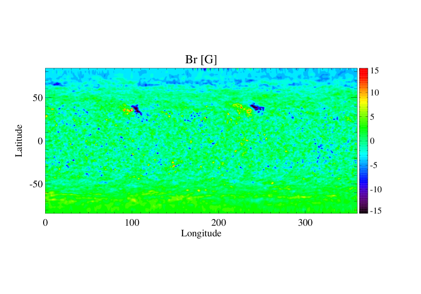
Figure 1: Synoptic magnetogram for Carrington Rotation 2077 obtained by GONG. The radial magnetic field at the photosphere is shown in the range $-15$ to $+15$ Gauss to show more detail. The color scale is saturated in the active regions where the largest and smallest values are $-45.4\,$G and $27.9\,$G.

We will use the GONG synoptic magnetogram for Carrington Rotation 2077 (CR2077, from November 20 to December 17, 2008) as an example to demonstrate the problem. The magnetogram contains the radial field on a $180\times 360$ latitude-longitude grid on the solar surface. The grid spacing is uniform in $\cos\theta$ (or sine of the latitude) and in longitude $\phi$. Figure 1 shows the radial field.

Section 2 discusses the naive and more sophisticated ways of obtaining the potential field solution with spherical harmonics. Section 3 describes an alternative approach using an iterative finite difference. The various methods are compared in the final Section 4, where we also demonstrate the ringing effect that can arise in the spherical harmonics solution, and we draw our conclusions.

2 Potential Field Solution Based on Spherical Harmonics

To turn the analytic prescription given in the introduction into a scheme that works with real magnetograms, one has to pick the maximum degree $N$, and evaluate the integrals in equation (10) for each pair of $n$ and $m$ up to the highest order. The resulting $f_{nm}$ coefficients can be used to construct the 3D potential magnetic field solution at any given point using equation (11).

2.1 Naive Spherical Harmonics Approach

The simplest approximation to equation (10) is a discrete integral using the original magnetogram data:

$$f_{nm}=\frac{1}{4\pi[n+(n+1)R^{2n+1}]}\sum_{i=1}^{N_{\theta}}\sum_{j=1}^{N_{\phi}}(\Delta\cos\theta)_{i}(\Delta\phi)_{j}M_{i,j}Y_{nm}(\theta_{i},\phi_{j})$$ (12)

where the $M_{i,j}$ is the radial field in a pixel of the $N_{\theta}$ by $N_{\phi}$ sized magnetogram. The pixel is centered at the $(\theta_{i},\phi_{j})$ coordinates, and the area of the pixel is given by $(\Delta\cos\theta)_{i}(\Delta\phi)_{j}$.

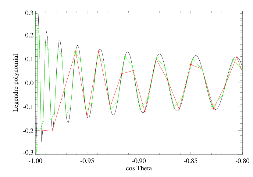
Figure 2: Discrete representations of the $P_{90,0}$ associated Legendre polynomial as a function of $\cos\theta$ near the “south pole” at $\cos\theta=-1$. The black curve shows an accurate representation with 1800 grid points uniformly distributed in the $[-1,1]$ range. The red curve represents the polynomial on 180 grid points uniform in $\cos\theta$, while the green curve uses 181 grid points that are uniformly distributed in $\theta$ including the poles at $\theta=0$ and $\theta=\pi$.

Unfortunately, the uniform $\cos\theta$ mesh used by most of the magnetograms is not at all optimal to evaluate the integral in equation (10). In fact this procedure will only work with maximum order $N$ that is much less than $N_{\theta}$. Figure 2 shows the $P_{90,0}$ associated Legendre polynomial discretized in different ways. The red curve shows the discretization on 180 grid points that are uniform in $\cos\theta$. Clearly the red curve is a very poor representation near the poles, where $\cos\theta=\pm 1$. This is important, because the amplitude of the Legendre polynomial is actually largest near the poles. This means that the orthonormal property is not satisfied in the discrete sense, and the coefficients obtained with equation (12) are very inaccurate. The Legendre polynomial can be represented much better on a uniform $\theta$ grid (shown by the green curve in Figure 2), as we will discuss below.

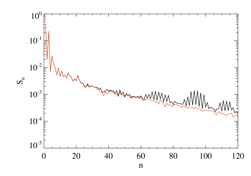
Figure 3: Power spectrum $S_{n}=\sum_{m}f^{2}_{nm}$ of the spherical harmonics expansion with the original (black line) and remeshed (red line) magnetograms.

A clear signal of this problem is that the amplitudes of the higher order spherical harmonics are not getting smaller with increasing indexes $n$ and $m$, i.e., the harmonic expansion is not converging. The black line in Figure 3 shows the amplitudes $S_{n}=\sum_{m}f^{2}_{nm}$ which is oscillating wildly for $n>60$ for this $360\times 180$ magnetogram. The oscillations are almost exclusively due to the $f_{n0}$ coefficients, the $m\neq 0$ coefficients are well behaved. This plot can be directly compared with Figure 15 in Altschuler et al. (1977), where the power spectrum is more-or-less exponentially decaying. We believe that the reason is that these authors used a least-square fitting to the line-of-sight (LOS) magnetic field instead of calculating the spherical harmonics from the radial field as shown above. While the two methods are identical analytically (assuming that the LOS and radial fields correspond to the same solution), the use of least-square fitting mitigates the lack of orthogonality among the discretized Legendre funtions, while the naive approach described above heavily relies on the orthogonality property.

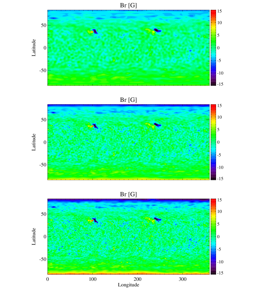
Figure 4: Comparison of the radial magnetic field at $r=1$ using the spherical harmonics expansion on the original magnetogram grid up to $N=60$ (top), $N=90$ (middle) and $N=120$ (bottom) order. These plots should be compared with the magnetogram shown in Figure 1. Note that the magnetic field in the polar regions is completely wrong for $N=90$ and $N=120$. The $N=60$ solution is reasonable, but the fine details are smoothed out.

Given the non-converging series expansion, the resulting potential field will be very inaccurate in the polar regions and will have essentially random values depending on the number of spherical harmonics used. This is demonstrated by Figure 4 that shows the radial magnetic field reconstructed with various number of harmonics using the original magnetogram grid. One would expect the radial component of the potential field to reproduce the magnetogram shown in Figure 1. Instead, we find that the solution deviates strongly in the polar region if the harmonics expansion is continued above $N=60$. For $N=60$ (or lower) the solution looks reasonable, but strongly smoothed due to the insufficient number of harmonics. This is most obvious around the active regions in the top panel of Figure 4.

We note that these numerical errors are not related or comparable to the observational uncertainties of the magnetograms, which are usually also quite large in the polar regions. The observational uncertainties are essentially unavoidable but are within some well-understood range. On the other hand, these numerical artifacts are definitely avoidable while the errors are essentialy unbounded if one uses too many harmonics.

2.2 Spherical Harmonics with Remeshed Magnetogram

One can get much more accurate results if the magnetogram is remeshed to a grid that is uniform in the co-latitude $\theta$, has an odd number of nodes, and contains the two poles $\theta=0$ and $\theta=\pi$. In fact this is the standard grid used in spherical harmonics transforms (e.g. Suda & Takami (2001)) and it is often referred to as using the Chebyshev nodes, since the uniform $\theta$ grid points correspond to the Chebyshev nodes in the original $\cos\theta$ coordinate which is the argument of the Legendre polynomials. Figure 2 shows that the Legendre polynomial is much better represented on the uniform $\theta$ grid than on the uniform $\cos\theta$ grid. Remeshing the magnetogram introduces some new adjustable parameters into the procedure: the number of grid cells $N^{\prime}_{\theta}$ on the new mesh, and the interpolation procedure.

If the remeshing is done with the same number of grid points as is in the original magnetogram grid, the latitudinal cell size at the equator will be a factor of $\pi/2$ larger than in the uniform-$\cos\theta$ grid. On the other hand, the uniform-$\theta$ grid will contain many more points than the original in the polar regions, so the interpolation procedure may create some unwanted artifacts. To maintain the resolution of the original data around the equator, we set $N^{\prime}_{\theta}$ to $(\pi/2)N_{\theta}$ rounded to an odd integer. For the remeshing we chose a simple linear interpolation procedure, and it works satisfactorily, but one could certainly use higher order interpolation procedures, such as splines. Before doing the interpolation, we add extra grid cells corresponding to the north and south poles of the magnetogram grid, and the values at these two extra cells are set as the average of the pixels around the poles:

$$M_{0} = \frac{1}{N_{\phi}}\sum_{j=1}^{N_{\phi}}M_{1,j}$$ (13)

$$M_{N_{\theta}+1} = \frac{1}{N_{\phi}}\sum_{j=1}^{N_{\phi}}M_{N_{\theta},j}$$ (14)

The co-latitude coordinates of the uniform-$\theta$ mesh are

$$\theta^{\prime}_{i^{\prime}}=\pi\frac{i^{\prime}-1}{N^{\prime}_{\theta}-1}$$ (15)

for $i^{\prime}=1\ldots N^{\prime}_{\theta}$. We use simple linear interpolation from the extended magnetogram mesh to the uniform $\theta$ mesh:

$$M^{\prime}_{i^{\prime},j}=\alpha M_{i,j}+(1-\alpha)M_{i^{\prime}+1,j}$$ (16)

where the $i$ index is determined so that $\theta_{i}\leq\theta^{\prime}_{i^{\prime}}\leq\theta_{i+1}$ and

$$\alpha=\frac{\theta_{i+1}-\theta^{\prime}_{i^{\prime}}}{\theta_{i+1}-\theta_{i}}$$ (17)

Finally the spherical harmonics coefficients are determined with the integral approximated as

$$f_{nm}=\frac{1}{4\pi[n+(n+1)R^{2n+1}]}\sum_{i=1}^{N^{\prime}_{\theta}}\sum_{j=1}^{N_{\phi}}\epsilon_{i}w_{i}(\Delta\phi)_{j}M^{\prime}_{i,j}Y_{nm}(\theta^{\prime}_{i},\phi_{j})$$ (18)

where $\epsilon_{1}=\epsilon_{N^{\prime}_{\theta}}=1/2$ and $\epsilon_{i}=1$ for all other indexes. The $w_{i}$ coefficients are the Clenshaw-Curtis weights (Clenshaw & Curtis, 1960; Potts, Steidl, & Tasche, 1998) defined as

$$w_{i}=\frac{1}{H}\sum_{k=0}^{H}\epsilon^{\prime}_{k}\frac{-2}{4k^{2}-1}\cos(2\pi k\theta^{\prime}_{i})$$ (19)

where $H=(N^{\prime}_{\theta}-1)/2$ and $\epsilon^{\prime}_{0}=\epsilon^{\prime}_{H}=1/2$ and $\epsilon^{\prime}_{k}=1$ for all other indexes. We note that for $N^{\prime}_{\theta}$ order of 10 or more

$$w_{i}\approx\frac{|\cos\theta^{\prime}_{i_{+}}-\cos\theta^{\prime}_{i_{-}}|}{2}$$ (20)

where $i_{+}=\min(i+1,N^{\prime}_{\theta})$ and $i_{-}=\max(i-1,1)$ are the indexes of the neighboring cells, or the cell itself at the poles.

Using the proper grid allows us to use larger number of spherical harmonics. $N$ is limited only by the $N\leq 2N^{\prime}_{\theta}/3$ and $N\leq N_{\phi}/3$ alias-free conditions (Suda & Takami, 2001). For our example $180\times 360$ magnetogram, we remesh it a to $283\times 360$ uniform-$\theta$ grid, and we can obtain accurate solutions up to $N=120$ degree spherical harmonics. Figure 5 shows the potential field solution obtained with the remeshed magnetogram grid with $N=120$. Compared with the naive method, the solution is much more reasonable in the polar regions. There is some smoothing when compared to the magnetogram shown in Figure 1, most obvious near the active regions.

While the remeshing is definitely a big improvement over using the original magnetogram, it would be nice to be able to use the original magnetogram data without remeshing and interpolation. The next section shows that this can be easily achieved with a finite difference solver.

3 Finite Difference Iterative Potential Field Solver (FDIPS)

The Laplace equation (1) with the boundary conditions (2) and (3) can be solved quite easily with an iterative finite difference method. The advantage of finite differences compared with spherical harmonics is that the boundary data given by the magnetogram directly effects the solution only locally, while the spherical harmonics are global functions, and their amplitudes depend on all of the magnetogram data. If the magnetogram contains large discontinuities, we expect the finite difference scheme to be better behaved.

The finite difference method has advantages if the solution is to be used in a finite difference code on the same grid, because one can guarantee zero divergence and curl for the magnetic field in the finite difference sense. The solution obtained with the spherical harmonics has zero divergence and curl analytically, but not on the finite difference grid, which may severly underresolve the high order spherical harmonic functions in some regions (see Figure 2).

The finite difference method was applied to the solar potential magnetic field problem as early as 1976 (Adams & Pneuman (1976)), but the method was limited by the computational resources available at the time. Solving a 3D Laplace equation on today’s computers is an almost trivial problem. We implemented the new Finite Difference Iterative Potential-field Solver (FDIPS) code in Fortran 90. The serial version does not require any external libraries, while the parallel version uses the Message Passing Interface (MPI) library for communication. FDIPS can solve the Laplace equation on a $150\times 180\times 360$ spherical grid to high accuracy on a single processor in less than an hour. The parallel code can solve the same problem in less than 5 minutes on 16 processors.

We briefly describe the algorithm in FDIPS. We use a staggered spherical grid: the magnetic field is discretized on cell faces while the potential is discretized at the cell centers. We use one layer of ghost cells to apply the boundary conditions so the cell centers are located at $r_{i},\theta_{j},\phi_{k}$ with $i=0\ldots N_{r}+1$, $j=0\ldots N_{\theta}+1$ and $k=0\ldots N_{\phi}+1$. The $\theta_{j}$ and $\phi_{k}$ coordinates of the real cells are given by the magnetogram, while the ghost cell coordinates are given by $\theta_{0}=-\theta_{1}$, $\theta_{N_{\theta}+1}=2\pi-\theta_{N_{\theta}}$, $\phi_{0}=\phi_{N_{\phi}}$, and $\phi_{N_{\phi}+1}=\phi_{1}$. We allow for a non-uniform radial grid extending from $r=1$ to $R$, but for sake of simplicity in this paper a uniform radial grid is used with $r_{i}=1+(i-1/2)\Delta r$ with $\Delta r=(R-r)/N_{r}$.

The radial magnetic field components are located at the radial cell interfaces at $(r_{i+1/2},\theta_{j},\phi_{k})$ where $r_{i+1/2}=(r_{i}+r_{i+1})/2$ for $i=0\ldots N_{r}$, $j=1\ldots N_{\theta}$ and $k=1\ldots N_{\phi}$. Similarly the latitudinal components are at $r_{i},\theta_{j+1/2},\phi_{k}$ with $\cos\theta_{j+1/2}=(\cos\theta_{j}+\cos\theta_{j+1})/2$, and $j=0\ldots N_{\theta}$. Note that the interface is taken half-way in the $\cos\theta$ coordinate and not in $\theta$, because this makes the cells equal area when the magnetogram is given on uniform $\cos\theta$ grid. Finally the longitudinal field components are located at $(r_{i},\theta_{j},\phi_{k+1/2})$ where $\phi_{k+1/2}=(\phi_{k}+\phi_{k+1})/2$ for $k=0\ldots N_{\phi}$.

The staggered discretization keeps the stencil of the Laplace operator compact and it makes the boundary condtions relatively simple. The magnetic field is obtained as a discrete gradient of $\Phi$:

$$B_{r,i+1/2,j,k} = \frac{\Phi_{i+1,j,k}-\Phi_{i,j,k}}{\Delta r}$$

$$B_{\theta,i,j+1/2,k} = \frac{\sin\theta_{j+1/2}(\Phi_{i,j+1,k}-\Phi_{i,j,k})}{r_{i}\Delta\cos\theta}$$

$$B_{\phi,i,j,k+1/2} = \frac{\Phi_{i,j,k+1}-\Phi_{i,j,k}}{r_{i}\sin\theta_{j}\Delta\phi}$$ (21)

Note the $\sin\theta/\Delta\cos\theta$ factor in the $\theta$ derivative for the uniform $\cos\theta$ grid. For uniform $\theta$ grid this is replaced with $1/\Delta\theta$. The divergence of the magnetic field, i.e. the Laplace of $\Phi$ is obtained as

$$0=(\nabla^{2}\Phi)_{i,j,k} = \frac{r^{2}_{i+1/2}B_{r,i+1/2,j,k}-r^{2}_{i-1/2,j,k}B_{r,i-1/2,j,k}}{r^{2}_{i}\Delta r}$$ (22)

$$+ \frac{\sin\theta_{j+1/2}B_{\theta,i,j+1/2,k}-\sin\theta_{j-1/2}B_{\theta,i,j-1/2,k}}{r_{i}\Delta\cos\theta}$$

$$+ \frac{B_{\phi,i,j,k+1/2}-B_{\phi,i,j,k-1/2}}{r_{i}\sin\theta_{j}\Delta\phi}$$

Again $1/\Delta\cos\theta$ is used for the uniform $\cos\theta$ grid, while on the uniform $\theta$ grid this is replaced with $1/(\sin\theta\Delta\theta)$.

The magnetogram boundary condition is applied by setting the inner ghost cell as

$$\Phi_{0,j,k}=\Phi_{1,j,k}-\Delta r\,M^{\prime}_{j,k}$$ (23)

where $M^{\prime}_{j,k}=M_{j,k}-\bar{M}$ is the magnetogram with the average field (i.e. the monopole due to observation errors)

$$\bar{M}=\frac{1}{4\pi}\sum_{j,k}(\Delta\cos\theta)_{j}(\Delta\phi)_{k}M_{j,k}$$ (24)

removed. The zero potential at $r_{N_{r}+1/2}=R$ is enforced by setting the ghost cell as

$$\Phi_{N_{r}+1,j,k}=-\Phi_{N_{r},j,k}$$ (25)

The boundary conditions at the poles are a bit tricky. Cells $(i,1,k)$ and $(i,1,k^{\prime})$ are on opposite sides of the north pole if $k^{\prime}=\textrm{mod}(k-1+N_{\phi}/2,N_{\phi})+1$. Therefore the ghost cells in the $\theta$ direction are set as $\Phi_{i,0,k}=\Phi_{i,1,k^{\prime}}$ and $\Phi_{i,N_{\theta}+1,k}=\Phi_{i,N_{\theta},k^{\prime}}$. We note here that $N_{\phi}$ is assumed to be an even number. The periodic boundaries in the $\phi$ direction are simple: $\Phi_{i,j,0}=\Phi_{i,j,N_{\phi}}$ and $\Phi_{i,j,N_{\phi}+1}=\Phi_{i,j,1}$.

We need to find $\Phi_{i,j,k}$ that satisfies the discrete Laplace equation (22) with the boundary conditions applied via the ghost cells. The initial guess is $\Phi=0$ which provides a non-zero residual because of the inhomogeneous boundary condition at the inner boundary applied by equation (23). We use this residual with a negative sign as the righ-hand-side of the Poisson equation $(\nabla^{2}\Phi)_{i,j,k}=R_{i,j,k}$, and use $\Phi_{0,j,k}=\Phi_{1,j,k}$ as the new homogeneous inner boundary condition instead of (23). We use the Krylov-type iterative method BiCGSTAB (van der Vorst, 1992) to find the solution. The linear system is preconditioned with an Incomplete Lower-Upper decomposition (ILU) preconditioner to speed up the convergence. We use ILU(0) with no fill-in compared to the original matrix structure, so the preconditioner is a diagonal matrix, but its elements depend on all elements of the original matrix. We have implemented a serial as well as a parallel version of the algorithm. In the parallel version the preconditioner is applied separately in each subdomain. FDIPS finds an accurate (down to $10^{-10}$ relative error) solution on a $180^{3}$ grid in less than 1000 iterations. Even running serially, this takes less than an hour on today’s computers.

Once the solution is found in terms of the discrete potential $\Phi_{i,j,k}$, we apply the original boundary conditions including (23) and calculate the magnetic field with equation(21). The divergence of the magnetic field will be zero to the accuracy of the Poisson solver. The curl of the magnetic field will be zero in a finite difference sense simply because it is constructed as the discrete gradient of the potential. The boundary condition at the inner boundary is also satisfied exactly: $B_{r,i=1/2,j,k}=M^{\prime}_{j,k}$. Averaging $rB_{\phi}$ and $rB_{\theta}$ to the $r_{N_{r}+1/2}=R$ position at the outer boundary also gives exactly zero tangential fields due to the equations (25) and (21). Depending on the application, we may interpolate the potential magnetic field onto a collocated grid, or use it on the original staggered grid.

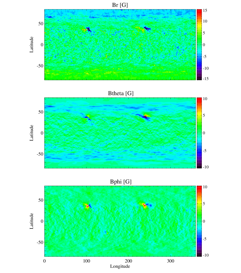
Figure 6: Magnetic field solution at $r=1$ using the finite difference code FDIPS on a $150\times 360\times 180$ grid. The radial component (top panel) agrees exactly with the magnetogram shown in Figure 1 except for the removal of the average field (the monopole). The tangential components (middle and bottom panels) agree well with the remeshed spherical harmonics solution shown in Figure 5.

Figure 6 shows the solution of the magnetic field obtained with the finite difference solver FDIPS on a $150\times 360\times 180$ grid. Since we use the same uniform-$\cos\theta$ grid as the magnetogram, the obtained radial field is identical with the magnetogram at $r=1$. The tangential components agree well with the remeshed spherical harmonics solution shown in Figure 5. It took 1166 iterations to get a solution with a relative accuracy of $10^{-10}$. The run time was almost exactly one hour on a 2.66 GHz Intel CPU.

4 Discussion and Conclusions

We have discussed various ways to obtain the potential field solution based on solar magnetograms. While spherical harmonics provide an efficient and elegant method, there are some subtle restrictions that require attention. If one wants to use many spherical harmonics (the same order as the number of magnetogram pixels in the colatitude direction), the magnetogram data on the $N_{\theta}\times N_{\phi}$ grid has to be remeshed onto a uniform-$\theta$ grid with $N^{\prime}_{\theta}\times N_{\phi}$ points, $N^{\prime}_{\theta}$ must be an odd number, and the new grid must include both poles. After the remeshing the maximum degree of harmonics $N$ is only limited by the anti-alias limit to $\min(2N^{\prime}_{\theta}/3$, $N_{\phi}/3)$. We used a simple linear interpolation for the remeshing.

The remeshing can be avoided by the use of a 3D finite difference scheme. One can use the original magnetogram grid, and the only freedom is in choosing the radial discretization. The finite difference scheme provides a solution that is fully compatible with the boundary conditions, and the solution has zero divergence and curl in the finite difference sense.

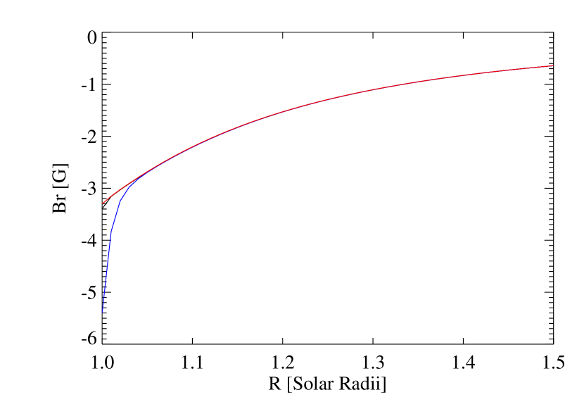
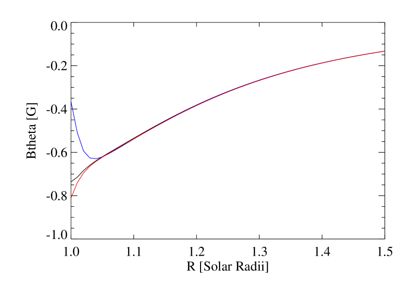
Figure 7: The radial and latitudinal components of the magnetic field along the radial coordinate at fixed $76.5\arcdeg$ latitude and $30\arcdeg$ longitude. The solutions are obtained with the naive (blue line) and remeshed (red line) harmonics approaches with $N=120$, as well as with finite differences (black line).

Figure 7 compares the solutions obtained with the three methods along the radial direction for a fixed latitude $\theta=76.5\arcdeg$ and longitude $\phi=30\arcdeg$. The spherical harmonics series were truncated at $N=120$ for both the naive and remeshed methods. The naive spherical harmonics algorithm gives incorrect results close to the solar surface where the high order harmonics dominate. This is most obvious for the radial component, which is given at $r=1$ by the magnetogram, and it is exactly reproduced by the finite difference scheme. The latitudinal component at $r=1$ is also very different from the values given by the remeshed harmonics and the finite differences. The latter two methods agree reasonably well with each other. For radial distances above $r=1.05$ all three methods agree quite well.

So far we restricted our example to a GONG magnetogram taken at the solar minimum. If one uses an MDI magnetogram during solar maximum, the largest magnetic fields are much stronger (order of 1000 G) and the resolution of the magnetogram is much finer (order of 1000 pixels). The finer magnetogram resolution allows going to larger number of harmonics, even when using the original magnetogram grid (naive approach). But the strong and sharp gradients in the magnetogram will bring out another problem with the spherical harmonics approach, the ringing effect. The ringing is due to the so-called Gibbs phenomenon: the step-function like magnetogram data results in high amplitude high order harmonics in Fourier space. The ringing effect and other artifacts are discussed in great detail by Tran (2009).

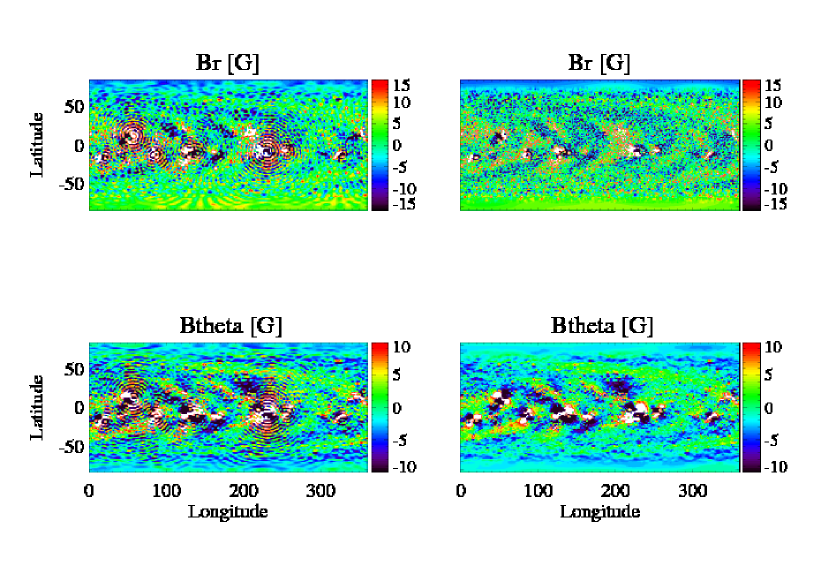
Figure 8: Radial and latitudinal components of the potential field solution at $r=1$ for the MDI magnetogram for CR2029 obtained with remeshed spherical harmonics algorithm with maximum order $N=90$ (left) and with FDIPS using a $150\times 360\times 180$ grid (right). The color scale is saturated in the active regions.

Figure 8 demonstrates this effect on the $3600\times 1080$ resolution MDI magnetogram for Carrington Rotation 2029 (from April 21 to May 18, 2005), with the maximum radial field strength around $\pm 3000\,$G. The remeshed harmonics method with $N=90$ is compared with the finite difference method on a $150\times 360\times 180$ grid (the magnetogram data is coarsened to a $360\times 180$ grid). In the spherical harmonics solution the ringing is very clearly visible around the active regions, both in the radial and latitudinal components. The finite difference scheme, on the other hand, shows no sign of ringing in either components. This is obvious for the radial component, which simply coincides with the coarsened magnetogram, but for the latitudinal component it is due to the fact that the finite difference solution of the Laplace equation does not suffer from ringing artifacts even for discontinuous boundary data. For the spherical harmonics approach the ringing becomes weaker with increased number of harmonics, but it is quite apparent even for $N=180$ (not shown). The results of the remeshed and naive harmonics methods are essentially the same up to $N=180$, i.e. the ringing is not due to the remeshing of the magnetogram.

In terms of computational efficiency, a good implementation of the spherical harmonics scheme is much faster than the finite difference scheme. In fact, it may be more costly to construct the potential field solution on a 3D grid from the spherical harmonics coefficients than obtaining the coefficients themselves. Our Fortran 90 code can obtain the spherical coefficients up to $N=60$, 90 and 120 degrees in 1, 1.8 and 3.3 seconds, respectively, while the reconstruction of the solution on the $151\times 361\times 180$ grid takes 5, 12, and 20 minutes, respectively. All timings were done on a single 2.66 GHz Intel CPU. The reconstruction cost can be improved by running the code in parallel, and/or truncating the series in parts of the grid where the higher order harmonics have a negligible contribution. We also note that going beyond about $N=360$ harmonics becomes fairly complicated (Potts, Steidl, & Tasche, 1998).

The computational cost of the finite difference scheme scales with the number of grid cells and the number of iterations. The number of iterations is fairly constant for multigrid type methods, but for the Krylov sub-space schemes it grows with the problem size, although slower than linearly. The finite difference scheme can be sped up by parallelizing the code, which is fairly straightforward for the Krylov subspace schemes. Since we limit the ILU preconditioning to operate independently on the subdomains of each processor, the preconditioner becomes less efficient as the number of processors increases, which results in an increase in the number of iterations. To minimize this effect, the parallel FDIPS code splits the grid in the $\theta$ and $\phi$ directions only, so the subdomains in each processor contain the full radial extent of the grid. Our experiments confirmed that using this domain decomposition, the number of iterations indeed does not depend much on the number of processors. Our largest test so far involves a $450\times 540\times 1200$ grid with 30 times more cells than the $150\times 180\times 360$ grids discussed in most of this paper. For the large problem we need about 8,500 iterations to reach the $10^{-10}$ relative accuracy, a factor of 9 increase relative to the smaller problem. Using 108 CPU-s, the solution is obtained in about 5.3 hours.

Despite the various limitations, for some applications the spherical harmonics approach may still be preferred. For example if the solution is needed to obtain a spherical power spectrum of the solar magnetic field. If the solution is to be used in a finite difference code, the finite difference solution is probably preferable. We are using the FDIPS code to generate the potential field solution as the initial field for our solar corona model (van der Holst et al., 2010).

This paper attempts to call the attention of astrophysicists and solar physicists to the limitations and potential pitfalls of using the spherical harmonics approach to obtain a potential field solution. The spherical harmonics representation of the potential field solutions are available from several synoptic magnetogram providers, although the details of the method used to obtain the spherical harmonics is not always clear. A spherical harmonics based PFSS package implemented in IDL is available as part of the Solar-Soft library (http://www.lmsal.com/solarsoft). This package uses the magnetogram remeshing technique either onto the Chebyshev (uniform-$\theta$) or the Legendre collocation points.

We are not aware of any publically available code that uses finite differences to solve this particular problem. To allow other researchers to use and compare the two approaches, we make our finite difference code FDIPS publically available at the http://csem.engin.umich.edu/fdips/ website.

Figure 5: Magnetic field solution at $r=1$ using the remeshed spherical harmonics up to $N=120$ degree. The radial compnents (top panel) well reproduces the magnetogram shown in Figure 1, although some of the details are slightly smoothed out.

References

- Schatten, Wilcox, & Ness (1969) Schatten, K. J., Wilcox, J. M. & Ness, N. F. 1969, Sol. Phys., 6, 442
- Altschuler et al. (1977) Altschuler, M. D., Levine, R. H., Stix, M., & Harvey, J. 1977, Sol. Phys., 51, 345
- Suda & Takami (2001) Suda, R. & Takami, M. 2001, Math. of Comp., 71, 703
- Clenshaw & Curtis (1960) Clenshaw, C. W. & Curtis, A. R. 1960, Numerishe Mathematik, 2, 197
- Potts, Steidl, & Tasche (1998) Potts, D., Steidl, G., & Tasche, M. 1998, Linear Algebra Appl., 275, 433
- Adams & Pneuman (1976) Adams, J. & Pneuman, G. W. 1976, Sol. Phys., 46, 185
- van der Vorst (1992) van der Vorst, H. 1992, SIAM J. Sci. Statist. Comput., 13, 631
- Tran (2009) Tran, T. 2009, “Improving the Predictions of Solar Wind Speed and Interplanetary Magnetic Field at the Earth”, Ph.D. thesis, UCLA
- van der Holst et al. (2010) van der Holst, B., Manchester IV, W. B., Frazin, R. A., Vásquez, A. M., Tóth, G., & Gombosi, T. I. 2010, ApJ, 725, 1373