A model for magnetically coupled sympathetic eruptions

Abstract

Sympathetic eruptions on the Sun have been observed for several decades, but the mechanisms by which one eruption can trigger another one remain poorly understood. We present a 3D MHD simulation that suggests two possible magnetic trigger mechanisms for sympathetic eruptions. We consider a configuration that contains two coronal flux ropes located within a pseudo-streamer and one rope located next to it. A sequence of eruptions is initiated by triggering the eruption of the flux rope next to the streamer. The expansion of the rope leads to two consecutive reconnection events, each of which triggers the eruption of a flux rope by removing a sufficient amount of overlying flux. The simulation qualitatively reproduces important aspects of the global sympathetic event on 2010 August 1 and provides a scenario for so-called twin filament eruptions. The suggested mechanisms are applicable also for sympathetic eruptions occurring in other magnetic configurations.

1. Introduction

Solar eruptions are observed as filament (or prominence) eruptions, flares, and coronal mass ejections (CMEs). It is now well established that these three phenomena are different observational manifestations of a single eruption, which is caused by the destabilization of a localized volume of the coronal magnetic field. The detailed mechanisms that trigger and drive eruptions are still under debate, and a large number of theoretical models have been developed (e.g., Forbes, 2010).

Virtually all existing models consider single eruptions. The Sun, however, also produces sympathetic eruptions, which occur within a relatively short period of time – either in one, typically complex, active region (e.g., Liu et al., 2009) or in different source regions, which occasionally cover a full hemisphere (so-called “global eruptions”; Zhukov & Veselovsky, 2007). It has been debated whether the close temporal correlation between sympathetic eruptions is purely coincidental, or whether they are causally linked (e.g., Biesecker & Thompson, 2000). Both statistical investigations (e.g., Moon et al., 2002; Wheatland & Craig, 2006) and detailed case studies (e.g., Wang et al., 2001) indicate that physical connections between them exist.

The exact nature of these connections has yet to be established. They have been attributed, for instance, to convective motions or destabilization by large-scale waves (e.g., Ramsey & Smith, 1966; Bumba & Klvana, 1993). At present, it seems most likely that the mechanisms by which one eruption can trigger another one act in the corona and are of a magnetic nature. Perturbations traveling along field lines that connect source regions of eruptions (e.g., Jiang et al., 2008) and changes in the background field due to reconnection (e.g., Ding et al., 2006; Zuccarello et al., 2009) have been considered. In an analysis of a global sympathetic event (see Section 2), Schrijver & Title (2011) found evidence for connections between all involved source regions via structural features like separators and quasi-separatrix layers (QSLs; Priest & Forbes, 1992; Démoulin et al., 1996); suggesting the importance of the structural properties of the large-scale coronal field in the genesis of sympathetic eruptions.

A magnetic configuration that appears to be prone to producing sympathetic eruptions is a unipolar streamer or pseudo-streamer (PS; e.g., Hundhausen, 1972; Wang et al., 2007). A PS is morphologically similar to a helmet streamer, but divides open fields of like polarity and contains an even number (typically two) of closed flux lobes below its cusp. PSs are quite common in the corona (e.g., Eselevich et al., 1999; Riley & Luhmann, 2011) and occasionally harbor two filaments. It seems that if one of these erupts, the other one follows shortly thereafter (so-called “twin filament eruptions”; Panasenco & Velli, 2010).

Here we present a numerical simulation that suggests two possible magnetic trigger mechanisms for sympathetic eruptions. It was inspired by the global sympathetic event on 2010 August 1, which involved a twin filament eruption in a PS.

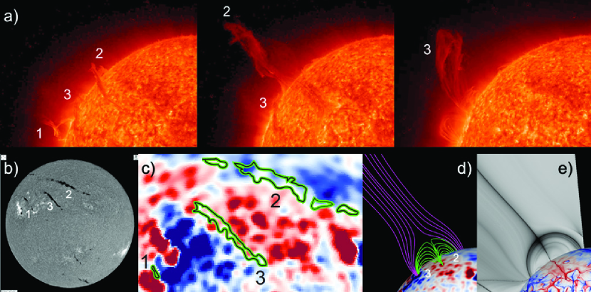
Figure 1.— (a:) STEREO-Ahead/EUVI 304 Å  observations of three subsequent prominence eruptions (marked by their order of eruption) on 2010 August 1, shown at 02:56, 09:16, and 22:06 UT (from left to right). (b): Big Bear Observatory H$\alpha$ observation on 2010 July 30, showing the corresponding pre-eruptive filaments. (c): Filament contours (drawn by eye) overlaid on a synoptic magnetogram for Carrington rotation 2099, with red (blue) showing positive (negative) radial fields. (d): Magnetic field lines from a corresponding PFSS extrapolation, revealing a pseudo-streamer. Green lines outline the lobes in which filaments 2 and 3 were located, pink lines show adjacent coronal holes. (e): Coronal distribution of $Q$ (grayscale) and photospheric distribution of slog $Q$, where red (blue) outlines positive (negative) magnetic fluxes.

2. The sympathetic eruptions on 2010 August 1

A detailed account of the individual eruptions that occurred in this global event can be found in Schrijver & Title (2011). Here we focus on a subset of three consecutive filament eruptions, all of which evolved into a separate CME. Figures 1a, b, and c show, respectively, the eruptions as seen by STEREO/EUVI (Howard et al., 2008), the pre-eruptive filaments, and a synoptic magnetogram obtained from SoHO/MDI (Scherrer et al., 1995) data. The large filaments 2 and 3 were located along the inversion lines dividing an elongated positive polarity and two bracketing negative polarities; the small filament 1 was located at the edge of the southern negative polarity. A potential field source surface extrapolation (PFSS; e.g., Schatten et al., 1969) for Carrington rotation 2099 reveals that filaments 2 and 3 were located in the lobes of a PS (Figure 1d; see also Panasenco & Velli 2010).

Figure 1e shows a cut through the coronal distribution of the squashing factor $Q$ (Titov et al., 2002) above filaments 2 and 3. The dark lines of high $Q$ outline structural features and exhibit here a shape characteristic for a PS (compare with Figure 3b below). The photospheric distribution shows slog $Q$ (Titov et al., 2011), depicting the footprints of (quasi-)separatrix surfaces. The structural skeleton of a PS consists of two separatrix surfaces, one vertical and one dome-like, which are both surrounded by a thin QSL (Masson et al., 2009) and intersect at a separator (Titov et al., 2011). It has been demonstrated that current sheet formation and reconnection occur preferably at such separators (e.g., Baum & Bratenahl, 1980; Lau & Finn, 1990).

The presence of the PS above filaments 2 and 3 suggests that the CME associated with filament eruption 1 may have triggered the subsequent eruptions by destabilizing the PS, presumably by inducing reconnection at its separator. We now describe an MHD simulation that enabled us to test this scenario using an idealized model.

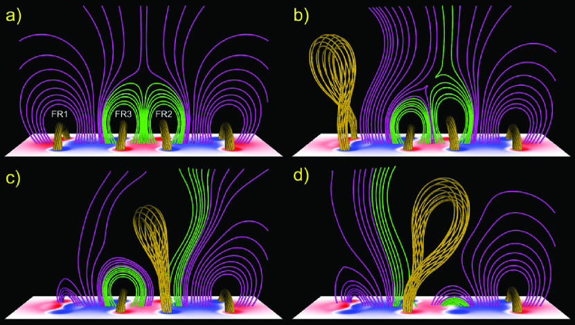
Figure 2.— Snapshots from the simulation, showing magnetic field lines with fixed footpoints and the normal component of the magnetic field at the bottom plane, where red (blue) depicts positive (negative) fields. Orange lines belong to the flux ropes, green ones to the initial pseudo-streamer lobes, and pink ones to initially closed or (semi-)open overlying flux. Panel (a) shows the configuration after initial relaxation and (b–d) show the successive flux rope eruptions and ambient field evolution at $t=85,126,\mathrm{and}\,181\,\tau_{a}$, respectively. “Already erupted” flux ropes are omitted for clarity. (An animation of this figure is available in the online journal.)

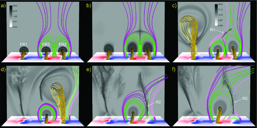
Figure 3.— Illustration of the two reconnection phases that trigger the successive flux rope eruptions in the pseudo-streamer. Field lines are colored as in Figure 2. The transparent inverted grayscale in the central plane, $\{y=0\}$, shows the logarithmic distribution of $|\mathbf{j}|/|\mathbf{B}|$, where $\mathbf{j}$ is the electric current density, outlining flux rope currents and thin current layers. Fainter field line segments are located behind the transparent layer. Panel (a) shows the initial configuration, (b) the system after relaxation, and (c–f) show the dynamic evolution, at $t=85,126,142,\mathrm{and}\,158\,\tau_{a}$, respectively. Panels (a,b) and (c–f) use a different scaling of $|\mathbf{j}|/|\mathbf{B}|$, respectively. Panel (c) shows reconnection R1, which triggers the eruption of FR2, and (e,f) show reconnection R2, which triggers the eruption of FR3. Panel (d) shows a state between the two reconnection phases. (An animation of this figure is available in the online journal.)

3. Numerical simulation

The basic simulation setup is as in Török et al. (2011), where two instances of the coronal flux rope model by Titov & Démoulin (1999, hereafter TD) were used to simulate the interaction of two flux ropes in a PS. Here we add a TD configuration on each side of the PS (Figure 2a). The new configuration on the left is used to model the CME associated with filament eruption 1, while the new one on the right is merely used to obtain a (line-)symmetric initial configuration, which facilitates the construction of a numerical equilibrium. It does not significantly participate in the dynamic evolution described below. The flux ropes FR1-3 are intended to model filaments 1-3.

We integrate the zero $\beta$ compressible ideal MHD equations, neglecting thermal pressure and gravity. The equations are normalized by the initial TD torus axis apex height, $R-d$ (see TD), the maximum initial magnetic field strength and Alfvén velocity, $\boldsymbol{B}_{0\mathrm{max}}$ and $v_{a0\mathrm{max}}$, and derived quantities. The Alfvén time is $\tau_{a}=(R-d)/v_{a0\mathrm{max}}$. We use a nonuniform cartesian grid of size $[-25,25]\times[-25,25]\times[0,50]$ with resolution $\simeq 0.04$ in the flux rope area. The initial density distribution is $\rho_{0}(\boldsymbol{x})=|\boldsymbol{B}_{0}\,(\boldsymbol{x})|^{3/2}$, such that $v_{a}(\boldsymbol{x})$ decreases slowly with distance from the flux concentrations. For further numerical details we refer to Török & Kliem (2003).

The model parameters are chosen such that all flux ropes are initially stable with respect to the helical kink (Török et al., 2004) and torus instabilities (TI; Kliem & Török, 2006). The ropes are placed along the $y$ direction, at $x=\pm 1.5\,\mathrm{and}\pm 5.5$, and have identical parameters ($R=2.75$, $a=0.8$, $d=1.75$, $L=0.5$, $q=4.64$; see TD). The signs of the sub-photospheric point charges, $\pm q$, are set according to the signs of the polarities surrounding filaments 1-3 (Figure 1c). The half-distance between the charges, $L$, is such that the TI can be triggered by a relatively weak perturbation (Schrijver et al., 2008). To obtain a numerically stable initial configuration that contains (semi-)open field above the PS lobes, the two charges associated with each flux rope are adjusted to $-0.55\,q/0.65\,q$ (for FR1 and FR4) and to $-0.34\,q/0.24\,q$ (for FR2 and FR3). The twist is chosen left-handed for all ropes to account for the observed dextral chirality of filaments 2 and 3 (Panasenco & Velli, 2010).

We first relax the system for $85\,\tau_{a}$ and reset time to zero. Then we trigger the eruption of FR1 by imposing localized converging flows at the bottom plane (as in Török et al. 2011), which slowly drive the polarities surrounding FR1 toward the local inversion line, yielding a quasi-static expansion of the rope’s ambient field. The flows are imposed for $25\,\tau_{a}$ (including phases of linear increase [decrease] to a maximum velocity of $0.02\,v_{a0\mathrm{max}}$ [to zero], each lasting $5\,\tau_{a}$).

Though we solve the ideal MHD equations, extra diffusion is introduced by numerical differencing (as in every MHD code that models solar magnetic fields). This numerical diffusion is localized in regions where the current density is largest, and leads to reconnection of magnetic field lines. Although it is much larger than the diffusion expected on the Sun, experience has shown that simulations produce solutions with physically expected behavior, as long as the numerical diffusion is sufficiently small. We therefore expect that our simulation indicates the true evolution of the system, but that the reconnection rates might differ from those present on the Sun.

4. Results

Figures 2 and 3 summarize the main dynamics and reconnection occurring in the simulation. Figure 3a shows the initial configuration and Figures 2a and 3b show the system after relaxation, during which weak current layers form at the PS separatrix surfaces, but no noticeable reconnection occurs. Note the correspondence between the current layer pattern and the $Q$-distribution shown in Figure 1e.

As the converging flows are applied, FR1 starts to rise slowly, in response to the quasi-static expansion of its ambient field. In contrast to other simulations, where such flows have been used to create a flux rope from a sheared arcade (e.g., Amari et al., 2000), they do not lead here to noticeable reconnection. The slow rise lasts until the rope reaches the critical height for TI onset at $t\approx 40\,\tau_{a}$, after which it rapidly accelerates upward driven by the instability (Török & Kliem, 2007; Fan & Gibson, 2007; Schrijver et al., 2008; Aulanier et al., 2010). FR1 attains a maximum velocity of $\approx 0.45\,v_{a0\mathrm{max}}$ at $t\approx 90\,\tau_{a}$ before it slowly decelerates. Figure 2b shows the system in the course of this eruption. The rise of the rope is slightly inclined, due to the asymmetry of its ambient field (e.g., Filippov et al., 2001). The rope rotates counterclockwise about its rise direction (as seen from above), due to the conversion of its twist into writhe (e.g., Green et al., 2007).

The expansion of FR1’s ambient field compresses the field between FR1 and the PS, particularly at larger heights where it is weak (see online animations). As a result, a tilted arc-shaped current layer forms around the PS separator (Figures 3c and 4). Further compression by the eruption steepens the current densities until reconnection (R1) between the open flux to the left of the PS and the closed flux in the right PS lobe sets in. The lobe flux then starts to open up, while the open flux starts to close down above the left PS lobe (Figures 2b and 3c). This successively decreases (increases) the magnetic tension above FR2 (FR3), so that FR2 rises slowly, while FR3 is slowly pushed downward. At $t\approx 95\,\tau_{a}$ FR2 reaches the critical height for TI onset and erupts, attaining a maximum velocity of $\approx 0.60\,v_{a0\mathrm{max}}$ at $t\approx 120\,\tau_{a}$. Figure 2c shows that FR2 also rises non-radially, but rotates less than FR1. The apparently smaller rotation of FR2 is due to the faster decay of its overlying field with height, which leads to a distribution of the total rotation over a larger height range than for FR1 (Török et al., 2010). By the time shown, FR1 has fully erupted, an elongated vertical current layer has formed in its wake (Figure 3d), and reconnection therein has produced cusp-shaped field lines below it. As FR2 erupts, it rapidly pushes the arc-shaped current layer to large heights (Figure 3d). While R1 still commences for some time, it does not play anymore a significant role for the following evolution.

A vertical current layer also forms below FR2. The subsequent reconnection (R2) initially involves the very same flux systems that took part in R1. The flux previously closed down by R1 opens up again, and the flux previously opened up by R1 – and by the expansion of FR2 – closes down to form cusp-shaped field lines below the current layer (Figure 3e). After these fluxes are exhausted, R2 continues, now involving the left PS lobe and the open flux to the right of the PS. While the former opens up, the latter closes down as part of the growing cusp (Figure 3f). Thus, R2 continuously removes closed flux above FR3. As before, this progressive weakening of magnetic tension leads to a slow rise of the rope, followed by its eruption (Figures 3f and 2d). The rapid acceleration of FR3 by the TI starts at $t\approx 138\,\tau_{a}$, yielding a maximum velocity of $\approx 0.35\,v_{a0\mathrm{max}}$ at $t\approx 175\,\tau_{a}$. The rope shows a significant rotation and an inclined rise which is now mainly directed toward the positive $x$ direction.

5. Discussion

The eruptions of FR2 and FR3 are initiated by the removal of a sufficient amount of stabilizing flux above the flux ropes via reconnection. R1 is similar to quadrupolar “breakthrough” or “breakout” reconnection (Syrovatskii, 1982; Antiochos et al., 1999). Here it is driven by a nearby CME rather than by an expanding arcade and, in contrast to the breakout model, a flux rope is present prior to eruption. R2, on the other hand, corresponds to standard flare reconnection in the wake of a CME. Here it removes flux from the adjacent PS lobe, thereby triggering the eruption of FR3. A similar mechanism for the initiation of a second eruption in a PS was suggested by Cheng et al. (2005), who, however, attributed it to reconnection inflows rather than to flux removal. We emphasize that R1 and R2 merely trigger the eruptions, which are driven by the TI and supported by the associated flare reconnection (e.g., Vršnak, 2008). Thus, in the system studied here, both PS eruptions require the presence of a pre-eruptive flux rope. We further note that the reconnections do not have to commence for the whole time period until the TI sets in. It is sufficient if they remove enough flux for the subsequently slowly rising flux ropes to reach the critical height for TI onset.

R1 is driven by a perturbation of limited duration – the lateral expansion of a nearby CME – and is slow since it involves only weak fields, around a separator at a significant height in the corona. Therefore, its success in triggering an eruption depends on parameters like the distance of the CME from the PS and the amount of pre-eruptive flux within the PS lobes. Indeed, if we sufficiently increase these parameters in the simulation we find that R1 still commences, but does not last long enough to trigger an eruption. In contrast, R2 is driven by the rise of FR2 and involves strong fields. It is therefore faster and more efficient, which supports the finding by Panasenco & Velli (2010) that an eruption in one lobe of a PS is often followed by an eruption in the neighboring lobe.

Figure  2 shows that the simulation correctly reproduces the order of the eruptions shown in Figure 1a and yields a good match of their inclinations and rotations. Assuming that the first eruption indeed triggered the subsequent ones, it is surprising that the filament located further away from it went off first. While filament 2 may simply have been closer to its stability limit than filament 3 (as indicated by its larger height; see Figure 1a), the simulation provides an alternative explanation: the perturbation of the separator yields an orientation of the current layer that leads to a removal of closed flux only in the right PS lobe (Figure 3c), thus enforcing the eruption of FR2. Hence, although we could not find observational signatures of R1 (presumably because the involved fields were too weak), the observed eruption sequence supports its occurrence. The time intervals between the simulated eruptions exhibit a ratio different to the observed ones. Matching the observed ratio requires a search for the appropriate model parameters and a more realistic modeling of reconnection, which are beyond the scope of this work.

FR2 reaches a velocity about 35 percent larger than FR1, which is in line with Liu (2007) and Fainshtein & Ivanov (2010), who found that CMEs associated with PSs are, on average, faster than those associated with helmet streamers. Liu (2007) suggested that this difference is due to the typically smaller amount of closed flux the former have to overcome. Indeed, FR1 has to pass through flux that is closed at all heights above it, while FR2 faces much less closed flux, a significant fraction of which is, moreover, removed by R1. FR3 remains significantly slower than FR2, most likely because it encounters more closed flux at eruption onset, and only partially opened flux later on (Figures 3e,f).

6. Conclusions

We present an MHD simulation of two successive flux rope eruptions in a PS, and we demonstrate how they can be triggered by a preceding nearby eruption. The simulation suggests a mechanism for twin filament eruptions and provides a scenario for a subset of the sympathetic eruptions on 2010 August 1. More realistic initial configurations and a more sophisticated treatment of reconnection are needed for a quantitative comparison with observations.

Our results support the conjecture that the trigger mechanisms of sympathetic eruptions can be related to the structural properties of the large-scale coronal field. However, while structural features are present in our model configuration, they do no connect the source region of the first eruption with the source regions of the subsequent ones. Moreover, the mere presence of such features in a source region is not a sufficient criterion for the occurrence of a sympathetic event, even if reconnection at structural features is triggered by a distant eruption. The conditions in the source region must be such that the resulting perturbation forces the region to cross the stability boundary.

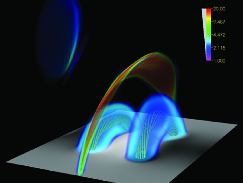
Figure 4.— Volume rendering of $|\mathbf{j}|/|\mathbf{B}|$ in the pseudo-streamer area at the same time as in Figures 2b and 3c, outlining the tilted arc-shaped current layer that forms around the separator.

The two trigger mechanisms presented here are independent and applicable also to other magnetic configurations. Triggering a sympathetic eruption by R1 requires the presence of a separator (or null point) above closed flux that stabilizes a pre-eruptive flux rope, which can be realized, in the simplest case, in a so-called “fan-spine” configuration (e.g., Antiochos, 1998; Pariat et al., 2009; Török et al., 2009). Triggering a sympathetic eruption by R2 requires the presence of an adjacent closed flux system overlying a flux rope, which can exist, for example, in quadrupolar configurations.

References

- Amari et al. (2000) Amari, T., Luciani, J. F., Mikic, Z., & Linker, J. 2000, ApJ, 529, L49
- Antiochos (1998) Antiochos, S. K. 1998, ApJ, 502, L181
- Antiochos et al. (1999) Antiochos, S. K., DeVore, C. R., & Klimchuk, J. A. 1999, ApJ, 510, 485
- Aulanier et al. (2010) Aulanier, G., Török, T., Démoulin, P., & DeLuca, E. E. 2010, ApJ, 708, 314
- Baum & Bratenahl (1980) Baum, P. J., & Bratenahl, A. 1980, Sol. Phys., 67, 245
- Biesecker & Thompson (2000) Biesecker, D. A., & Thompson, B. J. 2000, Journal of Atmospheric and Solar-Terrestrial Physics, 62, 1449
- Bumba & Klvana (1993) Bumba, V., & Klvana, M. 1993, Ap&SS, 199, 45
- Cheng et al. (2005) Cheng, J., Fang, C., Chen, P., & Ding, M. 2005, Chinese J. Astron. Astrophys., 5, 265
- Démoulin et al. (1996) Démoulin, P., Henoux, J. C., Priest, E. R., & Mandrini, C. H. 1996, A&A, 308, 643
- Ding et al. (2006) Ding, J. Y., Hu, Y. Q., & Wang, J. X. 2006, Sol. Phys., 235, 223
- Eselevich et al. (1999) Eselevich, V. G., Fainshtein, V. G., & Rudenko, G. V. 1999, Sol. Phys., 188, 277
- Fainshtein & Ivanov (2010) Fainshtein, V. G., & Ivanov, E. V. 2010, Sun and Geosphere, 5, 28
- Fan & Gibson (2007) Fan, Y., & Gibson, S. E. 2007, ApJ, 668, 1232
- Filippov et al. (2001) Filippov, B. P., Gopalswamy, N., & Lozhechkin, A. V. 2001, Sol. Phys., 203, 119
- Forbes (2010) Forbes, T. 2010, Models of coronal mass ejections and flares, ed. Schrijver, C. J. & Siscoe, G. L. (Cambridge University Press), 159–191
- Green et al. (2007) Green, L. M., Kliem, B., Török, T., van Driel-Gesztelyi, L., & Attrill, G. D. R. 2007, Sol. Phys., 246, 365
- Howard et al. (2008) Howard, R. A., Moses, J. D., Vourlidas, A., Newmark, J. S., Socker, D. G., Plunkett, S. P., Korendyke, C. M., Cook, J. W., Hurley, A., Davila, J. M., Thompson, W. T., St Cyr, O. C., Mentzell, E., Mehalick, K., Lemen, J. R., Wuelser, J. P., Duncan, D. W., Tarbell, T. D., Wolfson, C. J., Moore, A., Harrison, R. A., Waltham, N. R., Lang, J., Davis, C. J., Eyles, C. J., Mapson-Menard, H., Simnett, G. M., Halain, J. P., Defise, J. M., Mazy, E., Rochus, P., Mercier, R., Ravet, M. F., Delmotte, F., Auchere, F., Delaboudiniere, J. P., Bothmer, V., Deutsch, W., Wang, D., Rich, N., Cooper, S., Stephens, V., Maahs, G., Baugh, R., McMullin, D., & Carter, T. 2008, Space Sci. Rev., 136, 67
- Hundhausen (1972) Hundhausen, A. J. 1972, Coronal Expansion and Solar Wind, ed. Hundhausen, A. J.
- Jiang et al. (2008) Jiang, Y., Shen, Y., Yi, B., Yang, J., & Wang, J. 2008, ApJ, 677, 699
- Kliem & Török (2006) Kliem, B., & Török, T. 2006, Phys. Rev. Lett., 96, 255002
- Lau & Finn (1990) Lau, Y.-T., & Finn, J. M. 1990, ApJ, 350, 672
- Liu et al. (2009) Liu, C., Lee, J., Karlický, M., Prasad Choudhary, D., Deng, N., & Wang, H. 2009, ApJ, 703, 757
- Liu (2007) Liu, Y. 2007, ApJ, 654, L171
- Masson et al. (2009) Masson, S., Pariat, E., Aulanier, G., & Schrijver, C. J. 2009, ApJ, 700, 559
- Moon et al. (2002) Moon, Y., Choe, G. S., Park, Y. D., Wang, H., Gallagher, P. T., Chae, J., Yun, H. S., & Goode, P. R. 2002, ApJ, 574, 434
- Panasenco & Velli (2010) Panasenco, O., & Velli, M. M. 2010, AGU Fall Meeting Abstracts, A1663
- Pariat et al. (2009) Pariat, E., Antiochos, S. K., & DeVore, C. R. 2009, ApJ, 691, 61
- Priest & Forbes (1992) Priest, E. R., & Forbes, T. G. 1992, J. Geophys. Res., 97, 1521
- Ramsey & Smith (1966) Ramsey, H. E., & Smith, S. F. 1966, AJ, 71, 197
- Riley & Luhmann (2011) Riley, P., & Luhmann, J. G. 2011, Sol. Phys., under revision
- Schatten et al. (1969) Schatten, K. H., Wilcox, J. M., & Ness, N. F. 1969, Sol. Phys., 6, 442
- Scherrer et al. (1995) Scherrer, P. H., Bogart, R. S., Bush, R. I., Hoeksema, J. T., Kosovichev, A. G., Schou, J., Rosenberg, W., Springer, L., Tarbell, T. D., Title, A., Wolfson, C. J., Zayer, I., & MDI Engineering Team. 1995, Sol. Phys., 162, 129
- Schrijver et al. (2008) Schrijver, C. J., Elmore, C., Kliem, B., Török, T., & Title, A. M. 2008, ApJ, 674, 586
- Schrijver & Title (2011) Schrijver, C. J., & Title, A. M. 2011, Journal of Geophysical Research (Space Physics), 116, A04108
- Syrovatskii (1982) Syrovatskii, S. I. 1982, Sol. Phys., 76, 3
- Titov & Démoulin (1999) Titov, V. S., & Démoulin, P. 1999, A&A, 351, 707
- Titov et al. (2002) Titov, V. S., Hornig, G., & Démoulin, P. 2002, Journal of Geophysical Research (Space Physics), 107, 1164
- Titov et al. (2011) Titov, V. S., Mikić, Z., Linker, J. A., Lionello, R., & Antiochos, S. K. 2011, ApJ, 731, 111
- Török et al. (2009) Török, T., Aulanier, G., Schmieder, B., Reeves, K. K., & Golub, L. 2009, ApJ, 704, 485
- Török et al. (2010) Török, T., Berger, M. A., & Kliem, B. 2010, A&A, 516, A49
- Török et al. (2011) Török, T., Chandra, R., Pariat, E., Démoulin, P., Schmieder, B., Aulanier, G., Linton, M. G., & Mandrini, C. H. 2011, ApJ, 728, 65
- Török & Kliem (2003) Török, T., & Kliem, B. 2003, A&A, 406, 1043
- Török & Kliem (2007) —. 2007, Astron. Nachr., 328, 743
- Török et al. (2004) Török, T., Kliem, B., & Titov, V. S. 2004, A&A, 413, L27
- Vršnak (2008) Vršnak, B. 2008, Annales Geophysicae, 26, 3089
- Wang et al. (2001) Wang, H., Chae, J., Yurchyshyn, V., Yang, G., Steinegger, M., & Goode, P. 2001, ApJ, 559, 1171
- Wang et al. (2007) Wang, Y., Sheeley, Jr., N. R., & Rich, N. B. 2007, ApJ, 658, 1340
- Wheatland & Craig (2006) Wheatland, M. S., & Craig, I. J. D. 2006, Sol. Phys., 238, 73
- Zhukov & Veselovsky (2007) Zhukov, A. N., & Veselovsky, I. S. 2007, ApJ, 664, L131
- Zuccarello et al. (2009) Zuccarello, F., Romano, P., Farnik, F., Karlicky, M., Contarino, L., Battiato, V., Guglielmino, S. L., Comparato, M., & Ugarte-Urra, I. 2009, A&A, 493, 629