CHIANTI – an atomic database for emission lines - Paper XV: Version 9, improvements for the X-ray satellite lines

Abstract

CHIANTI contains a large quantity of atomic data for the analysis of astrophysical spectra. Programs are available in IDL and Python to perform calculation of the expected emergent spectrum from these sources. The database includes atomic energy levels, wavelengths, radiative transition probabilities, rate coefficients for collisional excitation, ionization, and recombination, as well as data to calculate free–free, free–bound, and two-photon continuum emission. In Version 9, we improve the modelling of the satellite lines at X-ray wavelengths by explicitly including autoionization and dielectronic recombination processes in the calculation of level populations for select members of the lithium isoelectronic sequence and Fe xviii–xxiii. In addition, existing datasets are updated, new ions added and new total recombination rates for several Fe ions are included. All data and IDL programs are freely available at http://www.chiantidatabase.org or through SolarSoft and the Python code ChiantiPy is also freely available at https://github.com/chianti-atomic/ChiantiPy.

1 Introduction

The goal of the CHIANTI atomic database for astrophysical spectroscopy is to provide the atomic parameters needed to analyze spectra from high-temperature, low-density, optically-thin sources. The main goal of Version 9 of CHIANTI is to improve the modelling of the satellite lines, by explicitly including autoionization and dielectronic recombination processes in the level populations equations for the ion. Previously a separate ion model (referred to as the "d" model) that included dielectronic capture, autoionization and radiative decay was used to calculate the resulting dielectronic emissivities and these were combined with the standard model. The new method establishes a framework to take into account density-dependent effects in the future for fully integrating level-resolved ionization and recombination processes into the CHIANTI atomic models. For the latest Version 9, we begin with the lithium isoelectronic sequence and a set of Fe ions (Fe XVIII–XXIV).

In addition, existing datasets are updated, new ions added and new total recombination rates for several Fe ions are included.

1.1 Goals and methods

The intensity of an individual line of an single ion is given by

$$I\,(i\to f)\,=\,\frac{h\nu}{4\pi}\,A(i\to f)\,N_{i}$$ (1)

where $h\nu$ is the energy of the emitted photon, $A(i\to f)$ is the radiative decay rate from initial level i to final level f, and $N_{i}$ is the population density of level i. If the energy $h\nu$ is given in erg, then the units of $I(i\to f)$ are in erg cm^-3 s^-1 sr^-1 for a single ion.

The $N_{i}$ are obtained by solving the equilibrium level balance equations, which model the atomic processes populating and de-populating the levels. The atomic parameters include radiative decay rates (or $A$-values), electron and proton collisional rate coefficients, autoionization rates, and level-resolved recombination rates from the next-higher ionization state. The primary goal of this paper is to describe our calculations of autoionization rates and dielectronic recombination rates and their roles in the CHIANTI database.

In Version 3 of CHIANTI (Dere et al., 2001), the dielectronic lines were accounted for by a model that assumed that dielectronic recombination took place only from the ground level of the higher ionization stage. These processes were modeled by the the dielectronic ions, such as fe_24d, and atomic data for these models were kept in special directories. The parameters were based on the calculated atomic parameters of Kato et al. (1997). These calculations included the $1s2snl$ and $1s2pnl$ levels with $n=2,3,4$ and 5 levels and the $n=6$ levels for Fe, Ca and S and $l\leq n$. The radiative data files contained the autoionization rates as simply a decay process.

In CHIANTI version 8 (Del Zanna et al., 2015) the atomic models for the lithium sequence ions were updated with the collision strengths of Liang & Badnell (2011), which were provided for transitions between all bound levels with a valence electron with $n\leq 5$ and core electron excitations up to $n=4$. The radiative recombination rates of Badnell (2006) were included for the bound levels of the lithium-like ions, through $n=8$.

For the new Version 9, our approach has been to include a more complete description of each ion, by adding the autoionizing levels to the bound levels. For the lithium sequence, this includes bound levels $1s^{2}nl$ ($2\leq n\leq 8$; $l\leq n-1$) and autoionizing levels $1s2snl$ and $1s2pnl$ ($2\leq n\leq 8$; $l\leq n-1$). More details for each sequence and on the method of calculation are given below. The version 9 ion file structure is still described by the usual CHIANTI files but with the addition of a new file .auto containing the autoionization rates for each level. For example, the lithium-like ion Fe XXIV now contains an additional file fe_24.auto containing the autoionization rates. The direct inner-shell excitation and the radiative values to the bound states have been added (whenever they were not present) to the existing rate files. Dielectronic recombination rates into the levels above the ionization potential have been calculated following Burgess (1964) or, equivalently, equation 15 of Badnell et al. (2003).

Once the new ion models are created, the dielectronic ion models such as fe_24d are removed from the database.

1.2 Atomic data for the improved models

New energy levels, radiative decay rates and autoionization rates have been calculated with the AUTOSTRUCTURE (AS) code (Badnell, 2011) for the present work. Unless otherwise stated, all new radiative decay and autoionization rates have been taken from these calculations. A drawback with AS lies in the accuracy of the calculated energy levels above the ionization potential (IP) since the autoionization and radiative rates depend on the transition energy. However, AS does include a mechanism, using a SHFTIC file to correct the energies produced by AS. The values used in the SHFTIC were determined from observed energies and wavelengths and the corrected energies, the A-values and autoionization rates for all of the levels were calculated by one of us (KPD). These values are stored in the .wgfa and .auto files.

Various sources for accurate level energies, particularly above the IP, exist. We have used the NIST (Kramida et al., 2015) energy levels based on observed spectral lines where available. Recently, Rudolph et al. (2013) have used an EBIT electron beam trap to measure the wavelengths of photo-excited levels of highly excited species of Fe XVIII through Fe XXV illuminated with a mono-energetic synchrotron beam. These measurements have been included for the ions we discuss in this paper. Yerokhin & Surzhykov (2012) report relativistic configuration interaction energy levels for the 1s2s², 1s2p² and 1s2s2p configurations of elements between argon and krypton. These have been preferably used for the theoretical levels of these configurations for the ions for which they are available.

The calculations of Safronova (Kato et al., 1997) are available for levels above the IP for n up to 5, and for n=6 for the ions Fe XXIV, Ca XVIII and S XVI. More recently, these calculations for the n = 2 and 3 levels have been improved by Goryaev et al. (2017) and these have been used to create the SHFTIC files. The calculations of Safronova and Goryaev et al. (2017) are both based on a Z-expansion method and provide wavelengths, rather than level energies. It has been necessary to use bound state energies largely based on the NIST (Kramida et al., 2015) energies to determine level energies from the Safronova and Goryaev et al. (2017) calculations. In the case of the lithium iso-electronic sequence, our approach in using the AS corrections in the SHFTIC file is to use the individual level corrections for the 1s2s², 1s2p² and 1s2s2p configurations and an average correction for each of the n = 3, 4 and 5 individual configurations. For these latter three configurations, the corrections do not vary significantly and so the n = 5 correction is then applied to the n = 6, 7 and 8 configurations.

For the ions in the lithium isoelectronic sequence it is only possible to autoionize to the ground level 1s² ${}^{1}S_{0}$ level of the helium-like ion. Similarly, it is only possible to recombine dielectronically by collisions with the helium-like ion in the same ground level. For other ions, a larger number of levels offer the possibility of autoionization and dielectronic recombination. For example, the beryllium-like ion can autoionize to the 1s²2s and 1s²2p levels of lithium-like ions. The lithium-like ion in these levels can also dielectronically recombine to the beryllium-like ions.

1.3 Software implementation of explicit autoionization and dielectronic recombination processes

The principal modification to the software was to include levels of the recombining ion in the calculation of the population of the recombined ion. In the low density approximation, only the lowest level of the recombining ion is populated and thus only one additional level is included in the solution for the level populations. For ions where dielectronic recombination/autionization proceed via a number of levels in the recombining ion, the software includes the population of all of the levels of the recombining ion. In this way, as the higher levels of the recombining ion become populated at finite densities, the dielectronic recombination can occur from these higher levels and alter the populations of the levels in the recombined ion giving rise to the satellite lines. This has been previously pointed out by e.g. Phillips et al. (1983), Jacobs et al. (1989) and Decaux et al. (2003). Details about the model are given in the Appendix.

2 New data for modeling autoionization and dielectronic recombination

2.1 The lithium isoelectronic sequence ions Zn xxviii, Ni xxvi, Fe xxiv, Cr xxii, Ti xx, Ca xviii, Ar xvi

The lithium sequence models of Version 8 have not been changed but they have been extended. In Version 8, the bound levels with principal quantum number n through 8 and levels above the IP with n up to 4 were included. Here, we extend the levels above the IP to n=8. The observed bound level energies are taken from the NIST database except where noted below. The energies for the $1s2l2l^{\prime}$ levels are derived from Yerokhin & Surzhykov (2012). For the $1s2l3l^{\prime}$ levels, the energies are derived from the calculations of Goryaev et al. (2017). For the $1s2lnl^{\prime}$ levels, the energies are derived from the calculations of Kato et al. (1997) for n=4 and 5 and for n=6 where available.

These energies are used to create the AS SHFTIC energy correction file for these ions. The corrections derived from the observed NIST energies and the energies of Yerokhin & Surzhykov (2012) are used directly. For the $1s2lnl^{\prime}$ levels where n = 3, 4, 5, or, 6, not all possible levels are provided by the calculations of Goryaev et al. (2017) or Kato et al. (1997). In these cases, average values of the corrections for each n level have been used. For values of n higher than covered by Kato et al. (1997), the average value for the highest n level available are used. For n = 4 and above, the corrections do not change very much with n.

2.1.1 Fe xxiv

Energies for levels below the ionization threshold are taken from Del Zanna (2006), and energies for several autoionizing levels were derived from the wavelengths given by Rudolph et al. (2013).

2.1.2 Ti xx

Wavelengths observed by Goldsmith et al. (1972) from the n = 3 levels have been used to extend the energy levels from the NIST database Kramida et al. (2015). Further, laboratory wavelengths measured by Fawcett & Ridgeley (1981) from the n = 4 levels have been included.

2.2 The lithium isoelectronic sequence ions S xiv, Si  xii, Al xi, Mg x, Ne viii, O vi, N v, and C iv

For these members of the lithium isoelectronic sequence, some observed energies for the bound levels are available from the the NIST database (Kramida et al., 2015). For the $1s2l2l^{\prime}$ and $1s2l3l^{\prime}$ levels, the energies are derived from the calculations of Goryaev et al. (2017). For the $1s2lnl^{\prime}$ levels, the energies are derived from the calculations of Kato et al. (1997) for n=4 and 5. For S xiv, Kato et al. (1997) also provide data for n=6.

As discussed above, the available data are used to create an optimized AS calculation of the energies, A-values and autoionization rates. These values are stored in the usual CHIANTI .elvlc, .wgfa and .auto files.

2.3 The beryllium isoelectronic sequence Fe xxiii

AS has been used to calculate the autoionization rates for transitions from the 1s2s²2p, 1s2s2p² and 1s2p³ states to the 1s²2s and 1s²2p states of Fe xxiv. As described above a SHFTIC correction file has been used. The corrections for the bound levels come from the NIST database (Kramida et al., 2015). The energies/wavelengths of Rudolph et al. (2013) have been used for the 1s2s²2p ³P₁ and the 1s2s²2p ¹P₁ levels and the corrections for the remaining 1s2s²2p and 1s2s2p² levels come from Yerokhin et al. (2017) and Rudolph et al. (2013). The previous version of CHIANTI included only the rates to the Fe xxv ground level of Palmeri et al. (2003).

2.4 The boron isoelectronic sequence Fe xxii

AS has been used to calculate the autoionization rates for transitions from the 1s2s²2p², 1s2s2p³ and 1s2p⁴ states to the 1s²2s²2p², 1s²2s2p³ and 1s²2p$4$ levels of Fe xxiii and have been used to create the fe_22.auto file. Again, the AS calculation of the energy levels involved a SHFTIC correction file. The corrections were based on the wavelengths of Rudolph et al. (2013). The wavelengths of Rudolph et al. (2013) have also been used for the 1s2s²2p^{2 2}D_3/2 and ²D_1/2 levels which are essentially degenerate in energy. In the previous version of CHIANTI, only the rates to the Fe xxiii ground level of Palmeri et al. (2003) were included.

2.5 The carbon isoelectronic sequence Fe xxi

Again, AS has been used to calculate the autoionization rates for transitions from 1s2s²2p³, 1s2s2p⁴ and 1s2p⁵ states the to the 1s²2s²2p, 1s²2s2p² and 1s²2p³ levels of Fe xxii to create the fe_21.auto file. The wavelengths of Rudolph et al. (2013) have been used for the 1s.2s²2p^{3 3}D₁ and ³S₁ levels of Fe xxii. In the previous version of CHIANTI, only the rates to the Fe xxii ground level of Palmeri et al. (2003) were included.

2.6 The nitrogen isoelectronic sequence Fe xx

For Fe xx, the 16 autoionizing levels included are in the 1s2s²2p⁴, 1s2s2p⁵ and 1s2p⁶ configurations. These levels can autoionize to the 20 levels of the 1s²2s²2p², 1s²2s2p³ 1s²2p⁴ configurations of Fe xxi. Observed wavelengths/energies of the autoionizing levels have been reported by Rudolph et al. (2013) for the 1s2s²2p^{4 4}P_5/2 and for 6 other levels of the 1s2s²2p⁴ configuration by Kramida et al. (2015). The remaining autoionizing levels have been optimized by using the average of the observed corrections to an unoptimized AS calculation.

2.7 The oxygen isoelectronic sequence Fe xix

For Fe xix, the 6 autoionizing levels included are in the 1s2s²2p⁵ and 1s2s2p⁶ configurations. These levels can autoionize to the 15 levels of the 1s²2s²2p³, 1s²2s2p⁴ 1s²2p⁵ configurations of Fe xx. The wavelengths of the transitions from the 1s2s²2p^{5 3}P₂ and ³P₁ levels to the ground have been measured by Rudolph et al. (2013). These associated energies have been used to optimize an AS calculation for both the 1s2s²2p⁵ and the 1s2s2p⁶ levels. For the latter, the correction for the optimized calculation has been assumed to be the same as the measured correction for the 1s2s²2p⁵ levels.

To summarize, the energies of the 1s2s²2p⁵ and 1s2s2p⁶ levels, the wavelengths associated with these levels and the autoionization values from these levels have been calculated with AS and updated in the CHIANTI fe_18.elvlc, fe_18.wgfa files and used to create the fe_18.auto files. Observed energies and wavelengths have been included and are given preference when used with the CHIANTI software.

2.8 The fluorine isoelectronic sequence Fe xviii

For Fe xviii we have calculated the autoionization rates from the single 1s2s²2p⁶ level using an optimized calculation of AS. The wavelength to the ground level has been measured by Rudolph et al. (2013) and the associated energy level has been used to optimize the AS calculation. Autoionization rates to the 1s²2s²2p⁴, 1s²2s2p⁵ and 1s2p⁶ levels of Fe xix have been included.

To summarize, the energy of the 1s2s²2p⁶ level and the wavelengths associated with this level have been updated in the CHIANTI fe_18.elvlc and fe_18.wgfa files, and the autoionization rates from this level have been placed in the new fe_18.auto file.

2.9 The sodium isoelectronic sequence: Al iii, Si iv, P v, S vi, Ar viii, K ix, Ca x, Cr xiv, Mn 15, Fe xvi and Ni xviii

In Version 8 (Del Zanna et al., 2015), new models of the sodium isoelectronc sequence were created. These models included 161 fine structure levels with 32 bound levels for 3s through 6h. Levels above the IP included the 2p⁵3s², 2p⁵3s3p, 2p⁵3s3d and 2p⁵3p3d configurations. The autoionization rates included in the Version 8 .wgfa files have been used to create the Version 9 .auto files.

2.10 A summary

To summarize, the optimized AS calculation has been used to provide the autoionization rates of the configurations mentioned above and have been used to determine the energies, A-values, and the autoionization rates included in the file of the recombined ion. These data have been incorporated into the energy level files .elvlc, the radiative data file .wgfa the autoionization file .auto. For the lithium-like ions and Fe xviii and Fe xxii an optimized AS calculation has been used to determine the theoretical energies of all the bound and auto-ionization levels and it observed levels and been inserted as well. For the remaining Fe ions Fe xxi, Fe xx, Fe xix, Fe xviii, the AS calculation has determined the theoretical values of the levels above the IP. The autoionization rates in the Version 8 radiative data files .wgfa have been removed for the ions mentioned above. For the sodium isoelectronic sequence, the Version 8 autoionization rates were transfered to a new Version 9 autoionization file .auto.

3 Autoionization and satellite lines

The spectra of helium-like ions and their satellites are strong features in astrophysical X-ray spectra. These features were first noted by Edlén & Tyrén (1939). Gabriel & Jordan (1969) suggested that the lines longward of the helium-like lines were due to transitions of the lithium-like lines, while Gabriel & Paget (1972) and Gabriel (1972) provided the rate equations for predicting the intensities of these lines and a naming convention for the lithium-like satellites.

Spectral lines created by radiative decays following dielectronic capture of free electrons into autoionizing levels play an important role in observed spectra, particularly in the X-ray wavelength region. The lithium sequence gives rise to many such lines as satellites to the helium sequence lines. Often these lines are blended with the helium sequence lines, which are important diagnostics of densities and temperatures, so their analysis requires an understanding of the lithium sequence blends. For example, Vainshtein & Safronova (1978) calculated the rates needed to predict the intensities for a large number of transitions from the n=2 satellites for nuclear charge Z of 3 to 34. Many of the n=2 lithium-like satellites are often as intense as some of the helium-like lines but many are also blended with each other and with the helium-like lines. The exact nature of the blending varies from element to element. For the case of the iron satellites, Bely-Dubau et al. (1979) performed calculations that showed that a large number of weaker satellites from the $n=3$ to $n=16$ lithium-like levels could produce significant blending as well. In addition, the lithium sequence dielectronic lines are useful for several spectroscopic diagnostic applications, e.g., to measure electron temperatures, departures from ionization equilibrium or thermal plasma. See, e.g., Gabriel (1972) and the reviews by Dubau & Volonte (1980), Phillips et al. (2008) and Del Zanna & Mason (2018). They have often been used in solar physics studies, and recently received significant attention by the astrophysics community, after the first high-resolution X-ray astrophysical spectra obtained by the Hitomi satellite, see e.g. Aharonian et al. (2018).

A particularly interesting diagnostic characteristic of some of the Fe satellite lines is that their intensities are sensitive to electron density. Phillips et al. (1983) showed that several satellite lines provide density diagnostics for densities above 10¹³ cm^-3. The density dependence is largely related to the density variation of the population of the metastable levels of the recombining ion which affects the populations of the recombined ion as a result of dielectronic recombination from levels above the ground level. This causes some satellite lines to be stronger and some to be weaker than in the case of a low density plasma. Jacobs et al. (1989) and Decaux et al. (2003) have carried out a similar study for temperature and densities consistent with solar flare plasmas, magnetically-confined laboratory plasmas and laser-produced plasmas.

3.1 Comparison with observations: BCS flare spectra of Fe XXV and Fe XXIV, Fe XXIII and Fe XXII

The Bent Crystal Spectrometer (BCS) (BCS; Acton et al., 1980; Culhane et al., 1981) experiment aboard the Solar Maximum Mission recorded X-ray spectra of numerous flares that produced significant Fe xxv and Fe xxiv emission that can be used to compare against synthetic spectra from CHIANTI Version 9. Recently, Rapley et al. (2017) have pointed out some problems with the BCS data. The main effect of the problem is that the dispersion tends to gradually increase with time during a solar flare. This is mainly seen in the Ca spectra and occasionally in the Fe spectra. However, this effect is quite obvious and it is possible to avoid using spectra where this occurs. Here we have used data from the decay phase of the 1989 April 1 flare near 07:32 UT that do not appear to have the problems described by Rapley et al. (2017).

Synthetic CHIANTI spectra have been calculated at a temperature of 2.12 $\times$ 10⁷ K and are plotted in Fig. 1 together with the BCS spectra. A pseudo-voigt profile, available in ChiantiPy, has been used to approximate the experimental line profile. The lines of Fe xxv, aside from the resonance line r, have been noted in green and the lines of Fe xxiv have been noted in red following the naming scheme of Gabriel & Paget (1972). The temperature was chosen to give the best agreement between the Fe xxiv satellite lines and the Fe xxv resonance line. The predicted lines of Fe xxiii between 1.87 and 1.88 Å are considerably weaker than observed, suggesting there is plasma at lower temperatures that is not accounted for by the isothermal model.

As a further example we show in Figures 2 and 3 SMM BCS spectra (black) of the 1980 Nov 5 flare during the peak phase, as observed in the Fe XXV and Ca XIX channels, compared with CHIANTI v.8 and v.9 isothermal spectra, calculated with the IDL codes. As it can be seen, the differences between v.9 and v.8 spectra are not large. Note that the wavelength scale of the BCS Fe XXV channel towards the longer wavelengths (Fe XXII) is not linear, as also pointed out by Rapley et al. (2017).

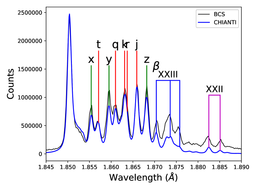
Figure 1: The BCS spectra (black) of the 1989 April 1 flare during the decay phase compared with the CHIANTI 9 spectrum (blue) for a temperature of 2.12 $\times$ 10⁷ K. Lines of Fe xxv and Fe xxiv are denoted with green and red vertical lines, respectively. Lines of Fe xxii and Fe xxiii are also indicated.

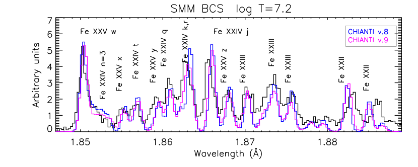
Figure 2: The SMM BCS spectra (black) of the 1980 Nov 5 flare during the peak phase, as observed in the Fe XXV channel, compared with CHIANTI v.8 and v. 9 isothermal spectra.

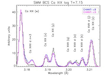
Figure 3: The BCS spectra (black) of the 1980 Nov 5 flare during the peak phase, as observed in the Ca XIX channel, compared with CHIANTI v.8 and v. 9 isothermal spectra.

4 Ionization and recombination rates

The fits to the dielectronic recombination rate coefficients of Fe viii through Fe xi have been replaced. Schmidt et al. (2008) used a combination of experimental measurements and theoretical calculations to provide the rate coefficients for Fe viii forming Fe vii and Fe ix forming Fe viii. Using a similar approach, Lestinsky et al. (2012) provide rate coefficients for Fe x forming Fe ix and Fe xi forming Fe x. The experimental measurements provide accurate values for the energies of the recombining ions above the IP. Using these energies, the rate coefficients were calculated with AS. The measurements for energies just above the IP are especially important for computing the rate coefficients at temperatures below 10⁴ K. The table of equilibrium ionization fractions (distributed as the file chianti.ioneq in the database) has been recomputed for Version 9. The ionization equilibria for the Fe ions vii through xii are shown in Figure 4 with values from the current version 9 and for the previous version 8.0.7. The largest change is for Fe viii, for which the ion fraction is up to 30% larger in CHIANTI 9.

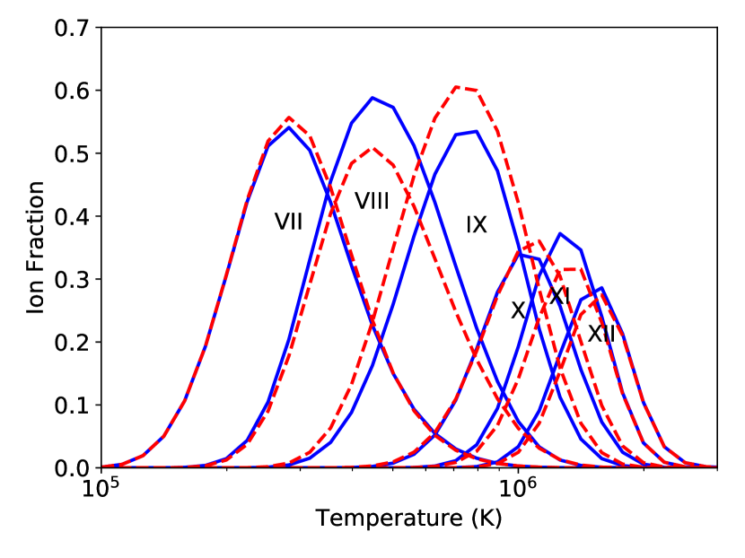
Figure 4: The ionization equilibria of Fe ions VII through XII, as calculated with the current CHIANTI Version 9 rates (blue), compared to the values in version 8.0.7 (dashed red)

5 Other updated ion datasets

5.1 N I

A mistake in the A-values for neutral nitrogen has been fixed. The nearly degenerate ${}^{2}D_{3/2,5/2}$ levels of the ground configuration 2s² 2p³ were erroneously inverted.

5.2 C II

The experimental energy for the $2s^{2}2p$ ${}^{2}P_{3/2}$ level was updated to the value of Cooksy et al. (1986), and the energies of the three $2s2p^{2}$ ${}^{4}P_{J}$ levels were updated to the values of Young et al. (2011).

5.3 Mn X

The Mn x model was added to CHIANTI 7 (Landi et al., 2012) and featured 48 fine structure levels. All of the 38 levels of the $3s^{2}3p^{3}3d$ configuration were assigned theoretical energies. Observed energies are now available from NIST for eight of the levels. These have been added to the energy level file and the wavelength file has been updated. No other changes to the model were performed.

5.4 Ca XIV

The excitation data in CHIANTI v.8 were from Landi & Bhatia (2005), and were calculated under the distorted wave (DW) approximation. It is well known that this approximation works very well for strong dipole-allowed transition, but typically underestimates the excitation of the forbidden lines, especially within the ground configuration. This was confirmed by a recent $R$-matrix calculation by Dong et al. (2012), where the excitation rate for the 943.58 Å forbidden transition is about a factor of two higher with the Dong et al. calculations. We have adopted the Dong et al. excitation rates, and supplemented them with A values from the recent GRASP2K calculations by Wang et al. (2016). The ratio of the forbidden line, often observed by SoHO SUMER, with the strongest line, the resonance EUV line at 193.87 Å observed with Hinode EIS, is about factor of 1.7 higher with the new model ion. This change brings into agreement SUMER and EIS observations, as shown in Parenti et al. (2017).

5.5 Fe X

In the analysis of the spectrum of Fe x by Del Zanna et al. (2012), level 25 (3s² 3p⁴ 3d ²D_3/2) was not assigned an observed energy or wavelength. However, the NIST database (Kramida et al., 2015) assigns an observed energy of 511 800 cm^-1 to this level and this has been inserted into the fe_10.elvlc file for Version 9 and the wavelengths of the lines decaying from this level have been recalculated.

5.6 Fe XII

Energies of six levels in the Fe xii model have been changed following the work of Wang et al. (2018). The observed energies of levels 21, 38, 84 and 87 have been modified; the observed energy assigned to level 85 has been removed; and an observed energy has been assigned to level 50. No other changes to the Fe xii model have been performed.

5.7 Fe XVIII

A modification was made to the fe_18.reclvl file. The 1–91 transition was found to have an anomalously high value at the highest tabulated temperature that was traced to the original data-set of Gu (2003). The value was replaced with one extrapolated from the lower temperature points.

The effective collision strengths for the bound levels were not correctly extrapolated above 7 MK when they were processed for CHIANTI 6 (Dere et al., 2009), and so the data have been re-processed for CHIANTI 9.

5.8 Fe XIX

A modification was made to the fe_19.reclvl file. The 1–160 transition was found to have an anomalously high value at the highest tabulated temperature that was traced to the original data-set of Gu (2003). The value was replaced with one extrapolated from the lower temperature points.

5.9 Fe XXI

A modification was made to the fe_21.reclvl file. The 1–179 transition was found to jump by four orders of magnitude between two adjacent temperatures, suggesting an error in the rates for this transition. Since the calculated rates were small, the transition has been removed from the file. The 1–215 transition was found to have an anomalously high value at the highest tabulated temperature and this value has been replaced with one extrapolated from the lower temperature points. Both of these problems were present in the original data-set of Gu (2003).

6 New ions: K IV

The CHIANTI model consists of the 5 fine structure levels in the ground configuration. Observed energies have been taken from version 5.3 of the NIST database (Kramida et al., 2015). Theoretical energies were taken from the calculations of Froese Fischer et al. (2006). The set of A-values come from Biémont & Hansen (1989)

The atomic data for K iv is rather sparse. The collision strengths have been taken from calculations of Galavis et al. (1995). They provide fine-structure collisions strengths among the ³P level but only LS collision strengths to the ¹D and ¹S levels in the ground configuration. For these latter levels, fine-structure collision strengths have been developed from these calculations by scaling the collision strengths according to the the statistical weight of the ³P levels.

7 Further additions to the CHIANTI IDL programs

7.1 CHIANTI_DEM

By default, the CHIANTI_DEM program was using the subroutine xrt_dem_iterative2.pro (Weber et al., 2004). This routine, widely used in solar physics and available within SolarSoft, is based on the robust chi-square fitting program mpfit.pro. Within this subroutine, the differential emission measure (DEM) is modelled assuming a spline, with a fixed selection of the nodes. As it turns out, the $DEM$ solutions are quite sensitive to the choice of nodes, so we have replaced the xrt_dem_iterative2.pro routine with a new subroutine, called MPFIT_DEM, where we allow for the definition of the number and location of the spline nodes. We also simplified substantially the code and introduced the option to input minimum and maximum limits to the spline values, which are passed to mpfit.pro. These limits are useful when a spectral line intensity is not measured but an upper limit can be defined. Various other options are available, as described in the header of the programs. The usage of the CHIANTI_DEM program is unchanged.

7.2 AIA temperature responses

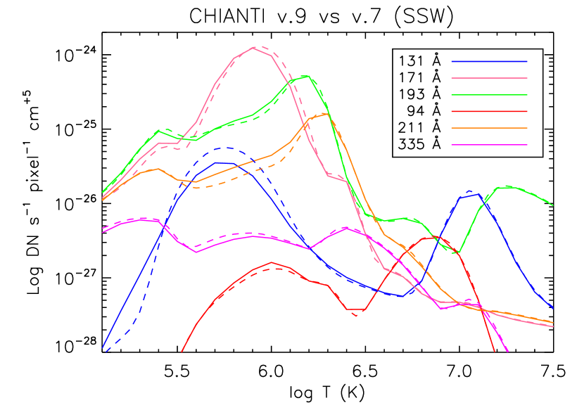
Figure 5: The AIA temperature responses as calculated with the CHIANTI Version 9 ionization equilibrium and atomic data (full lines), compared to the default AIA responses available within SolarSoft (dashed lines), which were calculated with CHIANTI v.7.

Upon suggestion of the SDO AIA PI (Dr. M. Cheung), we have now added a simple IDL program so that users can calculate the AIA temperature responses using the latest understanding of the decrease in the efficiency of the various broad-band filters, and the latest CHIANTI data. Users can also calculate the responses using different parameters (e.g., densities, chemical abundances) to see how they affect them. Figure 5 shows the AIA temperature responses as calculated with the CHIANTI Version 9 ionization equilibrium and atomic data, compared to the default AIA responses available within SolarSoft, which were calculated with CHIANTI v.7. The parameters (chemical abundances and constant pressure) are the same for both. The differences in the 131 and 171 Å channel responses mainly arise due to the changes in the ionization fractions of Fe viii and Fe ix (Sect. 4). The other differences are mainly due to updates of the ion data-sets. Note that the responses are calculated in the 25–900 Å wavelength region, and there are some significant off-band contributions above 400 Å, which were introduced in 2013 within the AIA programs.

8 Conclusions

We have improved the modelling of the satellite lines in at X-ray wavelengths with the explicit inclusion of autoionization and dielectronic recombination processes in the calculation of level populations. The changes, compared to the previous CHIANTI versions, are not large, which shows that the approximate treatment of the satellite lines was relatively accurate. The explicit inclusion of these rates provides a framework for further investigations of these processes at higher densities. Considering the further improvement in the wavelengths of the satellite lines, we believe that the present version can reliably be used for any astrophysical applications involving the satellite lines.

All data and IDL programs are freely available online and through the SolarSoft IDL library. ChiantiPy, the Python application for CHIANTI, is also freely available through Github.

Appendix A Implementation of the new collisional-radiative method within the IDL software

The main processes that form the doubly excited (autoionizing) states $s$ are inner-shell excitation of one electron in the lower ionization stage $Z^{+r}$, and the dielectronic capture (DC) of a free electron by the higher (ionization stage) ion $Z^{r+1}$ in the state $k$. The lower ion $Z^{+r}$ in the autoionizing state $s$ can then autoionize (releasing a free electron) to any of the states $k$ of the ion $Z^{r+1}$, or produce a radiative transition into any bound state $f$ of the recombined ion. The intensity of the satellite line, resulting from the decay to a final bound level $f$ of the lower ion $Z^{+r}$, is

$$I_{sf}=N_{s}A_{sf}$$ (A1)

where $A_{sf}$ is the radiative decay rate from level $s$ to the final level $f$, and $N_{s}$ is the population of the autoionizing state.

In previous versions of CHIANTI, and for the ions without autoionizing states, the level populations $p$ are obtained by solving the rate equations:

$$(A+N_{\rm e}\,(C^{e}+C^{p})+P)\,p=b\;,$$ (A2)

where $b$ is a vector set to zeros except for the first element which is 1. The most important matrices are those for the spontaneous decay processes ($A$), and for the collisional excitation/de-excitation due to electron impact ($C^{e}$). Additional matrices for photo-excitation ($P$) and proton excitation ($C^{p}$) and their de-excitation processes are also included.

The population of the autoionizing state due to dielectronic capture involves the solution of rate equations where both the recombined and recombining ions are included. Thus, in CHIANTI V.9 we have modified the IDL codes in order to solve for the level populations of all the levels of the lower (recombined) and higher (recombining) ion simultaneously. In order to do this, we have extended the matrices $A,C^{e},C^{p}$ and $P$ to include all the levels of the lower ion (including the autoionizing levels) and the bound levels of the higher ion. This means that the rates connecting the bound levels within each of the ions are included in the same way as in the previous versions, but we now have included the rates for the autoionizing levels and those connecting the two ions. This framework naturally takes into account density effects on the satellite lines related to the populations of the metastable levels in the recombining ions.

The population of the autoionizing state due to inner-shell excitation is calculated in a similar way as for the bound levels, including the inner-shell impact excitation rate $N_{\rm e}\,C^{e}_{is}$ in the rate equation. The rate coefficient $C^{e}_{is}$ is retrieved from the scaled effective collision strengths stored in the .scups file. The de-excitation rate due to a collision by a free electron is included as in the case of the bound levels, but this term is usually negligible.

The decay rate due to autoionization, $A^{\rm auto}_{sk}$, of the doubly-excited state $s$ to the state $k$ is included in the same way as the matrix $A$. The autoionization rates are stored in the .auto file. Note that in the case of the satellites of He-like ions, all autoionizations go to the ground state, where most of the population is. For the recombining ions with metastable levels, dielectronic capture from populated levels can occur and thus it is included, together with autoionization rates to those levels.

Dielectronic capture is effectively a population process for the autoionizing states $s$, proportional to the free electron density $N_{\rm e}$ and the population $N_{\rm k}$ of the recombining ion in its state $k$ involved in the capture. We have therefore included this populating process between states $k$ and $s$ as in the matrix $C^{e}$ of collisional excitation. The rate coefficient $C^{\rm dc}_{ks}$ for the capture of the free electron by the ion $Z^{r+1}$ in the state $k$ into a doubly-excited state $s$ of the lower ion $Z^{+r}$ is obtained from the autoionization rate applying the principle of detailed balance (e.g. Phillips et al. (2008)):

$$C^{\rm dc}_{ks}=\frac{h^{3}}{(2\pi mkT)^{3/2}}\frac{g_{s}}{2g_{k}}A^{\rm auto}_{sk}\exp\left(-\frac{E_{s}-E_{k}}{kT}\right)$$ (A3)

This is valid as long as the electrons have a Maxwellian distribution. To relate the populations of the lower and higher ions we also need to include ionization and recombination rates. We recall that currently CHIANTI includes collisional ionization (CI) rates between the ground states of the ions calculated by Dere (2007), and total radiative recombination (RR) and dielectronic recombination (DR) rates, also between the ground states of the ions. The recombination rates are mainly those calculated by N.R.Badnell and colleagues. The total DR rates from the ground state of the recombining ion were obtained by Badnell by summing up the contributions of all the autoionizing states. The total DR rate needs a correction, to avoid double counting the DR rates. As we have now included autoionizing levels in the model, for consistency we need to calculate the total DR due to the levels included in the model and originating from the ground level of the higher ion, and subtract this quantity from the total DR rate. The remaining rate is added in the matrix as a term connecting the two ground states.

The calculation of the total DR rate due to the autoionizing levels included in the model is not trivial, as in principle each autoionizing state could decay to another autoionizing level, as well as decay to a bound level $f^{\prime}$ of the recombined ion, or autoionize to a level of the recombining ion. We neglect the first process for two reasons. First, we note that the other two are the main ones, although we note that in some cases we do have some autoionizing levels that mainly decay to other autoionizing levels. The second reason is that the total DR rates have been calculated neglecting this cascading process. The total rate is therefore calculated as

$$c\;\sum_{s}\sum_{k}\frac{g_{s}}{2g_{k}}\;A^{\rm auto}_{sk}\;e^{-\frac{E_{s}-E_{k}}{kT}}\;\frac{\sum_{f^{\prime}<s}A_{sf^{\prime}}}{\sum_{k}A^{auto}_{sk}+\sum_{f^{\prime}<s}A_{sf^{\prime}}}$$ (A4)

where the constant $c=h^{3}\;(2\pi mkT)^{-3/2}$

The CI rates are included as they are available in CHIANTI, i.e., connecting the ground states. The RR rates are now included in two different ways. For most ions, the total RR rates from the ground state of the recombining ion are included in the matrix to connect to the ground state of the recombined ion.

For some ions, we have now introduced the level-resolved RR rates as calculated by N. Badnell. They are included with a new file, with the extension .rrlvl, with a format similar to that of the previous .reclvl files. We have included these level-resolved rates into the matrix. They typically increase the populations of the lower levels by 10% or so, but for higher levels can be the only populating process. To avoid double counting, as in the case of the DR rates, we sum the total RR of the level-resolved rates and subtract this value from the total RR. Any residual total RR is added as a rate connecting the two ground states.

Contributions to level populations due to cascades from bound levels is therefore now naturally included in the model ions, although for many ions most of the RR occurs into high-lying levels that are not currently included in the model. For many ions we have therefore retained the corrections due to these cascading effects as in the previous CHIANTI versions. Prior to CHIANTI 9 the radiative recombination rates were implemented as a post-processing step once the level population equations of the standard CHIANTI model had been solved, as described in Landi et al. (2006). These RR rates are stored in the .reclvl files. For the important Fe xvii–xxiii ions, the rates are from the calculation of Gu (2003) and the rate into a level includes both the direct radiative recombination rate and the indirect recombinations that come from cascading from higher levels, including the autoionization levels populated by dielectronic capture. The effects of these rates on the level populations is approximated with a correction, after the matrix is inverted, as in previous CHIANTI versions.

Note that a model CHIANTI ion can only have either direct level-resolved RR rates as in the .rrlvl files or the level-resolved RR including cascades as in the .reclvl files. Also note that the .reclvl files can only have recombination from the ground state, while the .rrlvl files can in principle include recombination from excited states. Finally, note that the CHIANTI programs assume that all the rates in these two files are on the same temperature grid, although the files in principle could have different temperature grids for each transitions.

After the matrices are populated and the populations obtained, we then normalise the populations of the lower ion so the total is one, as in the case of ions without autoionizing states. Note that the relative population of the two ions as obtained solving the two-ion rate equations can sometimes be different than what is obtained by assuming that the ion populations are all in the ground state (which is what is used in CHIANTI to calculate the relative ion charge state distributions). However, this effect is small and is not considered in this version 9.

Finally, we note that the new v.9 IDL codes are compatible with earlier CHIANTI v.8 data files, but the earlier CHIANTI v.8 IDL programs should not be used with the new v.9 format files.

References

- Acton et al. (1980) Acton, L. W., Finch, M. L., Gilbreth, C. W., et al. 1980, Sol. Phys., 65, 53
- Aharonian et al. (2018) Aharonian, F., Akamatsu, H., Akimoto, F., et al. 2018, Publications of the Astronomical Society of Japan, 70, 12
- Badnell (2006) Badnell, N. R. 2006, ApJS, 167, 334
- Badnell (2011) —. 2011, Computer Physics Communications, 182, 1528
- Badnell et al. (2003) Badnell, N. R., O’Mullane, M. G., Summers, H. P., et al. 2003, A&A, 406, 1151
- Bely-Dubau et al. (1979) Bely-Dubau, F., Gabriel, A. H., & Volonte, S. 1979, MNRAS, 189, 801
- Biémont & Hansen (1989) Biémont, E., & Hansen, J. E. 1989, Phys. Scr, 39, 308
- Burgess (1964) Burgess, A. 1964, ApJ, 139, 776
- Cooksy et al. (1986) Cooksy, A. L., Saykally, R. J., Brown, J. M., & Evenson, K. M. 1986, ApJ, 309, 828
- Culhane et al. (1981) Culhane, J. L., Rapley, C. G., Bentley, R. D., et al. 1981, ApJ, 244, L141
- Decaux et al. (2003) Decaux, V., Jacobs, V. L., Beiersdorfer, P., Liedahl, D. A., & Kahn, S. M. 2003, Physical Review A, 68, 012509
- Del Zanna (2006) Del Zanna, G. 2006, A&A, 447, 761
- Del Zanna et al. (2015) Del Zanna, G., Dere, K. P., Young, P. R., Landi, E., & Mason, H. E. 2015, A&A, 582, A56
- Del Zanna & Mason (2018) Del Zanna, G., & Mason, H. E. 2018, Living Reviews in Solar Physics, in press
- Del Zanna et al. (2012) Del Zanna, G., Storey, P. J., Badnell, N. R., & Mason, H. E. 2012, A&A, 541, A90
- Dere (2007) Dere, K. P. 2007, A&A, 466, 771
- Dere et al. (2001) Dere, K. P., Landi, E., Young, P. R., & Del Zanna, G. 2001, ApJS, 134, 331
- Dere et al. (2009) Dere, K. P., Landi, E., Young, P. R., et al. 2009, A&A, 498, 915
- Dong et al. (2012) Dong, F., Wang, F., Zhong, J., Liang, G., & Zhao, G. 2012, PASJ, 64, 131
- Dubau & Volonte (1980) Dubau, J., & Volonte, S. 1980, Reports on Progress in Physics, 43, 199
- Edlén & Tyrén (1939) Edlén, B., & Tyrén, F. 1939, Nature, 143, 940
- Fawcett & Ridgeley (1981) Fawcett, B. C., & Ridgeley, A. 1981, Journal of Physics B Atomic Molecular Physics, 14, 203
- Froese Fischer et al. (2006) Froese Fischer, C., Tachiev, G., & Irimia, A. 2006, Atomic Data and Nuclear Data Tables, 92, 607
- Gabriel (1972) Gabriel, A. H. 1972, MNRAS, 160, 99
- Gabriel & Jordan (1969) Gabriel, A. H., & Jordan, C. 1969, Nature, 221, 947
- Gabriel & Paget (1972) Gabriel, A. H., & Paget, T. M. 1972, Journal of Physics B Atomic Molecular Physics, 5, 673
- Galavis et al. (1995) Galavis, M. E., Mendoza, C., & Zeippen, C. J. 1995, Astronomy and Astrophysics Supplement Series, 111, 347
- Goldsmith et al. (1972) Goldsmith, S., Feldman, U., Oren, L., & Cohen, L. 1972, ApJ, 174, 209
- Goryaev et al. (2017) Goryaev, F. F., Vainshtein, L. A., & Urnov, A. M. 2017, Atomic Data and Nuclear Data Tables, 113, 117
- Gu (2003) Gu, M. F. 2003, ApJ, 582, 1241
- Hunter (2007) Hunter, J. D. 2007, Computing In Science & Engineering, 9, 90
- Jacobs et al. (1989) Jacobs, V. L., Doschek, G. A., Seely, J. F., & Cowan, R. D. 1989, Physical Review A, 39, 2411
- Jones et al. (2001–) Jones, E., Oliphant, T., Peterson, P., et al. 2001–, SciPy: Open source scientific tools for Python, scipy.org, [Online; accessed <today>]. http://www.scipy.org/
- Kato et al. (1997) Kato, T., Safronova, U., Shlypteseva, A., et al. 1997, Atomic Data and Nuclear Data Tables, 67, 225
- Kramida et al. (2015) Kramida, A., Yu. Ralchenko, Reader, J., & and NIST ASD Team. 2015, NIST Atomic Spectra Database (ver. 5.3), [Online]. Available: http://physics.nist.gov/asd [2017, August 23]. National Institute of Standards and Technology, Gaithersburg, MD.
- Landi & Bhatia (2005) Landi, E., & Bhatia, A. K. 2005, Atomic Data and Nuclear Data Tables, 90, 177
- Landi et al. (2012) Landi, E., Del Zanna, G., Young, P. R., Dere, K. P., & Mason, H. E. 2012, ApJ, 744, 99
- Landi et al. (2006) Landi, E., Del Zanna, G., Young, P. R., et al. 2006, ApJS, 162, 261
- Lestinsky et al. (2012) Lestinsky, M., Badnell, N. R., Bernhardt, D., et al. 2012, ApJ, 758, 40
- Liang & Badnell (2011) Liang, G. Y., & Badnell, N. R. 2011, A&A, 528, A69
- Palmeri et al. (2003) Palmeri, P., Mendoza, C., Kallman, T. R., & Bautista, M. A. 2003, A&A, 403, 1175
- Parenti et al. (2017) Parenti, S., del Zanna, G., Petralia, A., et al. 2017, ApJ, 846, 25
- Phillips et al. (2008) Phillips, K. J. H., Feldman, U., & Landi, E. 2008, Ultraviolet and X-ray Spectroscopy of the Solar Atmosphere (Published by Cambridge University Press, Cambridge, UK, 2008.)
- Phillips et al. (1983) Phillips, K. J. H., Lemen, J. R., Cowan, R. D., Doschek, G. A., & Leibacher, J. W. 1983, ApJ, 265, 1120
- Rapley et al. (2017) Rapley, C. G., Sylwester, J., & Phillips, K. J. H. 2017, Sol. Phys., 292, 50
- Rudolph et al. (2013) Rudolph, J. K., Bernitt, S., Epp, S. W., et al. 2013, Physical Review Letters, 111, 103002
- Schmidt et al. (2008) Schmidt, E. W., Schippers, S., Bernhardt, D., et al. 2008, A&A, 492, 265
- Vainshtein & Safronova (1978) Vainshtein, L. A., & Safronova, U. I. 1978, Atomic Data and Nuclear Data Tables, 21, 49
- van der Walt et al. (2011) van der Walt, S., Colbert, S. C., & Varoquaux, G. 2011, Computing in Science and Engineering, 13, 22
- Wang et al. (2018) Wang, K., Jönsson, P., Gaigalas, G., et al. 2018, ApJS, 235, 27
- Wang et al. (2016) Wang, K., Si, R., Dang, W., et al. 2016, ApJS, 223, 3
- Weber et al. (2004) Weber, M. A., Deluca, E. E., Golub, L., & Sette, A. L. 2004, in Multi-Wavelength Investigations of Solar Activity, ed. A. V. Stepanov, E. E. Benevolenskaya, & A. G. Kosovichev, Vol. 223, 321–328
- Yerokhin & Surzhykov (2012) Yerokhin, V. A., & Surzhykov, A. 2012, Phys. Rev. A, 86, 042507
- Yerokhin et al. (2017) Yerokhin, V. A., Surzhykov, A., & Müller, A. 2017, Phys. Rev. A, 96, 042505
- Young et al. (2011) Young, P. R., Feldman, U., & Lobel, A. 2011, ApJS, 196, 23