ALFVÉN WAVE SOLAR MODEL (AWSOM): CORONAL HEATING

Abstract

We present a new version of the Alfvén Wave Solar Model (AWSoM), a global model from the upper chromosphere to the corona and the heliosphere. The coronal heating and solar wind acceleration are addressed with low-frequency Alfvén wave turbulence. The injection of Alfvén wave energy at the inner boundary is such that the Poynting flux is proportional to the magnetic field strength. The three-dimensional magnetic field topology is simulated using data from photospheric magnetic field measurements. This model does not impose open-closed magnetic field boundaries; those develop self-consistently. The physics includes: (1) The model employs three different temperatures, namely the isotropic electron temperature and the parallel and perpendicular ion temperatures. The firehose, mirror, and ion-cyclotron instabilities due to the developing ion temperature anisotropy are accounted for. (2) The Alfvén waves are partially reflected by the Alfvén speed gradient and the vorticity along the field lines. The resulting counter-propagating waves are responsible for the nonlinear turbulent cascade. The balanced turbulence due to uncorrelated waves near the apex of the closed field lines and the resulting elevated temperatures are addressed. (3) To apportion the wave dissipation to the three temperatures, we employ the results of the theories of linear wave damping and nonlinear stochastic heating. (4) We have incorporated the collisional and collisionless electron heat conduction. We compare the simulated multi-wavelength EUV images of CR2107 with the observations from STEREO/EUVI and SDO/AIA instruments. We demonstrate that the reflection due to strong magnetic fields in proximity of active regions intensifies the dissipation and observable emission sufficiently.

1 INTRODUCTION

During the last few decades, considerable progress has been made in the understanding of the solar atmosphere due to the increased availability of observational data and the development of analytical and numerical models of the solar wind. One aspect of this development is the construction of complex three-dimensional (3D) models. These models can be validated with observations and further refined to improve the comparison. Important in the further progress of these models is a better understanding of the coronal heating and solar wind acceleration problem. Improvements in the theories of the coronal heating scenarios may result in more realistic models that are more reliable in predicting the solar wind conditions. Eventually, this may further improve the numerical forecasting of space weather events.

Recent Hinode observations suggested that there is more than enough energy in the chromospheric magnetic field fluctuations, which propagate away from the Sun, to heat the solar corona and maintain the temperatures at $1\;$MK (De Pontieu et al., 2007). With the Solar Dynamics Observatory (SDO) these waves were shown to be ubiquitously present in the transition region and low corona (McIntosh et al., 2011). These observations suggest that it is therefore appealing to develop a 3D solar corona and inner heliosphere model that is based on Alfvén wave turbulence and check if such a theoretical model reproduces emission features seen in the extreme ultraviolet (EUV) images. In our previous corona model (Sokolov et al., 2013), we demonstrated that Alfvén wave turbulence can indeed capture the overall observable EUV emission, with the exception of some of the details such as the emission around active regions.

There is a long history of Alfvén wave turbulence in the solar wind that dates back to the pioneering work of Coleman (1968), who concluded that turbulence is important in the solar wind near $1\;$AU based on Mariner 2 measurements. The earliest solar wind models that incorporated Alfvén wave turbulence were presented in Belcher & Davis (1971) and Alazraki & Couturier (1971), followed by 2D global corona models by Usmanov et al. (2000) and Hu et al. (2003). Suzuki & Inutsuka (2006) constructed a self-consistent 1D Alfvén wave turbulence model from the photosphere to inner heliosphere that included wave reflection and mode conversion from Alfvén to slow waves. This model was generalized to 2D by Matsumoto & Suzuki (2012) to account for turbulent cascade. Alfvén waves that propagate outward from the Sun are partially reflected by gradients due to stratification, which produces waves propagating in opposite directions, see for instance (Heinemann & Olbert, 1980; Leroy, 1980; Mattheus et al., 1999; Dmitruk et al., 2002; Verdini & Velli, 2007; Cranmer, 2010; Chandran et al., 2011). Counter-propagating waves are essential for the classical incompressible cascade (Velli et al., 1989) and hence the coronal heating. The reflection due to strong magnetic field gradients may be important in close proximity of the active regions, further intensifying the dissipation and the observable EUV emission. In the present paper, we will determine if this enhanced wave reflection does improve our model comparison with the observed EUV images.

Remote observations from the Ultraviolet Coronagraph Spectrometer (UVCS) have shown that the perpendicular ion temperature is much larger than the parallel ion temperature in the corona holes (Kohl et al., 1998; Li et al., 1998). Similarly, Helios observations have shown that the ion temperature in the inner heliosphere is anisotropic as well (Marsch et al., 1982). Several models have been constructed that take the ion temperature anisotropy into account, see for instance Leer & Axford (1972); Isenberg (1984); Fichtner & Fahr (1991); Chandran et al. (2011) for 1D analysis and Vásquez et al. (2003); Li et al. (2004) for 2D analysis. The ion temperature anisotropy has, to the best of our knowledge, not yet been incorporated in a 3D solar wind model.

In recent years, our solar wind efforts in the Space Weather Modeling Framework (SWMF, Tóth et al. (2012)) were focused on creating an Alfvén wave turbulence-driven solar corona and inner heliosphere model with a two-temperature approach for the electrons and ions. Our goal is to develop a single validated model that can produce realistic synthesized line-of-sight (LOS) images in the multi-wavelength EUV, and accurate $1\;$AU prediction of the solar wind properties. This model will also produce realistic background solar wind for simulations of coronal mass ejections (CMEs). van der Holst et al. (2010) constructed a solar wind model that has an inner boundary in the $1\;$MK corona and has separate electron and ion temperatures. It incorporated the collisional electron heat conduction and Alfvén wave transport and dissipation along the open field lines. This model was validated in Jin et al. (2012), while Evans et al. (2012) enhanced the model by including surface Alfvén waves. The two-temperature approach is important in producing a correct CME shock, otherwise a strong and unphysical heat precursor can appear ahead of the CME due to the heat conduction (Manchester et al., 2012; Jin et al., 2013). Meanwhile, Downs et al. (2010) developed a lower corona model that was able to reproduce synthesized EUV images, but for the coronal heating the model did still rely on ad hoc coronal heating functions. Sokolov et al. (2013) combined the aforementioned efforts into a single two-temperature model with Alfvén wave turbulence by incorporating the concept of balanced turbulence at the apex of the closed field lines, and via a concise analysis, the model was able to numerically resolve the upper chromosphere and transition region. This model was able to reproduce the overall morphology of coronal holes and active regions in the EUV images. Landi et al. (2013b) demonstrated that it was also able to capture the charge state evolution, while Oran et al. (2013) compared the model output to in-situ Ulysses observations.

Lionello et al. (2009) demonstrated that a 3D magnetohydrodynamic (MHD) lower corona model based on a combination of ad hoc coronal heating functions and with heat conduction was able to well reproduce many features in the observed EUV images. Odstrcil et al. (2005) showed that the ENLIL inner heliosphere MHD model prescribed by the empirical Wang–Sheeley–Arge (WSA) model (Arge & Pizzo, 2000) was able to capture the $1\;$AU observations, while Cohen et al. (2007); Feng et al. (2010); van der Holst et al. (2010) used the WSA to prescribe the coupled corona and inner inner heliosphere simulations to obtain $1\;$AU results.

In the approach taken in the Alfvén wave solar model (AWSoM) described in the current paper, we no longer rely on ad hoc heating functions. The physics incorporated into the AWSoM model allows us to produce realistic LOS images and $1\;$AU solar wind predictions in one single model. We present the theoretical approach and results in two companion papers. The present paper is the first one and describes the coronal heating methodology and electron heat conduction and presents the resulting synthesized images of the multi-wavelength EUV emission. We also demonstrate the newly implemented low dissipation MP5 limiter (Suresh & Huynh, 1997) in the BATS-R-US model. The reduced numerical dissipation allows us to clearly resolve the fine details in the solution, and allow a better comparison with observations. Our second paper, X. Meng et al. (in preparation), describes the impact of these changes on the solar wind acceleration and the $1\;$AU comparisons.

The outline of the paper is as follows: In Section 2, we present details of the theoretical model and discuss the numerical implementation. We first describe in Section 2.1 the Alfvén wave turbulence approach for the two-temperature model. In Section 2.2 we provide the derivation of the Alfvén wave propagation, reflection, and dissipation. In Section 2.3, we generalize this model to three temperatures by using anisotropic ion temperatures and the isotropic electron temperature. The implementation is described in Section 2.4. In Section 3, we demonstrate the performance of this model for Carrington rotation (CR) 2107 by comparing EUV images with observations. We conclude in Section 4 and provide details of the derivations in the appendices.

2 COMPUTATIONAL MODEL

We now present the equations of the AWSoM model. We first describe the two-temperature MHD equations for the electrons and ions to demonstrate the incorporation of the Alfvén wave turbulence and collisionless heat conduction. The details of the derivation of the Alfvén wave equations are presented in Section 2.2. In Section 2.3, these equations are generalized to ion temperature anisotropy. In Section 2.4, we give some details of the numerical implementation. We finalize this section with a discussion on the boundary conditions (Section 2.4.1).

2.1 Governing Equations of Two-temperature Model

The starting point of our model is the MHD equations, which well describe the large-scale, low-frequency phenomena of the solar corona and inner heliosphere plasma. In the inertial frame, the mass conservation, momentum conservation, and induction equation are

$$\frac{\partial\rho}{\partial t}+\nabla\cdot(\rho{\bf u})=0,$$ (1)

$$\frac{\partial(\rho{\bf u})}{\partial t}+\nabla\cdot\left(\rho{\bf u}{\bf u}-\frac{{\bf B}{\bf B}}{\mu_{0}}\right)+\nabla\left(P_{i}+P_{e}+\frac{B^{2}}{2\mu_{0}}+P_{A}\right)=-\rho\frac{GM_{\sun}}{r^{3}}{\bf r},$$ (2)

$$\frac{\partial{\bf B}}{\partial t}-\nabla\times({\bf u}\times{\bf B})=0,$$ (3)

respectively. In addition, the initial conditions should satisfy $\nabla\cdot{\bf B}=0$. The notation in these equations is as follows: $\rho$ is the mass density, ${\bf u}$ is the velocity, assumed to be the same for the ions and electrons, ${\bf B}$ is the magnetic field, $G$ is the gravitational constant, $M_{\odot}$ is the solar mass, $r$ is the position vector relative to the center of the Sun, and $\mu_{0}$ is the permeability of vacuum. The Alfvén wave pressure, $P_{A}$, provides additional solar wind acceleration. The isotropic ion pressure $P_{i}$ and electron pressure $P_{e}$ are determined by the energy equations:

$$\frac{\partial}{\partial t}\left(\frac{P_{i}}{\gamma-1}+\frac{\rho u^{2}}{2}+\frac{{\bf B}^{2}}{2\mu_{0}}\right)+\nabla\cdot\left[\left(\frac{\rho u^{2}}{2}+\frac{\gamma P_{i}}{\gamma-1}+\frac{B^{2}}{\mu_{0}}\right){\bf u}-\frac{{\bf B}({\bf u}\cdot{\bf B})}{\mu_{0}}\right]$$

$$=-({\bf u}\cdot\nabla)\left(P_{e}+P_{A}\right)+\frac{N_{i}k_{B}}{\tau_{ei}}\left(T_{e}-T_{i}\right)+Q_{i}-\rho\frac{GM_{\sun}}{r^{3}}{\bf r}\cdot{\bf u},$$ (4)

$$\frac{\partial}{\partial t}\left(\frac{P_{e}}{\gamma-1}\right)+\nabla\cdot\left(\frac{P_{e}}{\gamma-1}{\bf u}\right)+P_{e}\nabla\cdot{\bf u}=-\nabla\cdot{\bf q}_{e}+\frac{N_{i}k_{B}}{\tau_{ei}}\left(T_{i}-T_{e}\right)-Q_{\rm rad}+Q_{e}.$$ (5)

in which $T_{e,i}$ are the electron and ion temperatures, $N_{e,i}$ are the electron and ion number densities, and $k_{B}$ is the Boltzmann constant. We use the simple equation of state $P_{e,i}=N_{e,i}k_{B}T_{e,i}$ and the polytropic index is $\gamma=5/3$. We have the following additional energy contributions in the plasma energy equations. The optically thin radiative energy loss in the lower corona is given by

$$Q_{\rm rad}=N_{e}N_{h}\Lambda(T_{e}),$$ (6)

where $N_{h}$ is the hydrogen number density and $\Lambda(T_{e})$ is the radiative cooling curve taken from the CHIANTI version 7.1 database (Landi et al., 2013a). The Coulomb collisional energy exchange between the ions and electrons depends on the relaxation time $\tau_{ei}$. The electron heat flux ${\bf q}_{e}$ consists of two contributions. We use both the collisional formulation of Spitzer:

$${\bf q}_{e,S}=-\kappa_{e}T_{e}^{5/2}{\bf b}{\bf b}\cdot\nabla T_{e},$$ (7)

where ${\bf b}={\bf B}/B$ and $\kappa_{e}\approx 9.2\times 10^{-12}\;{\rm W}\,{\rm m}^{-1}\,{\rm K}^{-7/2}$, as well as the collisionless heat flux as suggested by Hollweg (1978):

$${\bf q}_{e,H}=\frac{3}{2}\alpha p_{e}{\bf u},$$ (8)

in which we assume $\alpha=1.05$. We smoothly transition between these formulations

$${\bf q}_{e}=f_{S}{\bf q}_{e,S}+(1-f_{S}){\bf q}_{e,H}.$$ (9)

Here, the fraction of Spitzer heat flux is defined as a function of $r$

$$f_{S}=\frac{1}{1+(r/r_{H})^{2}},$$ (10)

where $r_{H}=5R_{\odot}$ similar to Chandran et al. (2011). The Spitzer form is in this way the dominant heat flux contributor near the Sun where the density is high enough so that the electron temperature length scale $L_{T}=T_{e}/\left|\nabla T_{e}\right|$ is much larger than the collisional mean free path of the electrons (this is not correct for part of the transition region, but we ignore that fact in the present paper), while far away from the Sun the collisionless heat flux is more significant. In Appendix C, we describe the numerical implementation of the collisionless heat flux. The electron and ion heating functions are denoted by $Q_{e}$ and $Q_{i}$, respectively. Their sum equals the total tubulence dissipation per unit time and per unit volume. The partitioning of the dissipation into the coronal heating of the electrons and ions is obtained from results of linear wave theory and stochastic heating, see Chandran et al. (2011) for details and Appendix B for a brief summary. To determine the Alfvén wave pressure and total wave dissipation, we additionally solve for the propagation, reflection and dissipation of the wave energy densities, $w_{\pm}$, in which the $+$ sign is for waves propagating in the direction parallel to ${\bf B}$, while the $-$ sign is for waves propagating antiparallel to ${\bf B}$. The turbulence equations are derived in Section 2.2. Here, we summarize the final expressions for the time evolution of $w_{\pm}$:

$$\frac{\partial w_{\pm}}{\partial t}+\nabla\cdot\left[({\bf u}\pm{\bf V}_{A})w_{\pm}\right]+\frac{w_{\pm}}{2}(\nabla\cdot{\bf u})=\mp{\cal R}\sqrt{w_{-}w_{+}}-\Gamma_{\pm}w_{\pm}$$ (11)

where ${\bf V}_{A}={\bf B}/\sqrt{\mu_{0}\rho}$ is the Alfvén speed. The third term on the left hand side of Equation (11) represents the energy reduction in an expanding flow due to work done by the Alfvén wave pressure $P_{A}=(w_{+}+w_{-})/2$. The last term in Equation (11) is the wave dissipation per unit time and per unit volume. It is expressed in the form of the phenomenological dissipation rate

$$\Gamma_{\pm}=\frac{2}{L_{\perp}}\sqrt{\frac{w_{\mp}}{\rho}},$$ (12)

which contains the transverse correlation length of the Alfvén waves in the plane perpendicular to ${\bf B}$. Similar to Hollweg (1986), we use a simple scaling law $L_{\perp}\propto B^{-1/2}$ with the proportionality constant $L_{\perp}\sqrt{B}$ as adjustable input parameter of the model. Since $\Gamma_{\pm}$ depends on the returning wave $w_{\mp}$, it is essential to include the partial reflection of the forward propagating wave $w_{\pm}$. The first term on the right hand side of Equation (11) is the new source term describing the conversion into oppositely propagating waves. The signed reflection rate ${\cal R}$ in this term is derived as

$${\cal R}=\min\left[{\cal R}_{\rm imb},\max(\Gamma_{\pm})\right]\left\{\begin{array}[]{ccl}\left(1-2\sqrt{\frac{w_{-}}{w_{+}}}\right)&{\rm if}&4w_{-}\leq w_{+}\\ 0&{\rm if}&1/4w_{-}<w_{+}<4w_{-}\\ \left(2\sqrt{\frac{w_{+}}{w_{-}}}-1\right)&{\rm if}&4w_{+}\leq w_{-}\end{array}\right.,$$ (16)

$${\cal R}_{\rm imb}=\sqrt{\left[({\bf V}_{A}\cdot\nabla)\log V_{A}\right]^{2}+\left({\bf b}\cdot[\nabla\times{\bf u}]\right)^{2}}.$$ (17)

The reflection rate consists of three parts: (1) For the strongly imbalanced turbulence, where $\min(w_{\pm})/\max(w_{\pm})\ll 1$, and moderately imbalanced turbulence on open field lines and at the bottom of closed field lines, the wave reflection rate is represented by ${\cal R}_{\rm imb}$. In this case, the reflection is due to Alfvén speed gradients and vorticity along the field lines. (2) We additionally assume that the reflection rate is smaller than the maximum dissipation rate to limit the reflection rate in the transition region, which is accomplished by the min function. (3) The full expression of the reflection rate (16) includes a correction to the right of the curly bracket when the oppositely propagating waves are of equal wave energy density near the apex of the closed field lines. This correction presumes that the waves originating from the two foot points are uncorrelated and as a result, the reflection rate is negligible.

2.2 Propagation, Reflection and Dissipation of Alfvén Waves

In this section, we derive the Alfvén wave energy density equations in several steps. In Section 2.2.1, we first derive the WKB wave transport equation in the absence of wave reflection and dissipation. The non-linear cascade rate is discussed in Section 2.2.2. In Section 2.2.3, the wave reflection is presented and we arrive at the final expressions for the oppositely propagating waves. The limit of strongly imbalanced turbulence is further analyzed in Appendix A.

2.2.1 WKB-Equation for Alfvén Turbulent Wave Energy Densities

In this section, we derive the equations governing the evolution of the wave energy densities, $w_{\pm}$. Our starting point is reduced MHD, which solves the non-conservative form of Equations (2) and (3):

$$\frac{\partial{\bf u}}{\partial t}+({\bf u}\cdot\nabla){\bf u}+\frac{\nabla B^{2}}{2\mu_{0}\rho}+\frac{\nabla(P_{e}+P_{i})}{\rho}=\frac{({\bf B}\cdot\nabla){\bf B}}{\mu_{0}\rho}-\frac{GM_{\sun}}{r^{3}}{\bf r},$$ (18)

$$\frac{\partial{\bf B}}{\partial t}+({\bf u}\cdot\nabla){\bf B}+{\bf B}(\nabla\cdot{\bf u})=({\bf B}\cdot\nabla){\bf u},$$ (19)

as well as the continuity equation (1). We represent the magnetic field and velocity vectors as sums of regular and turbulent parts, ${\bf u}=\tilde{\bf u}+\delta{\bf u}$ and ${\bf B}=\tilde{\bf B}+\delta{\bf B}$ (below tildes are omitted) and simplify the equations for turbulent amplitudes by assuming the incompressibility conditions $\nabla\cdot\delta{\bf u}=0$ and ${\bf B}\cdot\delta{\bf B}=0$:

$$\frac{\partial\delta{\bf u}}{\partial t}+({\bf u}\cdot\nabla)\delta{\bf u}+(\delta{\bf u}\cdot\nabla)\delta{\bf u}+(\delta{\bf u}\cdot\nabla){\bf u}=\frac{({\bf B}\cdot\nabla)\delta{\bf B}}{\mu_{0}\rho}+\frac{(\delta{\bf B}\cdot\nabla)\delta{\bf B}}{\mu_{0}\rho}+\frac{(\delta{\bf B}\cdot\nabla){\bf B}}{\mu_{0}\rho},$$ (20)

$$\frac{\partial\delta{\bf B}}{\partial t}+({\bf u}\cdot\nabla)\delta{\bf B}+(\delta{\bf u}\cdot\nabla)\delta{\bf B}+(\delta{\bf u}\cdot\nabla){\bf B}+\delta{\bf B}(\nabla\cdot{\bf u})=({\bf B}\cdot\nabla)\delta{\bf u}+(\delta{\bf B}\cdot\nabla)\delta{\bf u}+(\delta{\bf B}\cdot\nabla){\bf u},$$ (21)

$$\frac{\partial\rho}{\partial t}+({\bf u}\cdot\nabla)\rho+(\delta{\bf u}\cdot\nabla)\rho+\rho\nabla\cdot{\bf u}=0.$$ (22)

The equations for the Elsässer variables, ${\bf z}_{\pm}=\delta{\bf u}\mp\delta{\bf B}/\sqrt{\mu_{0}\rho}$ are obtained as the sum Equation (20)$\mp\frac{1}{\sqrt{\mu_{0}\rho}}\times$ Equation (21)$\pm\frac{\delta{\bf B}}{\rho\sqrt{\mu_{0}\rho}}\times$ Equation (22):

$$\frac{d_{\pm}{\bf z}_{\pm}}{dt}+{\bf z}_{\mp}\cdot\nabla{\bf u}\mp\frac{{\bf z}_{\mp}\cdot\nabla{\bf B}}{\sqrt{\mu_{0}\rho}}-\frac{{\bf z}_{\pm}-{\bf z}_{\mp}}{4\rho}\frac{d_{\mp}\rho}{dt}=0,$$ (23)

where $\frac{d_{\pm}}{dt}=\frac{\partial}{\partial t}+({\bf u}\pm{\bf V}_{A}+{\bf z}_{\mp})\cdot\nabla$ and ${\bf V}_{A}=\frac{\bf B}{\sqrt{\mu_{0}\rho}}$ (see analogous equation in Velli (1993); Chandran & Hollweg (2009); Chandran et al. (2009)). Note, that for the regular plasma velocity and magnetic field the non-conservative form of Equations (2) and (3) is fulfilled, the wave pressure resulting from the turbulent magnetic field being:

$$P_{A}^{\rm full}=\frac{(\delta{\bf B})^{2}}{2\mu_{0}}=\rho\left(\frac{{\bf z}_{+}^{2}}{8}+\frac{{\bf z}_{-}^{2}}{8}-\frac{{\bf z}_{-}\cdot{\bf z}_{+}}{4}\right).$$ (24)

The equations for the wave energy densities, $w_{\pm}=\rho{\bf z}^{2}_{\pm}/4$, is obtained by the sum $\rho{\bf z}_{\pm}/2\times$ Equation (23) $+3{\bf z}^{2}_{\pm}/8\times$ Equation (22):

$$\frac{\partial w_{\pm}}{\partial t}+\nabla\cdot[({\bf u}\pm{\bf V}_{A}+{\bf z}_{\mp})w_{\pm}]+\frac{w_{\pm}}{2}(\nabla\cdot{\bf u})+\frac{\rho}{2}{\bf z}_{\pm}\cdot[({\bf z}_{\mp}\cdot\nabla){\bf u}\mp\frac{({\bf z}_{\mp}\cdot\nabla){\bf B}}{\sqrt{\mu_{0}\rho}}]+\frac{{\bf z}_{+}\cdot{\bf z}_{-}}{8}\frac{d_{\mp}\rho}{dt}=0.$$ (25)

As a first approximation we set the oppositely propagating wave ${\bf z}_{\mp}=0$ in the equations for $w_{\pm}$ and obtain:

$$\frac{\partial w_{\pm}}{\partial t}+\nabla\cdot\left[({\bf u}\pm{\bf V}_{A})w_{\pm}\right]+\frac{w_{\pm}}{2}(\nabla\cdot{\bf u})=0.$$ (26)

This WKB equation describes Alfvén wave propagation along the magnetic field lines (first two terms) and the wave energy reduction in the expanding plasma (the last term) because of the work done by the wave pressure, the latter in the WKB-approximation can be represented as:

$$P_{A}=\frac{1}{2}(w_{+}+w_{-}),$$ (27)

This approximation is valid, if the waves propagate only in one direction and we neglect reflection in a gradually varying medium, so that we have in this case ${\bf z}_{+}\neq 0$ and ${\bf z}_{-}=0$ or vice versa. Alternatively, one can consider the oppositely propagating waves originating from two footpoints of the closed magnetic field line, by assuming that the sources of these waves are not correlated. In this case the quadratic in ${\bf z}_{\pm}$ wave energy densities, $w_{\pm}$, produced by each of the sources do not vanish, while the product of two random and non-correlated amplitudes may be assumed to have a zero average: $\left<{\bf z}_{+}\cdot{\bf z}_{-}\right>=0$

2.2.2 Dissipation Rate

Within the more accurate approximation (but still within the WKB-method), the non-linear term $\nabla\cdot({\bf z}_{\mp}w_{\pm})$ results in the turbulent cascade and the wave energy dissipation (see, e.g. Dmitruk et al. (2002); Chandran & Hollweg (2009)). The dissipation rate for the wave energy density, $w_{+}$, is controlled by the amplitude of the oppositely propagating wave, $|{\bf z}_{-}|=2\sqrt{w_{-}/\rho}$, and the correlation length, $L_{\perp}$, in the transverse (with respect to the magnetic field) direction, because for the Alfvén wave, propagating along the magnetic field, $\delta{\bf u}$ and $\delta{\bf B}$ are perpendicular to the magnetic field. Therefore, $\nabla\cdot({\bf z}_{\mp}w_{\pm})\sim\frac{2}{L_{\perp}}\sqrt{\frac{w_{\mp}}{\rho}}w_{\pm}$ and the WKB equations with an account for non-linear dissipation read:

$$\frac{\partial w_{\pm}}{\partial t}+\nabla\cdot\left[({\bf u}\pm{\bf V}_{A})w_{\pm}\right]+\frac{w_{\pm}}{2}(\nabla\cdot{\bf u})=-\Gamma_{\pm}w_{\pm},$$ (28)

$$\Gamma_{\pm}=\frac{2}{L_{\perp}}\sqrt{\frac{w_{\mp}}{\rho}}$$ (29)

These equations work for the balanced turbulence ($w_{+}=w_{-}=w$). For imbalanced turbulence, they properly reduce the dissipation rate for the dominant wave by expressing this rate in terms of the amplitude of the minor oppositely propagating wave.

The system of Equations (1)–(5) once completed with Equations (28)–(29) is consistent as long as the wave pressure as in Equation (27) is used. The source of the dissipated turbulence energy in Equations (2.1)–(5) is balanced with the energy sink in Equation (28). The wave pressure is applied in Equation (2) as the momentum source, while the work done by the wave pressure is, accordingly, taken into account in Equation (28). The model consistency is explicitly pronounced in the fact that the sum of energy equations (2.1), (5), and (28) has a form of a conservation law:

$$\frac{\partial}{\partial t}\left(\frac{P_{i}+P_{e}}{\gamma-1}+\frac{\rho u^{2}}{2}+\frac{B^{2}}{2\mu_{0}}+w_{+}+w_{-}\right)+\nabla\cdot\left[\left(\frac{\rho u^{2}}{2}+\frac{\gamma(P_{i}+P_{e})}{\gamma-1}+\frac{B^{2}}{\mu_{0}}\right){\bf u}-\frac{{\bf B}({\bf u}\cdot{\bf B})}{\mu_{0}}\right]$$

$$+\nabla\cdot\left[\left(w_{+}+w_{-}+P_{A}\right){\bf u}+\left(w_{+}-w_{-}\right){\bf V}_{A}\right]=-\nabla\cdot{\bf q}_{e}-Q_{\rm rad}-\rho\frac{GM_{\sun}}{r^{3}}{\bf r}\cdot{\bf u}.$$ (30)

The non-conservative sources in the right hand side, which do not have a divergence-like form, are due to the energy losses for emission and for the work done against the gravitational force. The conservative property of the governing equations is important, since it ensures the consistency of the model. Below, we carefully keep the conservative property of the model while including the wave reflection.

2.2.3 The Model of Reflection

Equation (23) for ${\bf z}_{\pm}$ demonstrates that even in a linear approximation, the WKB approach dismisses the correlations between inward and outward propagating waves. Indeed, in the equation (23) for ${\bf z}_{+}$ there are source terms linearly proportional to ${\bf z}_{-}$ and vise versa, while in the WKB approximation these source terms describing the conversion between the oppositely going waves are omitted. The omitted correlations are important for turbulent cascade (Tu & Marsch, 1995; Dmitruk et al., 2002). We include them into the solar model as follows. First, in the part of the Elsässer Equation (23) that is responsible for the wave reflection, we use the continuity equation (22) to obtain

$$\frac{1}{\rho}\frac{d_{\mp}\rho}{dt}=-\nabla\cdot{\bf u}\mp{\bf V}_{A}\cdot\nabla\log\rho\mp\frac{1}{\sqrt{\mu_{0}\rho}}\delta{\bf B}\cdot\nabla\log\rho.$$ (31)

The third term on the right hand side is a nonlinear term, which can lead to wave reflection due to very steep density gradients in the direction of the wave amplitude $\delta{\bf B}$. This direction is under the imcompressibility condition, ${\bf B}\cdot\delta{\bf B}=0$, transverse to the magnetic field. Such surface reflection can for instance arise at coronal loop boundaries and streamer boundaries, ultimately resulting in enhanced heating near these locations. In the present paper, we do not consider these effects, so that $\frac{1}{\rho}\frac{d_{\mp}\rho}{dt}\approx-\nabla\cdot{\bf u}\mp{\bf V}_{A}\cdot\nabla\log\rho$. Now, we apply this transformation in Equation (25) and repeat the above procedure to check how Equation (30) is modified. Second, if we admit a non-zero correlator $\left<{\bf z}_{+}\cdot{\bf z}_{-}\right>$, then we should use the full magnetic pressure (24) in the momentum equation. This point is also clear from the observation, that the work done by the wave pressure in Equation (25) now becomes $[(w_{\pm}/2)-\rho({\bf z}_{-}\cdot{\bf z}_{+}/8)]\nabla\cdot{\bf u}$, with their total being equal to $P_{A}^{\rm full}\nabla\cdot{\bf u}$. One can find that in the equation analogous to (30) the wave pressure is changed for $P_{A}^{\rm full}$ and the non-divergent term breaking the energy conservation appears in the left hand side as follows:

$$\frac{\partial}{\partial t}\left(\frac{P_{i}+P_{e}}{\gamma-1}+\frac{\rho u^{2}}{2}+\frac{B^{2}}{2\mu_{0}}+w_{+}+w_{-}\right)+\nabla\cdot\left[\left(\frac{\rho u^{2}}{2}+\frac{\gamma(P_{i}+P_{e})}{\gamma-1}+\frac{B^{2}}{\mu_{0}}\right){\bf u}-\frac{{\bf B}({\bf u}\cdot{\bf B})}{\mu_{0}}\right]$$

$$+\nabla\cdot\left[\left(w_{+}+w_{-}+P_{A}^{\rm full}\right){\bf u}+\left(w_{+}-w_{-}\right){\bf V}_{A}\right]+Q_{\rm noncons}=-\nabla\cdot{\bf q}_{e}-Q_{\rm rad}-\rho\frac{GM_{\sun}}{r^{3}}{\bf r}\cdot{\bf u},$$ (32)

$$Q_{\rm noncons}=\frac{\rho}{2}\left[{\bf z}_{+}\cdot({\bf z}_{-}\cdot\nabla){\bf u}+{\bf z}_{-}\cdot({\bf z}_{+}\cdot\nabla){\bf u}+\frac{{\bf z}_{-}\cdot({\bf z}_{+}\cdot\nabla){\bf B}-{\bf z}_{+}\cdot({\bf z}_{-}\cdot\nabla){\bf B}}{\sqrt{\mu_{0}\rho}}\right].$$ (33)

Since the tensor ${\bf z}_{-}{\bf z}_{+}+{\bf z}_{+}{\bf z}_{-}$ is symmetric, one can find that the non-conservative energy source involves a contribution proportional to the symmetric part of the deformation velocity tensor, $\frac{\partial u_{i}}{\partial x^{j}}+\frac{\partial u_{j}}{\partial x^{i}}$ and another term proportional to $\nabla\times{\bf B}$. The energy source can also be expressed as follows:

$$Q_{\rm noncons}=\rho\delta{\bf u}\cdot(\delta{\bf u}\cdot\nabla){\bf u}-\frac{1}{\mu_{0}}\delta{\bf B}\cdot(\delta{\bf B}\cdot\nabla){\bf u}+\frac{1}{\mu_{0}}\delta{\bf B}\cdot(\delta{\bf u}\cdot\nabla){\bf B}-\frac{1}{\mu_{0}}\delta{\bf u}\cdot(\delta{\bf B}\cdot\nabla){\bf B}.$$ (34)

The reason for this energy non-conservation is that the system of Alfvén waves, which are assumed to be transversely polarized ($\delta{\bf z}_{\pm}\cdot{\bf B}=0$) and interact with each other (via reflection) and with the moving plasma (via the turbulent heating and wave pressure), is not closed. Indeed, one can take the following linear combination: $\rho{\bf u}\cdot$Equation (20)$+\frac{{\bf B}}{\mu_{0}}\cdot$Equation (21)$+\rho\delta{\bf u}\cdot{\bf u}\times$Equation (22)+ $\delta{\bf u}\cdot$Equation (18)$+\frac{\delta{\bf B}}{\mu_{0}}\cdot$Equation (19)+$\frac{u^{2}}{2}\times$[Equation (22)$-$Equation (1)] (the latter subtraction is applied because $\frac{u^{2}}{2}\times$Equation (1) contributes to Equation (2.1) and should not be doublecounted), which gives:

$$\frac{\partial}{\partial t}\left(\rho{\bf u}\cdot\delta{\bf u}+\frac{\delta{\bf B}\cdot{\bf B}}{\mu_{0}}\right)+\nabla\cdot\left[\delta{\bf u}\left(\frac{\rho u^{2}}{2}+\frac{B^{2}}{\mu_{0}}\right)+\left({\bf u}+\delta{\bf u}\right)\left(\rho\delta{\bf u}\cdot{\bf u}+2\frac{\delta{\bf B}\cdot{\bf B}}{\mu_{0}}\right)\right]$$

$$-\frac{1}{\mu_{0}}\nabla\cdot\left[\delta{\bf B}\left({\bf u}\cdot{\bf B}\right)+\left({\bf B}+\delta{\bf B}\right)\left(\delta{\bf u}\cdot{\bf B}+\delta{\bf B}\cdot{\bf u}\right)\right]-Q_{\rm noncons}=0.$$ (35)

Here, we did not assume that $\nabla\cdot\delta{\bf u}=0$ and $\delta{\bf B}\cdot{\bf B}=0$, as we did before, and we account for the term, $\nabla(\delta{\bf B}\cdot{\bf B})$, in Equation (20) and the term $({\bf B}+\delta{\bf B})\nabla\cdot\delta{\bf u}$ in Equation (21). We also accounted for the term $\delta{\bf B}\cdot{\bf B}\nabla\cdot{\bf u}$, which we omitted while deriving Equation (25) under the assumption of $\nabla\cdot\delta{\bf u}=0$. We omitted all terms related to the ion and electron pressures and their variations. We obtain yet another non-closed conservation law, which governs the change in energy related to the variation in the longitudinal magnetic field. The non-convervative source, $Q_{\rm noncons}$ appears to come with the opposite sign to the newly derived equation, meaning that this source describes the energy non-linear conversion from transverse Alfvén waves to the compressible mode with $\delta{\bf B}\cdot{\bf B}\neq 0$, i.e. magnetosonic waves. We arrive at an important conclusion: the model of Equation (25) allowing a correlation between the oscillations in the oppositely propagating waves is not closed unless the model for compressible turbulence is included. As long as, here, we do not include such model, we are to eliminate the turbulent energy sink to nowhere and add the term, $-Q_{\rm noncons}/2$, to the left hand side of each of Equation (25):

$$\frac{\partial w_{\pm}}{\partial t}+\nabla\cdot\left[({\bf u}\pm{\bf V}_{A})w_{\pm}\right]+\left(\frac{w_{\pm}}{2}-\frac{\rho{\bf z}_{+}\cdot{\bf z}_{-}}{8}\right)(\nabla\cdot{\bf u})$$

$$=\frac{\rho}{4}\left[[{\bf z}_{\pm}\times{\bf z}_{\mp}]\cdot[\nabla\times{\bf u}]\pm\frac{{\rm Tr}[({\bf z}_{\pm}{\bf z}_{\mp}+{\bf z}_{\mp}{\bf z}_{\pm})\cdot\nabla{\bf B}]}{\sqrt{\mu_{0}\rho}}\pm({\bf z}_{+}\cdot{\bf z}_{-})({\bf V}_{A}\cdot\nabla)\log\sqrt{\rho}\right]$$

$$-\Gamma_{\pm}w_{\pm},$$ (36)

where we used an easy-to-derive identity, ${\rm Tr}\left[\left({\bf a}{\bf b}-{\bf b}{\bf a}\right)\cdot\nabla{\bf c}\right]=[{\bf b}\times{\bf a}]\cdot[\nabla\times{\bf c}]$, for any three vectors, ${\bf a},{\bf b},{\bf c}$. We can further simplify this expression by assuming the transverse polarization of the Alfvén waves: ${\bf z}_{\pm}\cdot{\bf B}=0$. For $\delta{\bf B}$ part of the Elsässer variables, ${\bf z}_{\pm}=\delta{\bf u}\mp\delta{\bf B}/\sqrt{\mu_{0}\rho}$, the condition, $\delta{\bf B}\cdot{\bf B}=0$, had been already introduced above, while the requirement for the velocity oscillation $\delta{\bf u}$ to be approximately perpendicular to the magnetic field line is a consequence of the assumed incompressibility property of the turbulence, $\nabla\cdot\delta{\bf u}=0$, together with the expectation that the turbulent wave vectors are directed along the magnetic field, so that to satisfy the incompressibility condition the velocity oscillations should, rather, be transverse. For transverse waves in the 3-by-3 tensor $(\nabla{\bf B})$ as present in the expression for the wave conversion rate, one can leave only 2-by-2 transverse components in the plane perpendicular to the magnetic field, $(\nabla{\bf B})_{\perp\perp}$. Only the symmetric part of this tensor matters, which possesses two eigenvalues (for curl-free, hence, potential magnetic field, these eigenvalues can be expressed in terms of the curvature radii of the equipotential surface). If we neglect the difference between two eigenvalues, we can admit that the symmetric part of the tensor is proportional to 2-by-2 unity tensor, the proportionality coefficient can be found by observing that the trace of the 2-by-2 unity tensor equals 2, while ${\rm Tr}\left[(\nabla{\bf B})_{\perp\perp}\right]=\nabla_{\perp}\cdot{\bf B}_{\perp}=\nabla\cdot{\bf B}-{\bf B}\cdot\nabla\log|{\bf B}|$. Under the specified assumptions, the equation accounting for the Alfvén turbulent wave reflection, that is, the energy exchange between two oppositely propagating waves, which reduces the amplitude of the outgoing wave and amplifies the incoming wave, reads:

$$\frac{\partial w_{\pm}}{\partial t}+\nabla\cdot\left[({\bf u}\pm{\bf V}_{A})w_{\pm}\right]+\frac{w_{\pm}}{2}(\nabla\cdot{\bf u})$$

$$=\mp\frac{\rho}{4}\left\{[{\bf z}_{-}\times{\bf z}_{+}]\cdot[\nabla\times{\bf u}]+({\bf z}_{+}\cdot{\bf z}_{-})({\bf V}_{A}\cdot\nabla)\log V_{A}\right\}-\Gamma_{\pm}w_{\pm}.$$ (37)

Note, that we omitted the contribution from the correlator ${\bf z}_{-}\cdot{\bf z}_{+}$ to the work done by the wave pressure (see the modified multiplier at $\nabla\cdot{\bf u}$). Accordingly, we do not use this contribution to the wave pressure in the momentum equation and return to Equation (27). The reason for this is that the correlator ${\bf z}_{-}\cdot{\bf z}_{+}$ is assumed to be non-zero only when the waves of one direction dominate over the opposite ones. In this case, the contribution from this correlator to the wave pressure is negligible compared with that from the dominant wave: $|{\bf z}_{-}\cdot{\bf z}_{+}|\leq\|{\bf z}_{-}\|\|{\bf z}_{+}\|\ll\max({\bf z}_{\pm}^{2})$. On the other hand, this contribution may be a large loss term in the wave energy equation for the minor wave. The neglect can be justified only if the reflection coefficient is limited in such way, that the maximum admissible value, corresponding to the equality case in the following estimate:

$$\frac{\left|[{\bf z}_{-}\times{\bf z}_{+}]\cdot[\nabla\times{\bf u}]+({\bf z}_{+}\cdot{\bf z}_{-})({\bf V}_{A}\cdot\nabla)\log V_{A}\right|}{|{\bf z}_{-}||{\bf z}_{+}|}\leq\sqrt{\left({\bf b}\cdot[\nabla\times{\bf u}]\right)^{2}+\left[({\bf V}_{A}\cdot\nabla)\log V_{A}\right]^{2}},$$ (38)

can be only achieved if one of the waves dominates over the opposite, so that $\min(w_{\pm})/\max(w_{\pm})\ll 1$. In this case, the amplitude and polarization of the minor wave are imposed by those for the dominant wave, the sign of the correlator is governed by the requirement that, in the course of reflection, the dominant wave should decrease, the oppositely propagating “reflected” wave should grow. If the oppositely propagating waves are comparable, they are assumed to be non-correlated. The following choice of the final expression for the reflection coefficient satisfies all the listed requirements:

$$\frac{\partial w_{\pm}}{\partial t}+\nabla\cdot\left[({\bf u}\pm{\bf V}_{A})w_{\pm}\right]+\frac{w_{\pm}}{2}(\nabla\cdot{\bf u})=\mp{\cal R}\sqrt{w_{-}w_{+}}-\Gamma_{\pm}w_{\pm}$$ (39)

where

$${\cal R}={\cal R}_{\rm imb}\left\{\begin{array}[]{ccl}\left(1-2\sqrt{\frac{w_{-}}{w_{+}}}\right)&{\rm if}&4w_{-}\leq w_{+}\\ 0&{\rm if}&1/4w_{-}<w_{+}<4w_{-}\\ \left(2\sqrt{\frac{w_{+}}{w_{-}}}-1\right)&{\rm if}&4w_{+}\leq w_{-}\end{array}\right.,$$ (43)

$${\cal R}_{\rm imb}=\sqrt{\left({\bf b}\cdot[\nabla\times{\bf u}]\right)^{2}+\left[({\bf V}_{A}\cdot\nabla)\log V_{A}\right]^{2}}.$$ (44)

The above considerations may be limited by the assumption of a small reflection coefficient, which, probably, should be less than the dissipation rate, above the other criteria. Therefore, Equation (43) may be bounded as follows:

$${\cal R}=\min\left[{\cal R}_{\rm imb},\max(\Gamma_{\pm})\right]\left[\max\left(1-2\sqrt{\frac{w_{-}}{w_{+}}},0\right)-\max\left(1-2\sqrt{\frac{w_{+}}{w_{-}}},0\right)\right].$$ (45)

By comparing Equations (37) and (39) we can find the correlators of amplitudes of the counter-propagating waves:

$$\frac{\rho}{4}\left({\bf z}_{-}\cdot{\bf z}_{+}\right)=\frac{({\bf V}_{A}\cdot\nabla)\log V_{A}}{\left({\bf b}\cdot[\nabla\times{\bf u}]\right)^{2}+\left[({\bf V}_{A}\cdot\nabla)\log V_{A}\right]^{2}}{\cal R}\sqrt{w_{-}w_{+}},$$ (46)

$$\frac{\rho}{4}{\bf b}\cdot\left[{\bf z}_{-}\times{\bf z_{+}}\right]=\frac{\left({\bf b}\cdot[\nabla\times{\bf u}]\right)}{\left({\bf b}\cdot[\nabla\times{\bf u}]\right)^{2}+\left[({\bf V}_{A}\cdot\nabla)\log V_{A}\right]^{2}}{\cal R}\sqrt{w_{-}w_{+}}.$$ (47)

In this way, the contribution from the first correlator to the wave pressure, $P^{\rm full}_{A}$ could be accounted for, but we do not do this in the present paper and use Equation (27). Equations (39) and (43) describing the Alfvén wave propagation, reflection and dissipation close the system of the MHD equation in a physically consistent way, as long as the energy conservation law, Equation (30), is fulfilled.

The reflection model used in Mattheus et al. (1999) is very similar to ours due to the following common features: (1) the reflection turns to zero in balanced turbulence; (2) the sign of effect is such that the reflection reduces the amplitude of the dominant wave and enhances the counter-propagating minor wave; (3) the magnitude of the reflection coefficient is controlled by the gradient of the Alfvén speed. Our account of the vorticity is also not quite new, since the effect of sheared flow on the mode conversion in the solar atmosphere is discussed by Hollweg & Kaghashvili (2012); Hollweg et al. (2013). The important distinction is that, for the sake of the model consistency and energy conservation, we ruled out the non-conservative sources from Equations (39). Now, we can evaluate the neglected terms, $Q_{\rm noncons}/2$ and $-\frac{\rho}{8}({\bf z}_{-}\cdot{\bf z}_{+})(\nabla\cdot{\bf u})$, which might be added to the right hand side of Equations (39) with the opposite sign: $\frac{\rho}{8}({\bf z}_{-}\cdot{\bf z}_{+})(\nabla\cdot{\bf u})-\frac{Q_{\rm noncons}}{2}$. In the low steady-state solar corona, the plasma moves mostly along the magnetic field lines: ${\bf u}=u{\bf B}/B$, which allows us to express the transverse components of the velocity derivatives in terms of those of the magnetic field: $(\nabla{\bf u})_{\perp\perp}=\frac{u}{B}(\nabla{\bf B})_{\perp\perp}$. If we neglect the contribution from $\nabla\times{\bf B}$ into the non-conservative source and express approximately $\nabla\cdot{\bf u}\approx-({\bf u}\cdot\nabla)\log\rho$ from the continuity equation, the energy source due to the Alfvén wave interaction with the compression mode reads:

$$\frac{\rho}{8}({\bf z}_{-}\cdot{\bf z}_{+})(\nabla\cdot{\bf u})-\frac{Q_{\rm noncons}}{2}\approx\frac{\rho}{4}({\bf z}_{-}\cdot{\bf z}_{+})({\bf u}\cdot\nabla)\left(-\log\sqrt{\rho}+\log B\right)=\frac{\rho}{4}({\bf z}_{-}\cdot{\bf z}_{+})({\bf u}\cdot\nabla)\log V_{A}.$$ (48)

Thus, we do not introduce the mode conversion term proportional to $({\bf u}\cdot\nabla)\log V_{A}$ into our model. The reason for this omission is that including this compressible MHD turbulence term would break the energy conservation.

2.3 Generalization to Ion Temperature Anisotropy

Due to observational evidence of ion temperature anisotropy in the lower corona (Kohl et al., 1998; Li et al., 1998) and in the inner heliosphere (Marsch et al., 1982), we have generalized our solar wind model to anisotropic ion temperatures. The implementation and global magnetosphere application of the anisotropic ion pressure is presented in (Meng et al., 2012a, b). Here we will use the same implementation in the solar context.

The equation for the ion pressure (2.1) is now decomposed into two equations for both the ion pressure component perpendicular to the magnetic field, $P_{i\perp}$, and the ion pressure component parallel to the magnetic field $P_{i\parallel}$. However, for convenience, we solve for the averaged ion pressure $P_{i}=(2P_{i\perp}+P_{i\parallel})/3$ instead of $P_{i\perp}$. The ion pressures are determined by the equations

$$\frac{\partial}{\partial t}\left(\frac{P_{i}}{\gamma-1}+\frac{\rho u^{2}}{2}+\frac{B^{2}}{2\mu_{0}}\right)+\nabla\cdot\left[\left(\frac{\rho u^{2}}{2}+\frac{P_{i}}{\gamma-1}+\frac{B^{2}}{\mu_{0}}\right){\bf u}+{\bf P}_{i}\cdot{\bf u}-\frac{{\bf B}({\bf u}\cdot{\bf B})}{\mu_{0}}\right]$$

$$=-{\bf u}\cdot\nabla(P_{e}+P_{A})+\frac{N_{i}k_{B}}{\tau_{ei}}(T_{e}-T_{i})+Q_{i}-\rho\frac{GM_{\odot}}{r^{3}}{\bf r}\cdot{\bf u},$$ (49)

$$\frac{\partial P_{i\parallel}}{\partial t}+\nabla\cdot(P_{i\parallel}{\bf u})+2P_{i\parallel}{\bf b}\cdot(\nabla{\bf u})\cdot{\bf b}=\frac{\delta P_{i\parallel}}{\delta t}+(\gamma-1)\frac{N_{i}k_{B}}{\tau_{ei}}(T_{e}-T_{i\parallel})+(\gamma-1)Q_{i\parallel},$$ (50)

where $T_{i\parallel}$ is the parallel ion temperature obtained from the equation of state $P_{i\parallel}=N_{i}k_{B}T_{i\parallel}$ and ${\bf P}_{i}=P_{i\perp}I+(P_{i\parallel}-P_{i\perp}){\bf b}{\bf b}$ is the ion pressure tensor. The second term on the right hand sides of Equations (49) and (50) are the collisional energy exchanges with the electrons. The third term on the right hand sides are the heating functions $Q_{i}$ and $Q_{i\parallel}$ for the averaged ion and parallel ion pressure, respectively. The sum of the electron and averaged ion heating functions, $Q_{e}+Q_{i}$, is equal to the total turbulence dissipation per unit volume per unit time, $\Gamma_{+}w_{+}+\Gamma_{-}w_{-}$. The partitioning of the wave dissipation into $Q_{e}$, $Q_{i}$, and $Q_{i\parallel}$ is described in Appendix B. The first term on the right hand side of Equation (50), $\delta P_{i\parallel}/\delta t$, is for the relaxation of the pressure anisotropy by the parallel firehose, mirror, and ion-cyclotron instability constraints. If those instability criteria are met, we reduce the pressure anisotropy so that the plasma is stable again. Details about the stability formulation, implementation and results are given in Meng et al. (2012b). The anisotropic ion pressure also modifies the momemtum equation (2):

$$\frac{\partial\rho{\bf u}}{\partial t}+\nabla\cdot\left[\rho{\bf u}{\bf u}+(P_{i\parallel}-P_{i\perp}){\bf b}{\bf b}-\frac{1}{\mu_{0}}{\bf B}{\bf B}\right]+\nabla\left(P_{i\perp}+P_{e}+\frac{B^{2}}{2\mu_{0}}+P_{A}\right)=-\rho\frac{GM_{\odot}}{r^{3}}{\bf r},$$ (51)

in which the second term on the left hand side contains a new contribution due to pressure anisotropy. We further assume that the anisotropic pressure does not significantly change the Alfvén wave turbulence, and hence we use the turbulence as formulated for isotropic temperatures in Section 2.1.

2.4 Model Implementation

In this section we present some details of the implementation of the improved solar wind model. This model uses the numerical schemes of the BATS-R-US MHD solver and the overarching Space Weather Modeling Framework (SWMF), see Tóth et al. (2012) for a description of the SWMF and BATS-R-US tools. The SWMF is a software framework for modeling various space physics domains in a single coupled model. It has been used, besides space weather applications for the coupled Sun-Earth system, for many planetary, moon and comet applications as well as the outer heliosphere. It has recently been extended to applications of radiation hydrodynamics in the context of laser-driven high-energy-density physics (van der Holst et al., 2011; van der holst et al., 2013). The new components of the SWMF, presented in this paper, are the solar corona (SC) and inner heliosphere (IH).

The SC model uses a 3D spherical grid with the radial coordinate ranging from $1\;R_{\odot}$ to $24\;R_{\odot}$. The grid is highly stretched towards the Sun with smallest radial cell size $\Delta r=10^{-3}\;R_{\odot}$ to numerically resolve the steep density gradients in the upper chromosphere. We artificially broaden the transition region similar to that as described in Sokolov et al. (2013); Lionello et al. (2009) to be able to resolve this region. The grid is block decomposed using the block-adaptive tree library (BATL, Tóth et al. (2012)). This library is a tool to create, load balance and message pass the adaptive refined mesh and solution data. In the simulations of this paper, the grid blocks consist of $6\times 4\times 4$ mesh cells. Inside $r=1.7\;R_{\odot}$, the angular resolution is 256 cells in longitude and 128 cells in latitude corresponding to an angular cell size of $1.4^{\circ}$, while outside that radius the grid is one level less refined. The system of equations described in Sections 2.1 and 2.3 are solved in the heliographic rotating frame by including centrifugal and Coriolis forces $-\rho\left[{\bf\Omega}\times({\bf\Omega}\times{\bf r})+2{\bf\Omega}\times{\bf u}\right]$ in the momentum equation and adding the centrifugal contribution $-\rho{\bf u}\cdot[{\bf\Omega}\times({\bf\Omega}\times{\bf r})]$ to the ion energy equations (2.1) and (49). Here ${\bf\Omega}$ is the angular velocity of the Sun. We assume a uniform solar rotation with a 25.38 days period so that $\Omega=2.865\times 10^{-6}\;{\rm rad}\,{\rm s}^{-1}$. For steady state simulations, we use local time stepping, which speeds up the convergence relative to time accurate simulations. During the steady state convergence, we apply one additional level of mesh refinement at the heliospheric current sheet. To resolve the details in the LOS EUV images, we also demonstrate higher resolution in latitude and longitude by using $6\times 6\times 6$ grid blocks and hence, an angular cell size of $0.94^{\circ}$ near the Sun, in combination with the numerical scheme based on the spatially 5th-order MP5 limiter (Suresh & Huynh, 1997) instead of our standard second-order shock-capturing schemes (Tóth et al., 2012).

Details of the inner heliosphere setup and simulations are provided in X. Meng et al. (in preparation).

2.4.1 Boundary Conditions

Here, we limit our discussion to the pre-specified boundary conditions only, and refer the reader to Sokolov et al. (2013) for a more complete description. The radial magnetic field component $B_{r}$ is prescribed using synoptic magnetogram data in the following way: This data is first extrapolated to a 3D potential field source surface (PFSS) solution using either spherical harmonics or the finite difference iterative potential-field solver (FDIPS). In the current paper, we use FDIPS since this method avoids the ringing patterns near regions of concentrated magnetic fields to which the spherical harmonics method is susceptible, see Tóth et al. (2011). The PFSS magnetic field is used both as the initial condition and to set the boundary conditions.

The boundary condition for the Alfvén wave energy density is empirically set by prescribing the Poynting flux of the outgoing waves ($w$ is $w_{+}$ for positive $B_{r}$ and $w_{-}$ for negative $B_{r}$): $S_{A}=V_{A}w\propto B_{\odot}$, where $B_{\odot}$ is the field strength at the inner boundary and the proportionality constant is estimated in Sokolov et al. (2013) as $(S_{A}/B)_{\odot}=1.1\times 10^{6}\;{\rm W}\,{\rm m}^{-2}\,{\rm T}^{-1}$. Under the assumption of sufficiently small returning flux, this estimate of the Poynting-flux-to-field ratio is equivalent to the following averaged velocity perturbation

$$<\delta{\bf u}_{\perp}\cdot\delta{\bf u}_{\perp}>^{1/2}\approx 15\;{\rm km}\,{\rm s}^{-1}\left(\frac{3\cdot 10^{-11}\;{\rm kg}\,{\rm m}^{-3}}{\rho}\right)^{1/4},$$ (52)

where the mass density $3\cdot 10^{-11}\;{\rm kg}\,{\rm m}^{-3}$ (ion number density $N_{i}=2\cdot 10^{16}\;{\rm m}^{-3}$) corresponds to the upper chromosphere. This value is compatible with the Hinode observations of the turbulent velocities of $15\,{\rm km}\,{\rm s}^{-1}$ (De Pontieu et al., 2007). Hence, the energy density of the outgoing wave is set to $w=(S_{A}/B)_{\odot}\sqrt{\mu_{0}\rho}$. The returning wave energy density is absorbed by setting it to zero.

The temperatures are all set to the same value $T_{e}=T_{i}=T_{i\parallel}=T_{\odot}=50,000\;{\rm K}$ uniformly at the inner boundary. In Sokolov et al. (2013) it was demonstrated that the grid spacing of $\Delta r=10^{-3}\;R_{\odot}$ is, in this case, sufficient to numerically resolve the density scale height. We overestimate the density for this temperature by an order of magnitude with the value of $N_{e}=N_{i}=N_{\odot}=2\times 10^{17}\;{\rm m}^{-3}$ at the inner boundary. This overestimate prevents chromospheric evaporation and extends the upper chromosphere to reach the correct lower density, but does not significantly change the global solution as shown in Lionello et al. (2009).

3 SIMULATION RESULTS FOR CR2107

For this paper, we selected CR2107 (2011 February 16 through March 16). This rotation was also used in the validation studies of Sokolov et al. (2013). In that paper, we were able to reproduce the overall morphology of the coronal holes and active regions in the LOS EUV images of SDO and STEREO. However, details in those images did not show up. It is the goal of the present section to demonstrate that with the new version of the AWSoM model, we are now able to produce high quality synthesized images that capture details of the EUV observations. The validation of this model with in situ data at $1\;$AU will be presented in X. Meng et al. (in preparation).

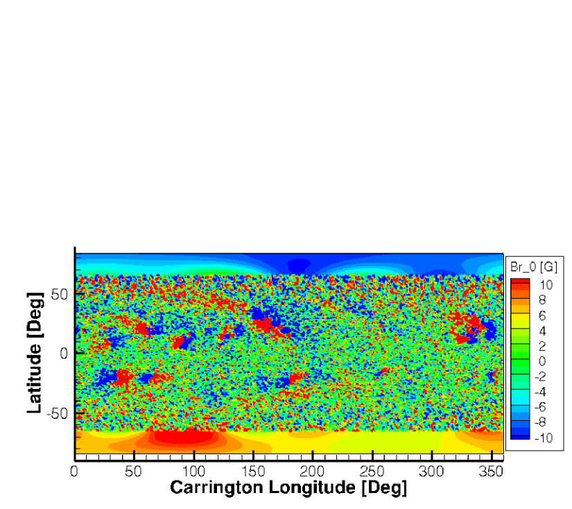
Figure 1: Carrington map of the radial magnetic field component at $1\;R_{\odot}$. This map is based on a synoptic magnetogram of CR2107 from SDO/HMI and processed to a PFSS solution using FDIPS. For the purpose of showing both the active regions and coronal holes, we have saturated the magnetic field in this plot at $\pm 10\;$G.

To simulate a background solar coronal solution, we need to specify the radial magnetic field component at the inner boundary, which is located in the upper chromosphere. We obtain this magnetic field in the following way: The synoptic map CR2107 of the SDO/Helioseismic and Magnetic Imager (HMI) is used. The polar field of this map is corrected with a two-dimensional and third-order polynomial fitting of the data above $60^{\circ}$ (Sun et al., 2013). We use FDIPS to generate an initial condition for the magnetic field and the boundary condition values for the radial magnetic field component (see Figure 1).

In all our results we will use parameter values as summarized in Table 1, unless stated otherwise. The boundary condition values are the same as in Sokolov et al. (2013). The value of $L_{\perp}\sqrt{B}$ is twice larger compared to the value used in Sokolov et al. (2013) due to a factor two difference in the definition of this parameter. The stochastic heating parameter $h_{s}$ and the collisionless heat conduction parameter $r_{H}$ are assigned with the same values as in Chandran et al. (2011).

3.1 Heat Partitioning

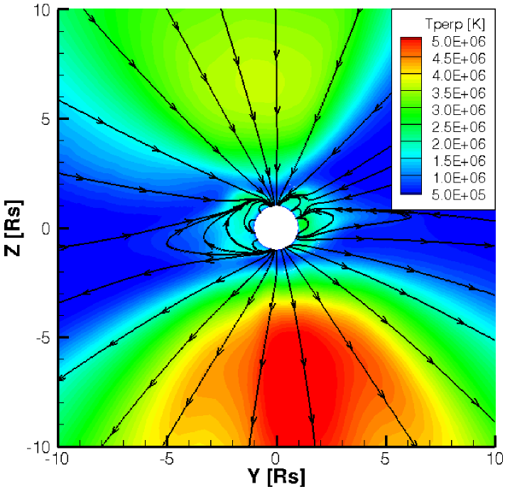
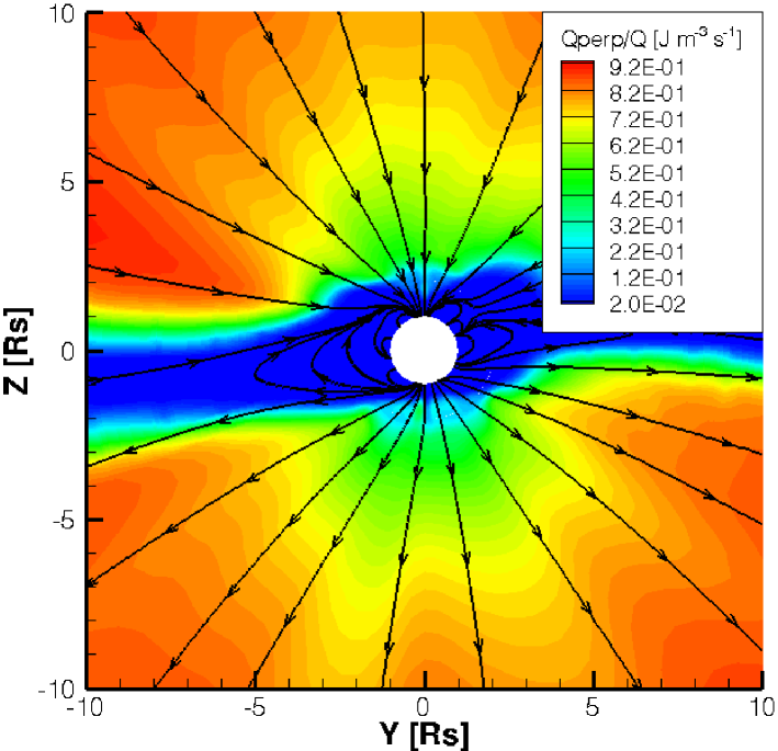
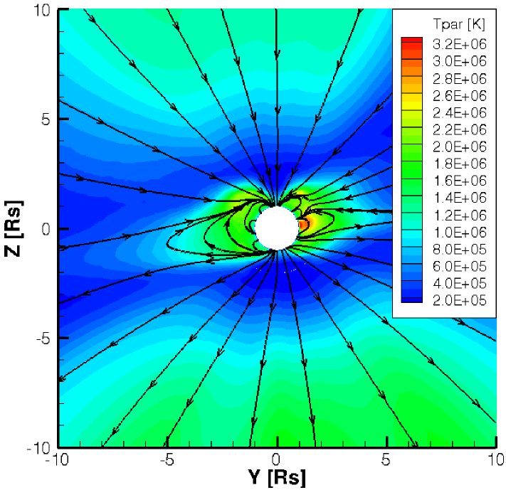
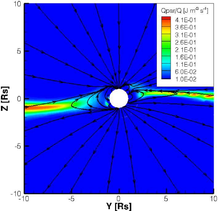
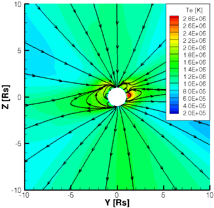
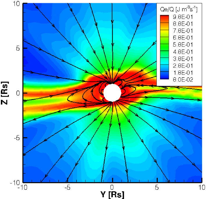
Figure 2: Meridional slice ($X=0$ plane from $-10\;R_{\odot}$ to $10\;R_{\odot}$) of the lower corona showing the three temperatures and heating fractions. Left panels (from top to bottom): perpendicular ion temperature, parallel ion temperature, and electron temperature in color contour, respectively. Streamlines represent field lines by ignoring the out-of-plane component. Right panels (from top to bottom): the ratio of the perpendicular ion, parallel ion, and electron coronal heating with the total turbulence dissipation.

We will first demonstrate the heat partitioning of the turbulence dissipation for our three-temperature model. In this simulation, we used the version of this model with the wave reflection term in Equations (11)–(17). The steady state solution is obtained with the spatially second-order shock-capturing scheme. In Figure 2, we show the three obtained temperatures $T_{i\perp}$, $T_{i\parallel}$, and $T_{e}$ from top to bottom in the panels on the left. These temperatures are shown in the meridional slice $X=0$ along with a few projected field lines to indicate the location of open and closed field lines. Very close to the Sun, the three temperatures are nearly the same. This is due to the high density near the Sun, resulting in a sufficiently high rate of Coulomb collisions that equilibrate the temperatures. The collision rate decreases with the density, so that further away from the Sun the collisions are too infrequent to equilibrate the temperatures. The significant heating of the perpendicular ion temperature in the polar coronal holes is due to the stochastic heating. The heat partitioning fractions of the coronal heating into ion perpendicular, ion parallel, and electron heating are shown in the panels on the right from top to bottom, respectively. The ion perpendicular heating, due to the stochastic heating process, dominates in the lower corona sufficiently far away from both the Sun and the heliospheric current sheet. The parallel ion heating is only significant very close to the heliospheric current sheet (HCS) due to the high plasma beta $\beta_{i}$, while the electron heating is important very close to the Sun and around the (HCS).

3.2 EUV Comparison

From the density and electron temperature distribution, calculated with our solar model, we can produce synthesized EUV that can be compared with the observed ones. Such a comparison serves as a check for the performance of the coronal heating model. The presented model accounts for the partial reflection of the outward propagating waves, which is accompanied by the generation of counter-propagating waves. These oppositely propagating waves are ultimately responsible for the turbulent cascade rate and hence, the coronal heating. The distinct feature in the present model is the enhanced reflection in the presence of strong magnetic fields, such as in close proximity of active regions, that can increase the dissipation and thereby intensify the observable EUV emission.

To better resolve the details in the synthesized LOS images, the latitudinal and longitudinal resolution is increased by using adaptive mesh refinement grid size of $6\times 6\times 6$. The first attempt to use the full model as described in Section 2 did not yet provide us the desired LOS image quality. The problem is due to the numerical inaccuracy in the Alfvén speed gradients in the reflection source term. To overcome this issue, we plan to solve the upper chromosphere and transition region semi-analytically in a forthcoming paper. In the present paper we changed for now to the turbulence model that is based on local dissipation in Equations (A4) and (A5) instead of the turbulence model with the wave reflection term in Equations (11)–(17). This model is less susceptible by these numerical errors.

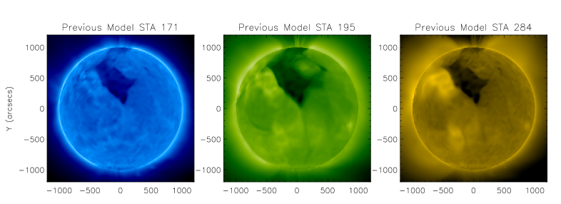
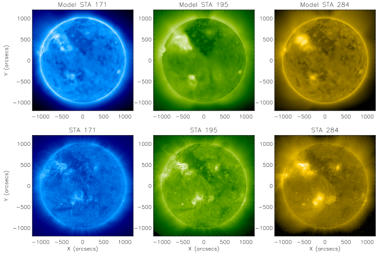
Figure 3: Comparison of synthesized EUV images of the model with observational STEREO A/EUVI images. The columns are from left to right for $171\;{\rm\AA}$, $195\;{\rm\AA}$, and $284\;{\rm\AA}$. Top panels: synthesized EUV images of the Sokolov et al. (2013) model. Midlle panels: synthesized EUV images of the improved model. Bottom panels: observational STEREO A/EUVI images. The observation time is 2011 March 7 20:00 UT.

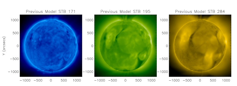
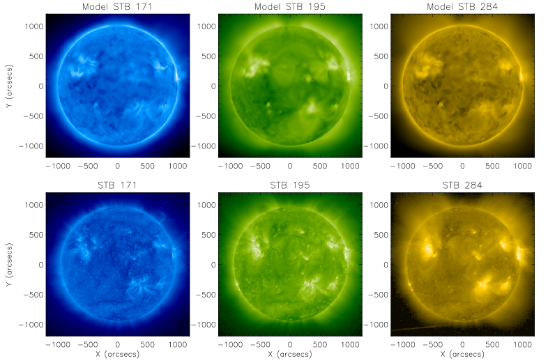
Figure 4: Comparison of synthesized EUV images of the model with observational STEREO B/EUVI images. The columns are from left to right for $171\;{\rm\AA}$, $195\;{\rm\AA}$, and $284\;{\rm\AA}$. Top panels: synthesized EUV images of the Sokolov et al. (2013) model. Midlle panels: synthesized EUV images of the improved model. Bottom panels: observational STEREO B/EUVI images. The observation time is 2011 March 7 20:00 UT.

In Figure 3, we computed the STEREO/EUVI emission images in the three coronal bandpasses for Fe emission lines at 171, 195, and $284\;$Å. These LOS images are produced by assuming that the plasma is optically thin for all the considered wavelengths. In the top row, the images are for the CR2107 steady solution of our previous model (Sokolov et al., 2013) using the spatially fifth-order MP5 limiter. In the middle row, we demonstrate the new model with the MP5 limiter. The new model better captures the active region emissivity as observed by the EUVI imager (Howard et al., 2008) on board STEREO A, as shown in the bottom panels. This enhanced emissivity is due to the increased reflection rate caused by the strong magnetic fields around active regions. We note that the steady state simulation was performed for a synoptic magnetogram, while the observation is for the time 2011 March 7 20:00 UT, and consequently, the model can not reproduce time dependent activity during the rotation. Also the polynomial extrapolation towards the pole in the CR2107 magnetogram might distort the high latitudinal region somewhat unfavorably. The observed polar coronal holes are somewhat wider than the coronal holes of the new model. In Figure 4, we similarly plot the results for STEREO B, which shows the other side of the Sun as the two STEREO spacecraft are separated by about 177 degrees. The emissivity of the active regions is, again, improved.

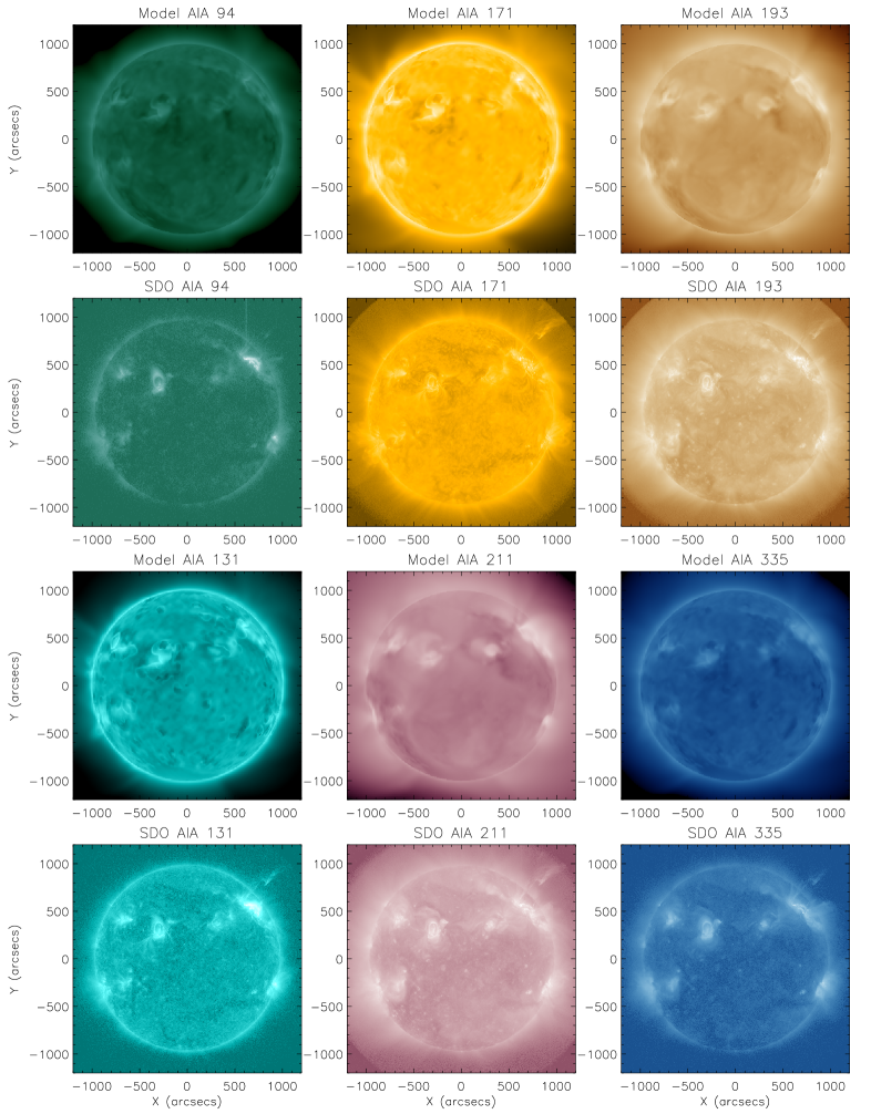
Figure 5: Comparison between synthesized AIA images of the model with the observed SDO/AIA images. Top panels (from left to right): AIA synthesized images for $94\;{\rm\AA}$, $171\;{\rm\AA}$, and $193\;{\rm\AA}$. Panels in second row: observational SDO/AIA images for those wavelengths. Panels in third row: AIA synthesized images for $131\;{\rm\AA}$, $211\;{\rm\AA}$, and $355\;{\rm\AA}$. Bottom panels: observational SDO/AIA images for those wavelengths. The observation time is 2011 March 7 20:00 UT.

In Figure 5, we show the comparison between the model synthesized SDO/AIA images with the images observed by AIA (Lemen et al., 2012) on board SDO. The model results are obtained with the MP5 limiter. The wavelengths indicated at the top of each panel correspond to various characteric temperatures. Again, the active regions are well captured.

4 CONCLUSIONS

We have presented our new AWSoM model. This solar model, which is part of the SWMF, is a three-dimensional Alfvén wave turbulence-driven model ranging from the upper chromosphere to the whole heliosphere. Compared to our previous models, AWSoM includes a generalization of the Alfvén wave turbulence to counter-propagating waves on both open and closed field lines. The outward propagating waves are now partially reflected by the Alfvén speed gradients and field-aligned vorticity. The balanced turbulence at the apex of the closed field lines is accounted for. We have also generalized our separate electron and ion temperature to anisotropic ion temperatures and isotropic electron temperatures. To distribrute the turbulence dissipation to the coronal heating of the three temperatures, we use the results of the linear wave theory and nonlinear stochastic heating as presented in Chandran et al. (2011). For the isotropic electron temperature, we have now also incorporated the collisionless heat conduction.

Our new model has no ad hoc coronal heating functions and has only a few adjustable parameters: three to prescribe the boundary conditions (density, temperature, and Poynting flux of the Alfvén waves), a transverse correlation length parameter for the turbulence and heat partitioning, a parameter related to the nonlinear stochastic heating of the ions, and two parameters for the collisionless heat conduction. Some of these parameters could potentially be described more self-consistently. For example, the transverse correlation length could be obtained from a time evolution equation (Breech et al., 2008) instead of the simple scaling with the magnetic field strength.

Since the evolution equations of our model do not assume open or closed field lines, those will develop self-consistently by using the data from photospheric magnetic field observations as boundary conditions for the magnetic field. The correctness of the coronal heating can be tested by comparing the simulated and observed multi-wavelength EUV images. We performed such a validation for CR2107. We demonstrated that our model can reproduce many features seen in the LOS images. The high latitudinal region is somewhat distorted. This might be an artifact due to the polynomial interpolation of the synoptic magnetogram above $60^{\circ}$ towards the pole. Future improvements in adapting magnetograms might address this issue. In our companion paper, X. Meng et al. (in preparation), we will showcase the model performance in the inner heliosphere by comparing the results for two Carrington rotations with in-situ observations at $1\;$AU.

Appendix A Model Simplification to Local Dissipation

We now consider the case that the turbulence is strongly imbalanced, i.e. $\min(w_{\pm})/\max(w_{\pm})\ll 1$. For simplicity, we also assume that $w_{+}$ is the dominant wave, and hence, $w_{-}$ is the minor wave ($w_{-}\ll w_{+}$). We can then simplify the wave equations (39) as

$$\frac{\partial w_{\pm}}{\partial t}+\nabla\cdot\left[({\bf u}\pm{\bf V}_{A})w_{\pm}\right]+\frac{w_{\pm}}{2}(\nabla\cdot{\bf u})=\mp{\cal R}_{\rm imb}\sqrt{w_{-}w_{+}}-\Gamma_{\pm}w_{\pm}.$$ (A1)

For the minor wave equation, only the right hand side of Equation (A1) has terms with the dominant wave. Hence, the reflection and dissipation term of the minor wave equation can, in leading order of the small quantity $w_{-}/w_{+}$, be assumed to be balanced. Using the dissipation rate $\Gamma_{-}=(2/L_{\perp})\sqrt{w_{+}/\rho}$, the minor wave energy density can then analytically be determined as $w_{-}=\frac{1}{4}\rho L_{\perp}^{2}{\cal R}_{\rm imb}^{2}$. Using this expression in the dissipation rate $\Gamma_{+}=(2/L_{\perp})\sqrt{w_{-}/\rho}$ of the dominant wave equation and further noting that, to leading order, the reflection term on the right hand side of Equation (A1) is much smaller than the dissipation term for the dominant wave, we arrive at the dominant wave equation

$$\frac{\partial w_{+}}{\partial t}+\nabla\cdot\left[({\bf u}+{\bf V}_{A})w_{+}\right]+\frac{w_{+}}{2}(\nabla\cdot{\bf u})=-{\cal R}_{\rm imb}w_{+},$$ (A2)

valid for strongly imbalanced turbulence. We note that the resulting equation only depends on the dominant wave energy density. A similar derivation can be performed when the $w_{-}$ is the dominant wave, and we combine both cases in a single formulation for strongly imbalanced turbulence:

$$\frac{\partial w_{\pm}}{\partial t}+\nabla\cdot\left[({\bf u}\pm{\bf V}_{A})w_{\pm}\right]+\frac{w_{\pm}}{2}(\nabla\cdot{\bf u})=-{\cal R}_{\rm imb}w_{\pm}.$$ (A3)

The exponentially small minor wave energy density is now assumed to be zero due to the absence of a reflection term in these evolution equations (although it could be recovered from the aforementioned analytical expression for the minor wave). Hence, by comparing Equations (A3) and (28), we can conclude that in strongly imbalanced turbulence, the dissipation rate is equal to the reflection rate, i.e. the wave dissipation is local. The dissipation does, in addition, no longer depend on the perpendicular correlation length. However, this derivation still dismisses the case that near the apex of closed field lines the wave energy densities can be of equal amplitude ($w_{+}\approx w_{-}$). For the balanced turbulence, the dissipation should still be estimated by the original expression (29). Combining both cases results in the final expression for the wave propagation and local dissipation

$$\frac{\partial w_{\pm}}{\partial t}+\nabla\cdot\left[({\bf u}\pm{\bf V}_{A})w_{\pm}\right]+\frac{w_{\pm}}{2}(\nabla\cdot{\bf u})=-\Gamma_{\pm}w_{\pm},$$ (A4)

in which the dissipation rate is

$$\Gamma_{\pm}=\max\left({\cal R}_{\rm imb},\frac{2}{L_{\perp}}\sqrt{\frac{w_{\mp}}{\rho}}\right).$$ (A5)

This approximation is valid for strongly imbalanced and balanced turbulence. The applicability to moderately imbalanced turbulence, for example in the transition region and chromosphere, is less certain.

Appendix B APPORTIONING ION AND ELECTRON HEATING

The partial reflection of the Alfvén waves due to Alfvén speed gradients and field-aligned vorticity generates counter-propagating waves. The nonlinear interaction between these oppositely directed waves results in an energy cascade from the large scale $L_{\perp}$ through the inertial range to the smaller perpendicular scales, i.e. larger perpendicular wavenumber $k_{\perp}$, where it can dissipate. The apportioning of the dissipated energy to the coronal heating functions $Q_{e}$, $Q_{i}$, and $Q_{i\parallel}$ depends on the microphysics that is involved. In this paper, we follow the partitioning strategy based on the dissipation of kinetic Alfvén waves (KAWs) using the theory described in Chandran et al. (2011). That formalism has the distinct advantage of providing approximated formulas that can readily be implemented in a numerical solar wind model that is based on the turbulent cascade of Alfvén waves. We have implemented those formulas in the present model, and below, we reproduce them for convenience.

In Chandran et al. (2011), the cascading of Alfvén waves transitions into cascading of KAWs. The KAWs can dissipate when $k_{\perp}r_{i}\sim 1$, where $r_{i}$ is the ion gyro radius. Among the dissipation mechanisms considered are the linear Landau damping and linear transit time damping of KAWs, which contribute to electron and parallel ion heating. The corresponding damping rates $\Gamma_{e}$ and $\Gamma_{i\parallel}$ are

$$\Gamma_{e}t_{c}=0.01\left(\frac{P_{e}}{P_{i}\beta_{i}}\right)^{1/2}\left[\frac{1+0.17\beta_{i}^{1.3}}{1+\left(2800\beta_{e}\right)^{-1.25}}\right],$$ (B1)

$$\Gamma_{i\parallel}t_{c}=0.08\left(\frac{P_{e}}{P_{i}}\right)^{1/4}\beta_{i}^{0.7}\exp\left(-\frac{1.3}{\beta_{i}}\right),$$ (B2)

where $\beta_{e}=2\mu_{0}P_{e}/B^{2}$ and $\beta_{i}=2\mu_{0}P_{i}/B^{2}$ are the electron and averaged ion plasma beta. Similar to Chandran et al. (2011), the Alfvén frequency $1/t_{c}=k_{\parallel}V_{A}$ for the parallel wavenumber $k_{\parallel}$ can be rewitten as $t_{c}=\rho\delta v_{i}^{2}/(\Gamma_{+}w_{+}+\Gamma_{-}w_{-})$ under the assumption of the critical-balance condition. The velocity perturbation $\delta v_{i}$ of the Alfvén waves and KAWs at $k_{\perp}r_{i}\sim 1$ is assumed to scale with $r_{i}/L_{\perp}$ via

$$\rho\delta v_{i}^{2}\approx w_{d}\sqrt{\frac{r_{i}}{L_{\perp}}},$$ (B3)

where $w_{d}=\max(w_{+},w_{-})$ is the dominant wave energy density. The minor wave energy density, $w_{m}=\min(w_{+},w_{-})$, is assumed to be exponentially small compared to $w_{d}$, which is, strictly speaking, not true in the balanced turbulence regime and hence, introduces some uncertainty in the heating partitioning. The above scaling is compatible with the $1\;$AU observations of Podesta et al. (2007). Furthermore, we assume similar to Chandran et al. (2011), nonlinear damping of KAWs via stochastic heating of ions, resulting in perpendicular ion heating. This energization is effective if $\delta v_{i}$ is large enough (Chen et al., 2001; Johnson & Cheng, 2001). This form of heating is the result of stochastic ion orbits perpendicular to ${\bf B}$ in an electrostatic potential. The damping rate for $\beta_{i\parallel}=2\mu_{0}P_{i\parallel}/B^{2}\lesssim 1$ is

$$\Gamma_{i\perp}=0.18\varepsilon_{i}\Omega_{i}\exp\left(-\frac{h_{S}}{\varepsilon_{i}}\right),$$ (B4)

where $\Omega_{i}=(e/m_{i})B$ is the ion gyro frequency, $v_{i\perp}=\sqrt{2P_{i\perp}/\rho}$ is the perpendicular ion thermal speed, $\varepsilon_{i}=\delta v_{i}/v_{i\perp}$, and $h_{S}$ is an input parameter for the stochastic heating. The heating functions are expressed in terms of the damping rates:

$$Q_{e}=\frac{1+\Gamma_{e}t_{c}}{1+(\Gamma_{e}+\Gamma_{i\parallel}+\Gamma_{i\perp})t_{c}}(\Gamma_{+}w_{+}+\Gamma_{-}w_{-}),$$ (B5)

$$Q_{i\parallel}=\frac{\Gamma_{i\parallel}t_{c}}{1+(\Gamma_{e}+\Gamma_{i\parallel}+\Gamma_{i\perp})t_{c}}(\Gamma_{+}w_{+}+\Gamma_{-}w_{-}),$$ (B6)

$$Q_{i}=\Gamma_{+}w_{+}+\Gamma_{-}w_{-}-Q_{e}.$$ (B7)

The $1+$ term in these expressions is for the remaining cascading power that succeeds to cascade to $k_{\perp}r_{i}\gg 1$, so that it can be assumed to be dissipated via interactions with electrons and hence, contributes to electron heating.

Appendix C COLLISIONLESS HEAT CONDUCTION

In this appendix, we will derive the final form of our implemented collisionless electron heat conduction. For convenience, we will limit the derivation to the inner heliosphere only, where the collisional heat conduction, Coulomb collisional heat exchange with the ions and the radiative cooling, can be neglected in the full electron energy equation (5). We additionally omit the time derivate as we focus in this paper on the steady state solar wind, and hence, Equation (5) can be simplified as

$$\nabla\cdot\left(\frac{p_{e}}{\gamma-1}{\bf u}\right)+p_{e}\nabla\cdot{\bf u}=-\nabla\cdot\left[\frac{3}{2}\alpha p_{e}{\bf u}\right]+Q_{e}.$$ (C1)

The first term on both the left hand side and the right hand side can be combined, resulting in

$$\nabla\cdot\left(\frac{p_{e}}{\gamma_{H}-1}{\bf u}\right)+p_{e}\nabla\cdot{\bf u}=Q_{e},$$ (C2)

where we have introduced a new polytropic index $\gamma_{H}$ for the electrons in the collisionless regime:

$$\gamma_{H}=\frac{\gamma+\frac{3}{2}(\gamma-1)\alpha}{1+\frac{3}{2}(\gamma-1)\alpha}.$$ (C3)

For our standard values $\alpha=1.05$ (taken from Cranmer et al. (2009)) and $\gamma=5/3$, we obtain $\gamma_{H}\approx 1.33$. By reintroducing the missing terms of Equation (5), we obtain our final evolution equation for the electron pressure:

$$\frac{\partial}{\partial t}\left(\frac{P_{e}}{\gamma_{e}-1}\right)+\nabla\cdot\left(\frac{P_{e}}{\gamma_{e}-1}{\bf u}\right)+P_{e}\nabla\cdot{\bf u}=-\nabla\cdot{\bf q}_{e}^{*}+\frac{N_{i}k_{B}}{\tau_{ei}}\left(T_{i}-T_{e}\right)-Q_{\rm rad}+Q_{e}.$$ (C4)

where

$$\gamma_{e}=\gamma f_{S}+\gamma_{H}(1-f_{S})$$ (C5)

interpolates the electron polytropic index $\gamma_{e}$ between the collisional regime where $\gamma_{e}=\gamma$ and the collisionless regime where $\gamma_{e}=\gamma_{H}$ and the interpolation function $f_{S}$ is taken to be the same as Equation (10). The $*$ in ${\bf q}_{e}^{*}$ indicates that we set ${\bf q}_{e,H}=0$ in the electron heat flux (9), i.e. ${\bf q}_{e}^{*}=f_{S}{\bf q}_{e,S}$, since it is now parameterized via a spatially varying $\gamma_{e}$.

The main difference between Equation (C4) and (5) is the use of $\gamma_{e}$ instead of $\gamma$ in the time derivative, and hence, the time evolution of both (ad hoc) formulations is different. As a final note, we mention that a spatially varying electron polytropic index does not negatively impact the shock evolution of coronal mass ejections (CMEs). Since the electron speed of sound is much larger than the CME speeds, only the ions will be heated by the CME shock. The ion fluid still uses the standard polytropic index $\gamma=5/3$.

Table 1: The model parameters.

Parameter	Value
$N_{\odot}$	$2\times 10^{17}\;{\rm m}^{-3}$
$T_{\odot}$	$50,000\;{\rm K}$
$(S_{A}/B)_{\odot}$	$1.1\times 10^{6}\;{\rm W}\,{\rm m}^{-2}\,{\rm T}^{-1}$
$L_{\perp}\sqrt{B}$	$1.5\times 10^{5}\;{\rm m}\,\sqrt{\rm T}$
$h_{S}$	0.17
$\alpha$	1.05
$r_{H}$	$5\;R_{\odot}$

References

- Alazraki & Couturier (1971) Alazraki, G., & Couturier, P. 1971, A&A, 13, 380
- Arge & Pizzo (2000) Arge, C.N. & Pizzo, V.J. 2000, J. Geophys. Res., 105, 10465
- Belcher & Davis (1971) Belcher, J.W., & Davis, L., Jr. 1971, J. Geophys. Res., 76, 3534
- Breech et al. (2008) Breech, B., Matthaeus, W.H., Minnie, J., et al. 2008, J. Geophys. Res., 113, A08105
- Chandran & Hollweg (2009) Chandran, B.D.G., & Hollweg, J.V. 2009, ApJ, 707, 1659
- Chandran et al. (2009) Chandran, B.D.G., Quataert, E., Howes, G.G., Xia, Q., & Pongkitiwanichakul, P. 2009, ApJ, 707, 1668
- Chandran et al. (2011) Chandran, B.D.G., Dennis, T.J., Quataert, E., & Bale, S.D. 2011, ApJ, 743, 197
- Chen et al. (2001) Chen, L., Lin, Z., & White, R. 2001, Phys. Plasmas, 8, 4713
- Cohen et al. (2007) Cohen, O., Sokolov, I.V., Roussev, I.I., et al. 2007, ApJ, 654, L163
- Coleman (1968) Coleman, P.J. 1968, ApJ, 153, 371
- Cranmer et al. (2009) Cranmer, S.R., Matthaeus, W.H., Breech, B.A., Kasper, J.C. 2009, ApJ, 702, 1604
- Cranmer (2010) Cranmer, S.R 2010, ApJ, 710, 676
- De Pontieu et al. (2007) De Pontieu, B., McIntosh, S.W., Carlsson, M., et al. 2007, science, 318, 1574
- Dmitruk et al. (2002) Dmitruk, P., Matthaeus, W.H., Milano, L.J., et al. 2002, ApJ, 575, 571
- Downs et al. (2010) Downs, C., Roussev, I.I., van der Holst, B., et al. 2010, ApJ, 712, 1219
- Evans et al. (2012) Evans, R.M., Opher, M., Oran, R., et al. 2012, ApJ, 756, 155
- Feng et al. (2010) Feng, X., Yang, L., Xiang, C., et al. 2010, ApJ, 723, 300
- Fichtner & Fahr (1991) Fichtner, H., & Fahr, H.J. 1991, A&A, 241, 187
- Heinemann & Olbert (1980) Heinemann, M., & Olbert, S. 1980, J. Geophys. Res., 85, 1311
- Isenberg (1984) Isenberg, P.A. 1984, J. Geophys. Res., 89, A86613
- Jin et al. (2012) Jin, M., Manchester IV, W.B., van der Holst, B., et al. 2012, ApJ, 745, 6
- Jin et al. (2013) Jin, M., Manchester IV, W.B., van der Holst, B., et al. 2013, ApJ, 773, 50
- Johnson & Cheng (2001) Johnson, J.R., & Cheng, C.Z. 2001, Geophys. Res. Lett., 28, 4421
- Hollweg (1978) Hollweg, J.V. 1978, Rev. Geophys. Space Phys., 16, 689
- Hollweg (1986) Hollweg, J.V. 1986, J. Geophys. Res., 91, 4111
- Hollweg & Kaghashvili (2012) Hollweg, J.V., & Kaghashvili, E.Kh. 2012, ApJ, 744, 114
- Hollweg et al. (2013) Hollweg, J.V., Kaghashvili, E.Kh., & Chandran, B.D.G. 2013, ApJ, 769, 142
- Howard et al. (2008) Howard, R.A., Moses, J.D., Voulidas, A., et al. 2008, Space Sci. Rev., 136, 67
- Hu et al. (2003) Hu, Y.Q., Habbal, S.R., Chen, Y., & Li, X. 2003, J. Geophys. Res., 108, 1377
- Kohl et al. (1998) Kohl, J.L., Noci, G., Antonucci, E., et al. 1998, ApJ, 501, L127
- Landi et al. (2013a) Landi, E., Young, P.R., Dere, K.P., Del Zanna, G., Mason, H.E. 2013a, ApJ, 763, 86
- Landi et al. (2013b) Landi, E., Oran, R., Gruesbeck, J.R., et al. 2013b, ApJ, submitted
- Leer & Axford (1972) Leer, E., & Axford, W.I. 1972, Sol. Phys., 23, 238
- Lemen et al. (2012) Lemen, J.R., Title, A.M., Akin, D.J., et al. 2012, Sol. Phys., 275, 17
- Leroy (1980) Leroy, B. 1980, A&A, 91, 136
- Li et al. (1998) Li, X., Habbal, S.R., Kohl, J., & Noci, G. 1998, ApJ, 501, L133
- Li et al. (2004) Li, B., Li, X., Hu, Y.-Q., & Habbal, S.R. 2004, J. Geophys. Res., 109, A07103
- Lionello et al. (2009) Lionello, R., Linker, J.A., & Mikić, Z. 2009, ApJ, 690, 902
- Manchester et al. (2012) Manchester IV, W.B., van der Holst, B., Tóth, G., & Gombosi, T.I. 2012, ApJ, 756, 81
- Marsch et al. (1982) Marsch, E., Schwenn, R., Rosenbauer, H., et al. 1982, J. Geophys. Res., 87, 52
- Mattheus et al. (1999) Matthaeus, W.H., Zank, G.P., Oughton, S., Mullan, D.J., & Dmitruk, P. 1999, ApJ, 523, L93
- McIntosh et al. (2011) McIntosh, S.W., de Pontieu, B., Carlsson, M., et al. 2011, nature, 475, 477
- Meng et al. (2012a) Meng, X., Tóth, G., Liemohn, M.W., Gombosi, T.I., Runov, A. 2012, J. Geophys. Res., 117, A08216
- Meng et al. (2012b) Meng, X., Tóth, G., Sokolov, I.V., & Gombosi, T.I. 2012, J. Comp. Phys., 231, 3610
- Odstrcil et al. (2005) Odstrcil, D., Pizzo, V.J., & Arge, C.N. 2005, J. Geophys. Res., 110, A02106
- Oran et al. (2013) Oran, R., van der Holst, B., Landi, E., et al. 2013, ApJ, 778, 176
- Podesta et al. (2007) Podesta, J.J., Roberts, D.A., Goldstein, M.L. 2007, ApJ, 664, 543
- Sokolov et al. (2013) Sokolov, I.V., van der Holst, B., Oran, R., et al. 2013, ApJ, 764, 23
- Sun et al. (2013) Sun, X., Liu, Y., Hoeksema, J.T., Hayashi, K., & Zhao, X. 2011, Sol. Phys., 270, 9
- Suresh & Huynh (1997) Suresh, S., & Huynh, H.T. 1997, J. Comp. Phys., 136, 83
- Suzuki & Inutsuka (2006) Suzuki, T.K., & Inutsuka, S.-i. 2006, J. Geophys. Res., 111, A06101
- Matsumoto & Suzuki (2012) Matsumoto, T., & Suzuki, T.K. 2012, ApJ, 749, 8
- Tóth et al. (2011) Tóth, G., van der Holst, B., & Huang, Z. 2011, ApJ, 732, 102
- Tóth et al. (2012) Tóth, G., van der Holst, B., Sokolov, I.V., et al. 2012, J. Comp. Phys., 231, 870
- Tu & Marsch (1995) Tu, C.-Y., & Marsch, E. 1995, Space Sci. Rev., 73, 1
- Usmanov et al. (2000) Usmanov, A.V., Goldstein, M.L., Besser, B.P., & Fritzer, J.M. 2000, J. Geophys. Res., 105, 12675
- van der Holst et al. (2010) van der Holst, B., Manchester IV, W.B., Frazin, R.A., et al. 2010, ApJ, 725, 1373
- van der Holst et al. (2011) van der Holst, B., Tóth, G., Sokolov, I.V., et al. 2011, ApJS, 194, 23
- van der holst et al. (2013) van der Holst, B., Tóth, G., Sokolov, I.V., et al. 2013, High Energy Density Physics, 9, 8
- Vásquez et al. (2003) Vásquez, A.M., van Ballegooijen, A.A., & Raymond, J.C. 2003, ApJ, 598, 1361
- Velli et al. (1989) Velli, M., Grappin, R., & Mangeney, A. 1989 Phys. Rev. Lett., 63, 1807
- Velli (1993) Velli, M. 1993, A&A, 270, 304
- Verdini & Velli (2007) Verdini, A., & Velli, M. 2007, ApJ, 662, 669