Coexisting itinerant and localized electrons
Abstract
The surprising discovery of high- superconductivity in iron-based compounds has prompted an intensive investigation on the role of interaction and magnetism in the these materials. Based on the general features of multi-bands and intermediate coupling strengths, a phenomenological theory of coexisting itinerant and localized electrons has been proposed to describe the low-energy physics in iron-based superconductors. It provides a unified framework to understand magnetic, superconducting, and normal phases, subject to further microscopic justification and experimental verification.
I Introduction
In the past five years, the study of iron-based superconductors have attract much attention in the condensed matter community and beyond. These new superconductors contain the FeAs/FeSe active layers, and the first principle calculationsHaule et al. (2008); Ma and Lu (2008); Kuroki et al. (2008); Singh (2008); Subedi et al. (2008) have shown that the electrons from the iron orbitals dominate the density of states at the Fermi energy.
One key issue under early debate is about whether the iron electrons should be treated as itinerant electrons or local moments. Underlying this dispute are the two different schools of thought about the mechanism for superconductivity: the Bardeen-Cooper-Schieffer (BCS) theory in a weakly interacting metalBardeen et al. (1957a, b) versus the resonating valence bound (RVB) type of theory for a strongly correlated system like the cuprate.Anderson (1987); Anderson et al. (2004)
The BCS theory is based on a weakly correlated Fermi liquid state of itinerant electrons. At low temperatures, a Fermi liquid state will become unstable against any weak attractive interaction, which drives the electrons near Fermi surface to form Cooper pairs and condense, giving rise to superconductivity. The effective attraction can be either mediated by phononsBardeen and Pines (1955), plasomonsKohn and Luttinger (1965), magnonsBerk and Schrieffer (1966); Doniach and Engelsberg (1966) etc., or originated from the bare electron interaction via the fluctuation-exchangeBickers and Scalapino (1989) (FLEX) or the renormalization groupShankar (1994) (RG) approaches. To make the attraction dominant at low-energy, the Coulomb repulsion must be effectively screened, which in turn requires the electrons be itinerant, such that the BCS theory usually works for a system of metallic normal state.
On the other hand, in a strongly correlated system like the cuprate,Anderson (1987); Anderson et al. (2004) the electrons can be localized, due to the strong Coulomb interaction, to form a Mott insulator at half-filling. Here its charge degree of freedom is gapped, while the remaining spin degree of freedom forms a lattice of fluctuating local moments. Superconductivity arises upon charge doping into the Mott insulator. The failure of a conventional BCS theory lies in that the Coulomb repulsion becomes a dominant effect in shaping the electronic state instead of simply getting screened in the BCS theory. In such a single-band strongly correlated system, electron fractionalization is a natural consequence in which doped charges and localized spins behave distinctly as separated degrees of freedom. The underlying mechanism for superconductivity is generally known as an RVB theory because the singlet pairing of the local moments becomes partially charged upon doping, resembling the Cooper pairing,Anderson (1987) to give rise high- superconductivity.
While the BCS theory and the RVB theory lie in the opposite extremes of the electron correlations, most of studies seem to agree on that the iron-based compound is an intermediate correlated electron system.Qazilbash et al. (2009); Johnston (2010) In particular, the multi-band iron electrons are involved in the low-energy sector in contrast to the single-band electrons in the cuprate. As to be discussed in this Chapter, a new possibilityKou et al. (2009) may arise in the low energy regime of the iron-based superconductor, in which the multi-band electrons effectively behave as if some of them still remain itinerant near the Fermi energy and some of them become more localized like in a Mott insulator. Such a “fractionalization” into two more conventional subsystems of itinerant and localized electrons in a multi-band case is in sharp and interesting contrast with a novel fractionalization of electrons in a single band doped Mott insulator. Here, without doping into the Mott insulator, the itinerant electrons remain effectively separated from the local moments as independent degrees of freedom, and two subsystems mutually interact with an intermedate coupling strength, which can be tractable perturbatively. In the following, relevant experimental facts and theoretical approaches will be briefly overviewed.
I.1 Basic Experimental Evidence
The experimental evidence for the simultaneous presence of both itinerant electrons and local moments has been manifested in almost all families of iron-based superconductors.
I.1.1 Itinerant Electrons
An early direct experimental fact that supports the existence of itinerant electrons in the iron-based compounds is the semi-metal behavior even in the magnetically ordered phase. For most families of the materials,Kamihara et al. (2008); Ren et al. (2008a, b); Chen et al. (2008a); Kito et al. (2008); Tapp et al. (2008); Sefat et al. (2008); Rotter et al. (2008); Wang et al. (2008, 2008); Sales et al. (2009); Chen et al. (2009); Chu et al. (2009) it has been observed that the resistivity decreases as the temperature is lowered, as shown in Fig. 1 (taking the 122-familyFang et al. (2009) as an example), a typical behavior of a metallic system, contrary to the insulating and localization behavior generically observed in the undoped and lightly doped cuprates in the magnetically ordered phase.
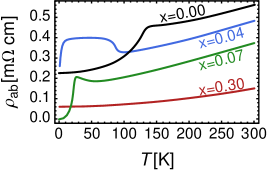
A finite residual resistivity of the parent compound, of the order mcm at low limit, is shown in Fig. 1 (the same order of resistivity is also observed in the 111-familyTapp et al. (2008) and the 11-familySales et al. (2009)). According to the analysis in Refs. Si and Abrahams, 2008; Johnston, 2010, for a two-dimensional electron system, the in-plane resistivity is related to the electron mean-free-path by , where is the Fermi momentum, and is the distance between the conducting layers (which is Åfor the 122-family). According to this estimate, the in-plane electron mean-free-path can be as long as ,Johnston (2010) indicating a nice coherence of the quasiparticles around the Fermi surface, which can be identified as well-defined itinerant electrons.
The band structure obtained by the first principle calculationsSingh and Du (2008); Cao et al. (2008); Ma and Lu (2008); Kuroki et al. (2008) shows that all the five iron orbitals are close to each other in energy, and the density of states near the Fermi energy are mainly contributed by the Fe orbitals. The electron and hole Fermi pockets predicted in the band structure calculation are clearly confirmed by angular resolved photoemmision spectroscopy (ARPES) experiments.Liu et al. (2008) Although a renormalization factor of is usually requiredLu et al. (2009); Cui et al. (2012) to account for the experimental data, which may be due to correlation effect, the fact that there are itinerant electron bands going across the Fermi level is well established. Moreover, the observed broadening of the energy spectrum gets progressively reduced approaching the Fermi level,Liu et al. (2008); Lu et al. (2009); Cui et al. (2012); Vilmercati et al. (2009); Xia et al. (2009); Borisenko et al. (2010); He et al. (2010) which implies asymptotically better quasiparticle coherence. This asymptotic coherence is a typical Landau Fermi-liquid behavior. Similar behavior is also shownAichhorn et al. (2009) in the dynamic mean-field theory (DMFT) calculations.
The quantum oscillation observed in the 1111-familyColdea et al. (2008) and 122-familySebastian et al. (2008); Coldea et al. (2009); Analytis et al. (2009a, b) lends further support to the itinerant electron coherency around the Fermi surface. The measurementColdea et al. (2009) also shows that the mean-free-path of the itinerant electrons can reach the order of 1000Å, which is much larger than the lattice constant (Å). Even in the spin-density-wave (SDW) ordered magnetic parent compounds, because the SDW state is not fully gapped,Ran et al. (2009) quantum oscillation experiment can still detect the residual Fermi surface and confirm the quasi-particle coherenceAnalytis et al. (2009b) in the magnetically ordered state.
The SDW gap opened up from the reconstruction of the itinerant electrons near the Fermi pockets has been also observed in both the scanning tunneling microscopy (STM) and optical conductivity measurements. An SDW gap of meV is found in the STM experimentZhou et al. (2012) with the gap bottom deviating from the Fermi level due to imperfect nesting. The optical conductivity experimentsHu et al. (2008); Moon and Choi (2010); Moon et al. (2010); Wang et al. (2012) observed a low-energy spectral weight transfer in the SDW transition. However both the STMZhou et al. (2012) and the optical conductivityMoon et al. (2010) measurements have also indicated an energy gap feature (eV) substantially larger than the SDW gap, which is present over a much higher temperature and wider doping regime covering both SDW and superconducting (SC) phases. This latter energy scale may be considered to be a generalized Mott gap which protects some effective local moments, implying the coexistence of both itinerant and localized electrons in the system. In the following, the experimental evidence for the presence of local moments will be briefly discussed.
I.1.2 Local Moments
The elastic neutron scattering (ENS) study of the magnetically ordered parent compounds has shown that the ordered moment per Fe atom, , varies significantly among the materials: in the 1111-familyde La Cruz et al. (2008); Chen et al. (2008b); Kimber et al. (2008); Qiu et al. (2008); Zhao et al. (2008a); Xiao et al. (2009a, 2010); Tian et al. (2010), in the 122-familyGoldman et al. (2008); Zhao et al. (2008b); Kaneko et al. (2008); Huang et al. (2008); Matan et al. (2009); Wilson et al. (2009); Xiao et al. (2009b), and in the 11-familyLi et al. (2009a); Bao et al. (2009); Martinelli et al. (2010); Liu et al. (2010). One may consider the relatively small magnetic moment (compared to that of the Fe2+ ionCao et al. (2008)) observed in the iron-based compounds as an evidence for the itinerant magnetism. However the opposite opinion argues that not all the -orbital electrons participate in the formation of the local moment, as some of them may remain itinerant around the Fermi surface such that a local moment should not be simply deduced from an Fe2+ ion model. Further, the ordered moment is subject to the magnetic fluctuation,Si and Abrahams (2008); Rodriguez and Rezayi (2009); Hansmann et al. (2010) which is averaged over the observation timescale, and is always smaller than an instant moment.
An instant (high energy scale) moment at the iron atom can be directly measured by the x-ray emission spectroscopyGretarsson et al. (2011); Vilmercati et al. (2012) (XES), in which the measurement timescale is of s, much faster than the timescale s of the Mössbauer spectroscopy, the nuclear magnetic resonance (NMR) and the muon spin resonance (SR), and is also faster than the ENS timescale by orders of magnitude. So the XES measurement probes the instant magnetic moment at a time scale much shorter than that of magnetic correlations established among the local moments as probed in the ENS experiment. The XES resultGretarsson et al. (2011) shows that even at room-temperature, a local magnetic moment can still be detected, which is about (corresponding to the spin ) for the 1111-, 122- and 111-families, and for the 11-family. It is further discovered that the local moment exists in all phases including the magnetically disordered phases as well as the paramagnetic (PM) and SC phases.
Here the size of the local moment is insensitive to the temperature variation, which excludes the possibility that these moments are originated from itinerant magnetism. A careful experiment studyVilmercati et al. (2012) discovers that the local moment varies in different phases. The measured in the PM/SC phases of the optimal doped Sr(Fe1−xCox)2As2() is reduced by half as compared to of the parent compound SrFe2As2 in the SDW phase at 17K, as if the local moment spin is reduced from in the SDW phase to in the PM/SC phase, indicating the possibility of spin fractionalization of the local moment outside the SDW phase.
Other indirect evidences for the existence of local moments include that the nuclear hyperfine splitting in the Mössbauer spectrumBonville et al. (2010) persists up to (where stands for the SDW transition temperature), and that a well-defined spin-wave spectrum observed in the inelastic neutron scattering (INS) experimentsZhao et al. (2009); Xu et al. (2011) extends up to the energy scale of 200meV (). The pure itinerant electron picture can hardly account for the high-energy/high-temperature magnetism, when the SDW order ceases to exist.
Mover, the NMR Knight shiftNing et al. (2009); Imai et al. (2009); Ning et al. (2010); Michioka et al. (2010); Ma et al. (2011) and uniform suspectibilityYan et al. (2008); Wu et al. (2008); Wang et al. (2009a); Klingeler et al. (2010) experiments have both observed the linear temperature dependence of the magnetic susceptibility all the way to above 500-800K. Such behavior can be explainedZhang et al. (2009); Kou et al. (2009) by the antiferromagetic (AFM) short-range correlation between local moments. Here the experiments once again indicate the persistence of the local moments with AFM correlations up to much higher temperatures than .
I.2 Theories for Iron-Based Superconductors
In general, there are three schools of theories: itinerant theoryMazin et al. (2008); Yildirim (2008); Chubukov et al. (2008); Sknepnek et al. (2009); Maier et al. (2009); Wang et al. (2009b); Zhai et al. (2009); Ummarino et al. (2009), localized theorySi and Abrahams (2008); Seo et al. (2008); Craco et al. (2008); Haule and Kotliar (2009); Laad et al. (2009); Abrahams and Si (2011); Hu and Ding (2012); Yu and Si (2012); Flint and Coleman (2012) and the hybrid theory of coexistent itinerant and localized electronsWeng (2009); Kou et al. (2009); Yin et al. (2010); Lv et al. (2010); Gor’kov and Teitel’baum (2013), see Tab. 1.
| Itinerant electron | Local moment | Hybrid | |
|---|---|---|---|
| Degrees of freedom | Itinerant electrons | Local moments | Coexistence of both |
| Electron correlation | Weak | Strong | Intermediate |
| Starting point | Fermi liquid | Mott insulator | Orbital-selective Mott |
| SC mechanism | BCS pairing | Spin RVB pairing | BCS pairing |
| Pairing glue | Electron collective fluctuation | Superexchange | Local moment fluctuation |
The itinerant theory is built on the picture of pure itinerant electrons, which views the iron-based superconductor as a simple BCS superconductor with the electron pairing mediated by spin-fluctuations generated by the interaction among itinerant electrons. The local theory takes a strong correlation point of view and considers the iron-based superconductor as a multi-band version of doped Mott insulators similar to the cuprates. The coexistence theory emphasizes that itinerant electrons and local moments should both exist in the iron-based materia, as independent degrees of freedom at least in the low-energy sector. A careful differentiation of these theories and their underlying physics is important in search for the correct microscopic mechanism of superconductivity, as to be detailed below.
I.2.1 Itinerant Electron Theory
Starting from the -orbital itinerant electron bands, and combining with the intra-atomic interaction, one can establish the multi-band Hubbard modelRaghu et al. (2008); Chubukov et al. (2008); Lee and Wen (2008)
| (1) |
where is the electron operator of the orbital on the site, which contains two spin components and . Here is the charge density operator, is the spin operator, and is the pairing operator. describes the hopping of electron, in which the hopping coefficient can be obtained from the band structure calculationKuroki et al. (2008), or determined by fitting the ARPES observed band structure. describes the electron interaction inside the iron atom, including the the intra-orbital repulsion , the inter-orbital repulsion , and the Hunt’s rule exchange interaction and the pair-hopping interaction .
Based on the multi-band Hubbard model, an itinerant theory starts from the electron band structure in , and treats the interaction term perturbatively. The simplest treatmentSknepnek et al. (2009); Maier et al. (2009) includes the calculation of the spin susceptibility function in the RPA framework, where stands for the interaction vertex given by , while the bare spin susceptibility can be calculated from the band structure by where denotes the Fermi function. The obtained from the RPA calculation reflects the collective spin fluctuation of itinerant electrons under weak interaction. According to the Berk-Schrieffer theory,Berk and Schrieffer (1966) the spin fluctuation can mediate pairing interaction between electrons, as , where is the Cooper pair operator. Plugging this interaction into the Eliashberg gap equation,Ummarino et al. (2009) one can obtain the form factor of , and estimate the superconductivity transition temperature. Following this line of thought, Mazin and collaboratorsMazin et al. (2008) first predicted the -wave pairing symmetry in the iron-based superconductor, which is consistent with many experiments. Thus the spin-fluctuation BCS theoryScalapino et al. (1986); Pines (1997a, b) previously developed for the cuprate superconductors thrives again in the study of iron-based superconductors. The simple RPA calculation can be improved to a self-consistent FLEX calculation.Yu et al. (2009); Yao et al. (2009) Or one can use the RG approachesChubukov et al. (2008); Chubukov (2009); Wang et al. (2009b); Zhai et al. (2009) to track the flow of the interaction vertex towards the low energy scale, so as to analyze the competition between different orders.
Besides the SC phase, the SDW phase may also be understood within the itinerant electron theory. Due to an approximate nesting of the Fermi pockets, the spin fluctuation becomes the strongest near the nesting momentum, which is consistent with the collinear antiferromagnetic (CAFM) order in most parent compounds. In an itinerant electron theory, SDW and SC can compete and coexist.Vorontsov et al. (2009, 2010); Fernandes and Schmalian (2010) However more concrete calculation by the FLEX methodArita and Ikeda (2009) shows that starting from a purely itinerant picture, it is hard to obtain robust enough CAFM order in a reasonable parameter regime, which implies the importance of local moments in stabilizing the SDW phase.
I.2.2 Local Moment Theory
In view of the bad metal behavior, many considerSi and Abrahams (2008); Craco et al. (2008); Haule and Kotliar (2009); Laad et al. (2009); Abrahams and Si (2011); Flint and Coleman (2012) the parent compounds of iron-based superconductors to be proximate to Mott insulators. In other words, the materials are in strongly correlated regime, in contrast to a weakly correlated itinerant electron description outlined above. Based on this idea, a mutiband -- modelSi et al. (2009) has been proposed:
| (2) |
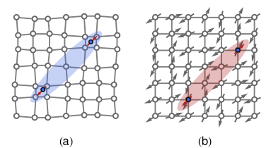
where in the electron operator , the spin and orbital degrees of freedom are implicitly implied, and stands for the local moment at the site made up by the localized electrons. The superexchange interaction between the local moments is described by . The CAMF order in the SDW phase can be reasonably explained by considering the nearest neighboring coupling and the next nearest neighboring coupling .Si and Abrahams (2008) describes the hopping of doped electrons on the lattice, and the projection operator restricts the on-site electron configuration in the physical Hilbert space to distinguish the local moment and doped charge (which can be regarded as a multi-band generalization of the no-double-occupancy condition in the single-band Hubbard model).
Because of the projection operator , one can no longer simply treat in Eq. (2) as describing itinerant electrons like in of Eq. (1). In other words, enforces strong correlations in the -- model. One way to tackle the -- model is to introduce the so-called U(1) slave boson approach.Flint and Coleman (2012) In a fashion similar to the one-band - model, based on the picture of spin-charge separation, here the electron operator may be fractionalized into a product of the fermionic spinon and the bosonic chargon as , under the equal-density constraint of the spinon and the chargon . In the SC phase, the chargons are condensed , so that at the mean-field level, the spinon dynamics follows , where . For the zero-momentum condensate of chargons, we roughly have , meaning that the spinon shares the same band structure as the itinerant electrons in Eq. (1). actually describes a spinon Fermi-liquid with magnetic interaction . In the momentum space, the magnetic interaction effectively becomes a pairing interaction among the spinons , where , and representes the spin-singlet pairing operator of spinons. The CAFM order of the parent compounds implies that the next nearest neighboring antiferromagnetic exchange interaction is dominant. While in the momentum space, interaction corresponds to , which is attractive in the long range, and repulsive in the short range (where is the nesting momentum between the hole and the electron pockets in the iron-based compounds). This interaction combined with the band structure would naturally give rise to the -wave pairing symmetry, i.e. the pairing order parameter remains the same sign within the same pockets so as to gain energy in the channel, while the pairing sign becomes opposite between the pockets connected by as favored by the channel. Under the chargon condensation, the pairing of the electron directly follows from the spinon pairing , such that the experimentally observed -wave pairing of the electrons may be similarly understood in the slave-boson theory.
The above analysis indicates a close relation between the magnetic fluctuations of the local moments and the pairing symmetry in iron-based superconductors. The short-ranged CAFM fluctuation, with a momentum that connects the electron and the hole pockets, would always lead to the -wave pairing symmetry. Thus for both the itinerant electron theory and the local moment theory, the same conclusion on the pairing symmetry can be reached.Mazin and Schmalian (2009); Hu and Ding (2012) However, just like in the high- cuprate, the pairing symmetry itself is not enough to resolve the mechanism for superconductivity.
I.2.3 Hybrid Theory
The itinerant theory holds the point of view of weak electron correlations, while the local moment theory stresses strong electron correlations where all the electrons are in or proximate to the (doped) Mott insulator regime. Two pictures are in opposite limits: i.e., itinerant vs. localized electrons. In the latter case, the metallicity of doped electrons no longer simply behaves like that of itinerant electrons obtained by a band structure calculation because under the projection operator in Eq. (2), now the electrons have to always remember that part of them are localized moments. This has been the very key issue in the study of doped Mott insulator, and generally a spin-charge separation or fractionalization of the electron seems to result as the natural consequence of such strong correlations as mentioned above.
However, in contrast to the cuprate superconductors, the iron-based superconductors are the multi-band materials with intermediate coupling strengths, which opens door for a new possibility. Given the experimental facts that the itinerant electrons and local moments are both well established in different channels of measurements as seen above, it is sensible to make a phenomenological hypothesis that may be both degrees of freedom, i.e., itinerant electrons and localized moments, can spontaneously emerge from the 3 electron bands after some intermediate strength interactions in Eq. (1) has been taken into account. Namely, in an RG sense, the following phenomenological modelWeng (2009); Kou et al. (2009); Yin et al. (2010) may become relevant to the low-energy physics of the iron-based superconductors
| (3) |
where captures the itinerant electron band structure which determines the Fermi pockets observed in the ARPES, describes the superexchange couplings between the local moments denoted by , and accounts for the simplest residual interaction between the itinerant electrons and the local moments: a renormalized Hund’s rule ferromagnetic coupling .
If the effective Hund’s rule coupling is sufficiently weak, the Hamiltonian (3) simply reduces to two independent states: a Fermi liquid of itinerant electrons and a short-range CAFM state of the local moments, consistent with the observed normal state of the iron-based superconductors. The ferromagnetic coupling between the itinerant electrons and the local moments tends to align their spins/magnetic moments in the same direction. If the Fermi surfaces are reasonably well nested, a strong SDW instability will occur to the itinerant electrons by even weakly coupling to the short-ranged CAFM correlation of the local moments. Furthermore, such an SDW order is under a strong competition form the Cooper pairing instability, because by the same coupling term the itinerant electrons also tend to pair by exchanging the collective magnon mode of the local moments, as illustrated in Fig. 2, in analogy to the conventional phonon-glue BCS superconductor. Because the magnon energy scale (meV) is much higher than that of conventional phonons, the transition temperature of the magnon-glue BCS superconductivity may exceed the McMillan limit to give rise to a higher .
It is important to distinguish Eq. (3) from Eq. (2) as they represent drastically different low-energy physics. In the effective theory of Eq. (3), the itinerant electron creation operator and the local moment operator are independent degrees of freedom, whereas in Eq. (2) and are the operators for the same electrons. In particular, the strong correlation nature of Eq. (2) is enforced by the Gutzwiller projection operator . In other words, a simple-minded relaxation of it in Eq. (2) could result in a totally different weak-correlation physics: i.e., an itinerant electron system interacting with perturbative coupling strength, , where there is no trace of local moments anymore!
The hybrid theory shares with the itinerant theory that both the SDW and SC orders are formed by the same itinerant electrons. But in the former, the driving force for both SDW instability and the pairing glue comes from coupling to the local moments, whose correlations can persist over a wide temperature and doping regime. In the itinerant theory, however, the SDW instability is driven by the Fermi surface nesting and the pairing glue is attributed to spin fluctuations of the itinerant electrons themselves. Beyond a narrow transition region of the SDW order, such spin fluctuations usually damp quickly, and the Cooper pairing of the itinerant electrons could further suppress the spin fluctuations self-consistently.
Although the debate on the roles of itinerant electrons and local moments has not been settled completely, it seems that the the consensus is converging to the picture of coexistence in order to account for a vast range of experiements. The introduction of two independent degrees of freedom in the hybrid model is not to complicate the problem, but to separate the different roles played by the iron electrons, which in turn simplifies the phenomenological description of the iron-based superconductors. Here the itinerant electron and the local moment may be regarded as the emergent degrees of freedom in the multi-band Hubbard model Eq. (1) at low energy, resulting from the so-called orbital-selective Mott transition to be discussed below.
I.2.4 Orbital Selective Mott Transition
The descriptions of itinerant electrons and local moments are distinguished by the Mott transition. The study of Mott transition has a history of more than half a century.Gutzwiller (1963); Hubbard (1963) The discovery of the cuprate superconductors has motivated an extensive study of the single-band Hubbard model. It has been demonstrated in the DMFT and quantum Monte-Carlo (QMC) calculationsGeorges et al. (1996) that there exists an intermediate correlated region where the Mott transition takes place. However, the presence of an SDW/AFM ordering in the itinerant/local moment regime may mask such a transition at low temperatures for a single-band Hubbard model, say, on square lattice.
On the other hand, because the iron-based superconductor is not only intermediate-correlated but also possesses multiple bands in the electronic structure, a new possibility arises beyond the two simple classifications of itinerant and localized electrons. Here the multi-band structure combined with the intermediate correlation may lead to a new kind of Mott transition: the orbital-selective Mott (OSMott) transition.de’Medici et al. (2009); Hackl and Vojta (2009); Vojta (2010); de’Medici (2011); Yu and Si (2011); Zhang et al. (2012); Quan et al. (2012); Yu and Si (2012) With the OSMott transition, different electron bands will exhibit distinct characteristics of itineracy and Mott localization, which supports the previously outlined hybrid theory of coexisting itinerant electrons and local moments.
The studiesHaule and Kotliar (2009); Johannes and Mazin (2009); de’Medici (2011); Quan et al. (2012) have demonstrated that the Hund’s rule coupling between the on-site -orbital electrons plays an important role in driving the OSMott transition together with the Coulomb repulsion . The Hund’s rule coupling tends to align the electron spins from different orbitals into the same direction, which enhances the electron correlation and the formation of local moments.Johannes and Mazin (2009); Wang et al. (2010) Fig. 3 displays the phase diagram of the multi-band Hubbard model obtained by the DMFTde’Medici et al. (2009) calculation. The reader is referred to the next Chapter of this book for the detailed theoretical discussion of OSMott transitions.

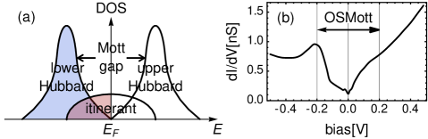
The OSMott state is characterized in the electron density of states by the coexisting itinerant band and the Hubbard bands (with the OSMott gap), as illustrated in Fig. 4(a). The itinerant electrons contribute to a finite density of states at the Fermi energy, governed by the weakly correlated physics, while the local moments have no direct contribution at the Fermi energy, as if there is a generalized Mott gap. On the other hand, the local moment degree of freedom will dominate the low-lying spin fluctuations in the magnetic channel. The coexistence of weakly and strongly correlated components is supported by the opticalMoon et al. (2010); Wang et al. (2012) and STM Zhou et al. (2012) experiments in the iron-based compound. In the BaFe2As2 compound, the optical measurementWang et al. (2012) has revealed a charge transfer gap of the energy scale 0.6eV opening up at low temperature. Similar large gap feature of eV has been directly observed in the STM differential conductance spectrum of NaFe1-xCoxAs compounds,Zhou et al. (2012) as shown in Fig. 4(b), where a V-shaped like feature associated with this large Mott-like gap is “pinned” at the Fermi energy, with a finite zero-bias density of states of the itinerant electrons where the smaller SDW and SC gaps are found at low temperatures at different ’s. With the increase of , the electrons are doped into the FeAs layer which seem all entering the itinerant bands, leading to their rigid band shift. On the other hand, the high-energy V-shaped curves remains unchanged and pinned at the Fermi level,Zhou et al. (2012) indicating that no significant doped charges go to the Mott localized bands, lending support to Fig. 4(a) and the hybrid model of Eq. (3).
II Two-Fluid Description for Iron-Based Superconductors
In the Introduction, we have given both experimental evidence and theoretical consideration justifying a phenomenological description of the iron-based superconductor, namely, the coexisting itinerant and localized electrons or the so-called hybrid theory. In this section, we shall present a detailed and systematic model study along this line of thinking, which provides a unified understanding for the basic physics of magnetism and superconductivity in the iron-based materials.
II.1 Two-Fluid Description Based on the Hybrid Model
In the hybrid theory, the minimal model of Eq. (3) is a mixture of the weakly correlated Fermi liquid physics of itinerant electrons and the strongly correlated Mott physics of local moments. Without doping into the local moment degree of freedom, the charge carriers remain in a Fermi liquid state, which is much simplified as compared to the doped - type model in Eq. (2).
The study of Eq. (3) in various parameter regimesKou et al. (2009); You et al. (2011a) has demonstrated that the hybrid theory is capable of explaining the SDW and SC ordered phases as well as the normal state properties in the iron-based superconductors. However, in order to accommodate the experiments of the iron-pnictide in different phases consistently, it has been further foundKou et al. (2009); You et al. (2011a) that the zeroth-order ground state of the local moments described by (i.e., without considering the interaction term in Eq. (3)) should be in or very close to a short-range ordered CAMF state instead of deep in a long-range ordered CAMF state. For example, if is described by a spin - Heisenberg model, the choice of should be close to the so-called spin liquid regime. In other words, in the hybrid theory, the experimentally observed CAMF order is not simply associated with a magnetical order of the local moments themselves, as predicted by a pure local moment theory. Instead, it is an SDW ordering of the itinerant electrons which is driven by coupling to the fluctuating local moments perturbatively. This novel understanding of the mangetic phase explains many detailed experimental features like the relatively large static magnetization vs. small SDW gap, etc.Kou et al. (2009); You et al. (2011a)
Therefore, as a phenomenological approach, we may further simplify the hybrid model by treating the itinerant electrons and local moments as two separate liquids, i.e., Fermi liquid and spin liquid. We may call it a two-fluid description, similar to the liquid Helium in which the famous two-fluid modelTisza (1938) was proposed to describe the coexistence of the superfluid and normal fluid components. Then the effective Hamiltonian (3) is rewritten in the following form
| (4) |
with
| (5) |
Here the local moment ( is assumed) is fractionalized into spinons by introducing the Schwinger bosons ()Arovas and Auerbach (1988) : , such that in Eq. (3) becomes a four-spinon Hamiltonian, which can be further mean-field decomposed to a spinon bilinear Hamiltonian with the spinon pairing and hopping terms. represents the coupling between the itinerant electron and the spinons which follows from the effective Hund’s rule coupling in Eq. (3), where will be treated as a tunable model parameter.
Finally we remark that a spin liquid is usually considered to be a short-range ordered AFM ground state of a frustrated quantum spin model, which supports fractionalized spinon excitations.Wen (1991); Sachdev and Read (1991); Read and Sachdev (1991); Chubukov et al. (1994); Senthil et al. (2004); Yao et al. (2010) Here we use this concept in a much loose sense: just provides a convenient model description of a short-range ordered CAFM state. Alternatively in Refs. Kou et al., 2009; You et al., 2011a, an effective nonlinear model has been used to describe the low-lying magnetically fluctuating local moments. In fact, as the low-energy emergent degree of freedom, the local moments in the iron-based superconductors are not necessarily well quantized spins in a strong Mott regime. The charge fluctuations due a relatively small Mott gap may also lead to higher order spin interactions (such as the ring exchange term). The double exchange interaction by coupling to the itinerant electrons may also increase the magnetic frustration and suppress the local moment ordering tendency.
II.2 Low Energy Collective Modes
In the Hamiltonian Eq. (4) of the two-fluid model, and are in bilinear forms, but is not, which may be treated perturbatively. The four-operator Hamiltonian has three different channels of mean-field decompositions: the direct channel, the pairing channel, and the exchange channel.
By using the solid line
![]() to represent the itinerant electron propagator and the dotted line
to represent the itinerant electron propagator and the dotted line
![]() for the spinon, the mean-field decomposition of can be illustrated by Fig. 5, where different mean-field decomposition channels are mediated by different collective modes.
for the spinon, the mean-field decomposition of can be illustrated by Fig. 5, where different mean-field decomposition channels are mediated by different collective modes.
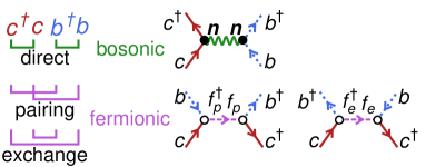
The direct channel involves the mean-fields and , which represent the magnetic moments of the itinerant electron and the spinon, respectively. Here the Hund’s rule coupling term is decomposed into (omiting the band and site indices)
| (6) |
By integrating out the itinerant electron and the spinon degrees of freedom, and will acquire dynamics, behaving like a collective magnon mode which describes the magnetic fluctuations. Denoting the magnon propagator by a wavy line
![]() , then it can be depicted by the following Feynman diagrams
, then it can be depicted by the following Feynman diagrams
The pairing channel involves a mean-field , which can be considered as a composite fermion as a bound state of the itinerant electron with the bosonic spinon. In this channel, the mean-field decomposition takes the following form
| (7) |
Similarly the exchange channel takes a mean-field , which can be regarded as a composite fermion bound state of the itinerant electron and anti-spinon. In this channel, the mean-field decomposition takes the following form
| (8) |
By integrating out the itinerant electron and the spinon degrees of freedom, and will acquire their dynamics, which behave as composite fermions. Denoting the composite fermion propagator by a dashed line
![]() , the emergence of such a composite fermion can be depicted by the following Feynman diagrams
, the emergence of such a composite fermion can be depicted by the following Feynman diagrams
As a combination of the itinerant electron and the spinon, such composite fermions represent a unique collective charge mode in the two-fluid model whose physical consequence will be discussed later.
II.3 Mean-Field Phase Diagram
The SDW and the SC phases are the most prominent phases in the phase diagram of iron-based compounds. They can be understood qualitatively from the mean-field theory of the two-fluid model.
Let us start with the SDW phase, in which the magnetism is neither fully itinerant nor fully local origin.Johannes and Mazin (2009) Based on the hybrid theory,Kou et al. (2009); You et al. (2011a) the SDW phase is the consequence of a joint effort of the coupled itinerant and localized degrees of freedom. Due to the Hund’s rule coupling, the SDW ordering of the itinerant electrons, , provides an effective “Zeeman-like” field to the spinons, which polarizes the spinons along the same spin directions. In return, a spinon magnetic ordering will act back on the itinerant electrons, helping to stabilize the SDW ordering. The itinerant electron and the local moment will thus mutually polarize each other, as described by the mean-field decomposition in Eq. (6). Such a positive feedback will lead to the simultaneous ordering of both the itinerant electron and the local moment SDW order parameters and . Combined with the itinerant electron and the spinon band structures, the mean field solution of and can be determined self-consistently,You and Weng (2013) as shown in Fig. 6(a).

As the doping level increases, the nesting instability of the itinerant electron Fermi surface is suppressed.Kou et al. (2009); You et al. (2011a); You and Weng (2013) Without the SDW ordering, the local moments will remain in a spin liquid state. The gapped para-magnon excitation in the spin liquid state will nevertheless drive a Cooper pairing instability of the itinerant electrons. Here the magnon plays the same roleScalapino et al. (1986) as the phonon in a conventional superconductor. Thus, in the two-fluid model, the iron-based superconductor is basically still a BCS superconductor with the charge carrieres provided by the itinerant electrons and the pairing glue by the local moment fluctuations.
In a magnon-gluon BCS theory,You et al. (2011a); You and Weng (2013) there exists a cutoff frequency of magnons (similar to the Debey frequency of phonons). The SC transition temperature is controlled by this energy scale . Comparing with the phonon, the magnon cutoff frequency can be higher by one order of magnitude, which explains why the iron-based superconductor can support a relatively high . In the singlet channel, the magnon mediates a repulsive interaction.Kou et al. (2009); You et al. (2011a); You and Weng (2013) Thus the Fermi pockets at and points, connected by the magnon momentum (i.e. the magnetic ordering momentum) should take the opposite pairing sign, leading to the -wave pairing symmetry similar to the itinerant theoryMazin and Schmalian (2009); Parish et al. (2008); Ummarino et al. (2009) Fig. 6(b) shows the mean field calculation of the SC order parameters in the electron doped case.You and Weng (2013)
Putting the SDW and SC together, a mean-field phase diagram can be mapped out, as shown in Fig. 7. With increasing doping, the SDW transition line may end at a tricritical point that can further split into first order transitions.Chubukov et al. (2008); Chubukov (2009); You et al. (2011b) The coexistence/competition of the SDW and SC order in the intermediate phase has also been discussed in Ref. Vorontsov et al., 2009, 2010.

In summary, the overall phase diagram of the iron-based compound may be qualitatively understood in the hybrid/two-fluid picture. Here in both the SDW and the SC phases, the coexistence of the itinerant electrons and the local moments are crucial to the underlying mechanisms. In the SDW phase, the itinerant electrons and the local moments mutually interact to facilitate a joint ordering, while in the SC phase, the itinerant charge carriers are paired via the gluon provided by the local moment fluctuations.
II.4 Spin Dynamics
II.4.1 NMR Knight Shift
The two-fluid behavior is also reflected in the NMR Knight shift. The Knight shift basically measures the uniform spin susceptibility as a function of temperature, which includes the contributions from both the itinerant electron and the local moment . At the RPA level, one finds
| (9) |
where is the effective Hund’s rule coupling strength. For a Fermi liquid, follows the Pauli susceptibility behavior, which is almost independent of . For a spin liquid, follows a linear- behavior as shown before.Kou et al. (2009); You et al. (2011b). Since and are much smaller compared to , the denominator in Eq. (9) is not important, which is simplified to . Its typical behavior is shown in Fig. 8, together with and .

At higher temperatures, the spin liquid (local moment) dominates the linear- behavior, while the Fermi liquid behavior takes over as the temperature lowers, where the Knight shift would saturate to a constant Pauli susceptibility. However, further taking into account of the SDW transition, the Fermi liquid susceptibility will suddenly be reduced below the transition temperature (see Fig. 8), as the Fermi surface density of states gets depleted due to the SDW gap opening. The coexistence of the high-temperature linear- behavior and the low-temperature SDW gap-opening behavior in a single curve of the Knight shiftImai et al. (2009); Ma et al. (2011); Michioka et al. (2010); Nakai et al. (2009); Ning et al. (2009, 2010) once again supports the two-fluid description.
II.4.2 INS Spectrum
The two-fluid character is manifested not only in the static spin response, but also in the dynamic spin fluctuations. The INS experiment can probe the dynamic spin-spin correlation , which again includes the contributions from both the itinerant, , and local moment, , degrees of freedom at the RPA level:
| (10) |
with being the frequency-momentum vector. While the dynamic spectral function of the local moments, described by , is not much affected in different phases, the contribution from the itinerant electrons, , is quite sensitive to different states of the itinerant electrons, as shown in Fig. 9(a,c,e).
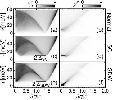
In the normal state, the dynamic spin susceptibility of the Fermi liquid simply forms a Stoner continuum as in Fig. 9(a). The total dynamic spin susceptibility measured by INS spectrum shows a massive dispersion relation of the local moment magnon Fig. 9(b), with the certain degree of blurring due to the self-energy correction brought by the Stoner continuum of the itinerant electron.
In the SC phase, the Stoner continuum is gapped up by the SC gap as in Fig. 9(c). The discontinuity of at the gap edge leads to the divergence of according to the Kramer-Kronig relation. Then from Eq. (10), the denominator could easily vanish given enough coupling strength , leading to the divergence of . This gives rise to the spin-resonance at the energy scale of around the magnetic ordering momentum in the SC phase, as shown in Fig. 9(d), a phenomenon that has been observedArgyriou et al. (2010); Chi et al. (2009); Christianson et al. (2008); Christianson et al. (2009); Harriger et al. (2012); Inosov et al. (2010); Li et al. (2009b); Lumsden et al. (2009); Lumsden and Christianson (2010); Lynn and Dai (2009); Qiu et al. (2009); Seo et al. (2009); Taylor et al. (2011); Wang et al. (2012); Wen et al. (2010); Xu et al. (2011) in various families of iron-based superconductors.
In the SDW phase, the Stoner continuum of the itinerant electron is gaped up by the SDW gap , as shown in Fig. 9(e). Due to the broken spin rotational symmetry in the SDW phase, the spin fluctuations can be divided into the transverse fluctuation (perpendicular to the magnetization direction) and the longitudinal fluctuation (parallel to the magnetization). For the transverse fluctuation, a gapless Goldstone mode will emerge inside the SDW gap shown in Fig. 9(f), as the new poles of . The gapless Goldstone mode is a consequence of the spontaneous broken spin-rotation symmetry in forming the SDW joint ordering. While for the longitudinal fluctuation, the magnon mode will remain gapped. The gap of the longitudinal mode is about , which is related to the spin fluctuation asscociated with the itinerant electron, since a minimal energy is required to excite an SDW electron-hole pair as the longitudinal mode. Thus, a low-energy longitudinal spin fluctuation observed in the SDW phase is an evidence for the presence of the itinerant magnetism.
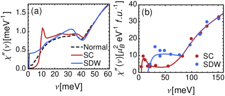
Therefore, the spin fluctuations have been studiedYou and Weng (2013) as an RPA combination from the two-fluid components. The low-energy spin fluctuations are much affected by states of the itinerant electron, which behaves differently in different phases. On the other hand, the high-energy spin fluctuations mainly reflect the dynamics of the local moment, which is much less sensitive to either SDW or SC ordering. The low- and high-energy sectors are separated by the upper edge, a kink structure, of the Stoner continuum of the itinerant electron, illustrated in Fig. 10(a). Such behavior is consistent with the experiments,Argyriou et al. (2010); Liu et al. (2012) as shown in Fig. 10(b). Moreover, at the low energies, the RPA correction naturally gives rise to a spin-resonance mode in the SC phase as well as a Goldstone mode (spin wave excitation) in the SDW phase.
II.5 Charge Dynamics
II.5.1 Resistivity
The transport property of the iron-based compound is determined by the itinerant electron near the Fermi surface, which basically follows the Fermi liquid behavior. The scattering of the itinerant electron with the underlying local moment fluctuation provides an important source of dissipation. The self-energy correct of the itinerant electron due to the electron-spinon scattering can be evaluated on the RPA level.You et al. (2011a) At low temperature and small frequency , it was shownYou et al. (2011a) that the imaginary part of the self-energy approximately follows the or behavior (depending on which one is greater). This gives rise to the dependence of the resistivity at low temperature, typical for the Fermi liquid.
In the SDW phase, such a behavior of the resistivity is in competition with the thermal activation behavior across the SDW gap. As temperature increases, the SDW gap is suppressed, and more itinerant electrons are thermally excited across the SDW gap to contribute to the conductivity. So this activation effect tends to reduce the resistivity with the temperature, which is in opposite to the behavior. The competition between these two factors may eventually lead to a hump in the resistivity curve for under-doped compounds in the SDW phase, as the curve in Fig. 1.
According to the Kramers-Kronig relation, the real part of the self-energy should follow the behavior, which leads to the band renormalization effect. As has been reported in various ARPES experiments,Lu et al. (2008); Liu et al. (2008); Yang et al. (2009); Lu et al. (2009); Xia et al. (2009); Liu et al. (2009); Borisenko et al. (2010); Cui et al. (2012) all pockets are shallower than the bare band structure predicted by the DFT calculationsCao et al. (2008); Singh and Du (2008); Mazin et al. (2008); Kuroki et al. (2008); Deng et al. (2009); Graser et al. (2010) The mass enhancement factor can be as strong as 2 to 3.Anisimov et al. (2009); Ferber et al. (2012)
II.5.2 STM Spectrum
The STM differential conductance ( spectrum) basically measures the electron local density of states. The STM studiesMassee et al. (2010); Zhou et al. (2012); Wang et al. (2013) in many iron-based superconductors have discovered a hump-dip feature in the normal phase, as shown in Fig. 11. Starting from the low temperature SC phase and raising the temperature into the normal phase, an hump-dip feature was leftover around the Fermi level in the normal state after the closure of the SC gap (at around 20K for NaFe0.94Co0.06As and 40K for Ba0.6K0.4Fe2As2), see Fig. 11. It was also found that the dip structure is locked to the Fermi surface under different doping with asymmetric line shape. Moreover, from the electron-doped Fig. 11(a) to the hole-doped Fig. 11(b) compounds, the spectrum is particle-hole reflected about the Fermi level.
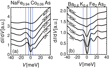
Given the observed facts, this hump-dip structure can be explained neither as an SDW gap due to its locking with the Fermi level, nor as a SC gap due to the asymmetric line shape. One possible explanation is that the hump structure represents a charge resonance mode, originated from the composite fermion discussed in the above two-fluid model. Due to the effective Hund’s rule interaction between the itinerant electron and the spinon, they may be bound together into a composite fermion, which carries one electron charge and an integer spin. For an intermediate coupling strength, the composite fermion mode will emerge near the Fermi surface within the spin gap. In a finite doping, the electron spectrum is particle-hole asymmetric, so is the composite fermion mode about the Fermi level. It is foundYou and Weng (2013) that the composite fermion mode will emerge from below the Fermi energy for the electron-doping, and from above the Fermi energy for the hole-doping. If we regard the hump structure in the STM spectrum as the signal of the composite fermion mode, then the asymmetric line shape and the doping dependence can both be understood consistently as below.You and Weng (2013)
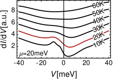
In Fig. 12, the composite fermion mode is reflected in the spectrum via the inelastic electron tunneling.Hahn et al. (2000) If the electron from the STM tip tunnels into the sample with an energy higher than that of the composite fermion, new tunneling channels will be opened up, leading to the hump structure in the spectrum. The hump appears at the energy scale of the composite fermion mode, which is locked to the Fermi level by the spin gap. The calculation is done for the electron-doped case. For the hole-doped case, the spectrum will simply reversed with respect to the Fermi level, which is consistent with the experimental observations.
III Summary
In the present Chapter, we presented a minimal, phenomenological description of the low-energy physics in the iron-based superconductors. The general framework and physical consequences are summarized in Fig. 13 from the viewpoint of renormalization group.
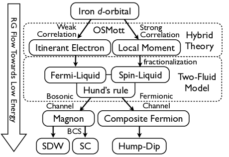
Strarting from the iron orbital electrons, their microscopic dynamics may be described by a multi-band Hubbard model Eq. (1). Due to the multi-band and intermediate correlation characters, an orbital-selective Mott transition becomes possible. Under an RG flow, the difference among different electron bands may be amplified, which then leads to distinct RG fixed points. Some bands flow to the strong correlation fixed point of the local moments, while the others flow to the weak correlation fixed point of the itinerant electrons. The itinerant electrons and the local moments can thus coexist in the system in the RG sense, coupled together via a residual Hund’s rule interaction. This constitutes the basic rationale for the hybrid theory in Eq. (3).
At a lower temperature, the itinerant electrons form a Fermi liquid, characterized by well-defined quasi-particles around the Fermi pockets, which can further experience typical Fermi-liquid instabilities such as SDW and SC. On the other hand, the local moments remain disordered due to strong quantum fluctuations, which may be modeled by a spin liquid with fractionalized bosonic spinons by a two-fluid model [Eq. (4)].
In the two-fluid model, the Fermi liquid of the itinerant electron and the spin liquid of the local moment are coupled together by a residual Hund’s rule coupling, which may be treated perturbatively in a weak or intermediate coupling strength. There are two types of low-lying collective modes arising from this coupled two-fluid model.
In the bosonic channel, a magnon-like excitation as a bound state of the spinons reflects the strong magnetic correlations of the local moments. It couples to the itinerant electrons to induce an SDW ordering of the latter, while simulaneously lead to a CAMF ordering of the local moments in the magnetic phase of the iron-based superconductor. On the other hand, the magnon-mediated effective pairing between the itinerant electrons competes with the SDW ordering near the Fermi surfaces, resulting in an SC state in proper parameter regimes.
A unique prediction of the two-fluid model is that besides the usual quasiparticle excitation, a new composite fermion mode may emerge as a bound state of the itinerant electron and the local moment under an intermediate Hund’s rule interaction. It carries the same charge as an itinerant electron but with a different spin quantum number, which participates in the low energy charge transport and leads to the hump-dip structure observed in the STM inelastic electron tunneling spectrum (IETS) in the iron-based compounds.
Finally, we point out that the iron-based superconductor is not the only known physics system that may possess the coexisting itinerant electrons and local moments. The heavy fermion systemAndres et al. (1975); Steglich et al. (1979) discovered in the 1970’s is already one of such examples. The theoretical framework Nakatsuji et al. (2004); Yang and Pines (2008); Yang et al. (2008) at low energy also contains two fluid components: the Fermi liquid of the coherent electrons and the Kondo lattice, in which the local moment at each site couples to the itinerant electron via the antiferromagnetic Kondo interaction. Such Kondo lattice model looks similar to the hybrid model of the iron-based superconductor. One of main distinctions lies in whether the coupling described by the term is antiferromagnetic (Kondo) or ferromagnetic (Hund’s rule). But this difference is important. The RG equation is sensitive to the sign of the coupling : the Kondo coupling can flow to infinity towards low energy, while the Hund’s rule coupling flows to zero. So in some sense, the iron-based superconductor system is simpler comparing to the heavy fermion system because the Hund’s rule coupling can be treated perturbatively. Even in the single-band - model, via the fractionalization, a two-fluid description of the spin correlations has been recently proposed in the superconducting state, where the Mott localized spins and doping-induced hopping effect are described by a two-component RVB structure in the ground state wave function.
Acknowledgements.
Previous collaborations and discussions with S.P. Kou, F. Yang, Y.Y. Wang, and T. Li related to the present work are acknowledged. This work was supported by the NBRPC grant no. 2010CB923003.References
- Haule et al. (2008) K. Haule, J. H. Shim, and G. Kotliar, Physical Review Letters 100, 226402 (2008), URL http://link.aps.org/doi/10.1103/PhysRevLett.100.226402.
- Ma and Lu (2008) F. Ma and Z.-Y. Lu, Physical Review B 78, 033111 (2008), URL http://link.aps.org/doi/10.1103/PhysRevB.78.033111.
- Kuroki et al. (2008) K. Kuroki, S. Onari, R. Arita, H. Usui, Y. Tanaka, H. Kontani, and H. Aoki, Physical Review Letters 101, 087004 (2008), URL http://link.aps.org/doi/10.1103/PhysRevLett.101.087004.
- Singh (2008) D. J. Singh, Physical Review B 78, 094511 (2008), URL http://link.aps.org/doi/10.1103/PhysRevB.78.094511.
- Subedi et al. (2008) A. Subedi, L. Zhang, D. J. Singh, and M. H. Du, Physical Review B 78, 134514 (2008), URL http://link.aps.org/doi/10.1103/PhysRevB.78.134514.
- Bardeen et al. (1957a) J. Bardeen, L. N. Cooper, and J. R. Schrieffer, Physical Review 106, 162 (1957a), URL http://link.aps.org/doi/10.1103/PhysRev.106.162.
- Bardeen et al. (1957b) J. Bardeen, L. N. Cooper, and J. R. Schrieffer, Physical Review 108, 1175 (1957b), URL http://link.aps.org/doi/10.1103/PhysRev.108.1175.
- Anderson (1987) P. W. Anderson, Science 235, 1196 (1987).
- Anderson et al. (2004) P. W. Anderson, P. A. Lee, M. Randeria, T. M. Rice, N. Trivedi, and F. C. Zhang, Journal of Physics Condensed Matter 16, 755 (2004), eprint arXiv:cond-mat/0311467.
- Bardeen and Pines (1955) J. Bardeen and D. Pines, Physical Review 99, 1140 (1955), URL http://link.aps.org/doi/10.1103/PhysRev.99.1140.
- Kohn and Luttinger (1965) W. Kohn and J. M. Luttinger, Physical Review Letters 15, 524 (1965), URL http://link.aps.org/doi/10.1103/PhysRevLett.15.524.
- Berk and Schrieffer (1966) N. F. Berk and J. R. Schrieffer, Physical Review Letters 17, 433 (1966), URL http://link.aps.org/doi/10.1103/PhysRevLett.17.433.
- Doniach and Engelsberg (1966) S. Doniach and S. Engelsberg, Physical Review Letters 17, 750 (1966), URL http://link.aps.org/doi/10.1103/PhysRevLett.17.750.
- Bickers and Scalapino (1989) N. E. Bickers and D. J. Scalapino, Annals of Physics 193, 206 (1989), URL http://www.sciencedirect.com/science/article/pii/000349168990359X.
- Shankar (1994) R. Shankar, Reviews of Modern Physics 66, 129 (1994), URL http://link.aps.org/doi/10.1103/RevModPhys.66.129.
- Qazilbash et al. (2009) M. M. Qazilbash, J. J. Hamlin, R. E. Baumbach, L. Zhang, D. J. Singh, M. B. Maple, and D. N. Basov, Nature Physics 5, 647 (2009), eprint 0909.0312.
- Johnston (2010) D. Johnston, Advances in Physics 59, 803 (2010), eprint 1005.4392.
- Kou et al. (2009) S.-P. Kou, T. Li, and Z.-Y. Weng, Europhysics Letters 88, 17010 (2009), URL http://stacks.iop.org/0295-5075/88/i=1/a=17010.
- Kamihara et al. (2008) Y. Kamihara, T. Watanabe, M. Hirano, and H. Hosono, J. Am. Chem. Soc. 130, 3296 (2008).
- Ren et al. (2008a) Z.-A. Ren, W. Lu, J. Yang, W. Yi, X.-L. Shen, Z.-C. Li, G.-C. Che, X.-L. Dong, L.-L. Sun, F. Zhou, et al., Chinese Physics Letters 25, 2215 (2008a).
- Ren et al. (2008b) Z.-A. Ren, J. Yang, W. Lu, W. Yi, X.-L. Shen, Z.-C. Li, G.-C. Che, X.-L. Dong, L.-L. Sun, F. Zhou, et al., Europhysics Letters 82, 57002 (2008b), URL http://stacks.iop.org/0295-5075/82/i=5/a=57002.
- Chen et al. (2008a) X. H. Chen, T. Wu, G. Wu, R. H. Liu, H. Chen, and D. F. Fang, Nature 453, 761 (2008a).
- Kito et al. (2008) H. Kito, H. Eisaki, and A. Iyo, Journal of the Physical Society of Japan 77, 063707 (2008), URL http://jpsj.ipap.jp/link?JPSJ/77/063707/.
- Tapp et al. (2008) J. H. Tapp, Z. Tang, B. Lv, K. Sasmal, B. Lorenz, P. C. W. Chu, and A. M. Guloy, Physical Review B 78, 060505 (2008), URL http://link.aps.org/doi/10.1103/PhysRevB.78.060505.
- Sefat et al. (2008) A. S. Sefat, R. Jin, M. A. McGuire, B. C. Sales, D. J. Singh, and D. Mandrus, Physical Review Letters 101, 117004 (2008), URL http://link.aps.org/doi/10.1103/PhysRevLett.101.117004.
- Rotter et al. (2008) M. Rotter, M. Tegel, and D. Johrendt, Physical Review Letters 101, 107006 (2008), URL http://link.aps.org/doi/10.1103/PhysRevLett.101.107006.
- Wang et al. (2008) X. C. Wang, Q. Q. Liu, Y. X. Lv, W. B. Gao, L. X. Yang, R. C. Yu, F. Y. Li, and C. Q. Jin, Solid State Communications 148, 538 (2008), eprint 0806.4688.
- Wang et al. (2008) C. Wang, L. Li, S. Chi, Z. Zhu, Z. Ren, Y. Li, Y. Wang, X. Lin, Y. Luo, S. Jiang, et al., Europhysics Letters 83, 67006 (2008), URL http://stacks.iop.org/0295-5075/83/i=6/a=67006.
- Sales et al. (2009) B. C. Sales, A. S. Sefat, M. A. McGuire, R. Y. Jin, D. Mandrus, and Y. Mozharivskyj, Physical Review B 79, 094521 (2009), URL http://link.aps.org/doi/10.1103/PhysRevB.79.094521.
- Chen et al. (2009) G. F. Chen, W. Z. Hu, J. L. Luo, and N. L. Wang, Physical Review Letters 102, 227004 (2009), URL http://link.aps.org/doi/10.1103/PhysRevLett.102.227004.
- Chu et al. (2009) C. W. Chu, F. Chen, M. Gooch, A. M. Guloy, B. Lorenz, B. Lv, K. Sasmal, Z. J. Tang, J. H. Tapp, and Y. Y. Xue, Physica C: Superconductivity 469, 326 (2009), URL http://www.sciencedirect.com/science/article/pii/S0921453409000653.
- Fang et al. (2009) L. Fang, H. Luo, P. Cheng, Z. Wang, Y. Jia, G. Mu, B. Shen, I. I. Mazin, L. Shan, C. Ren, et al., Physical Review B 80, 140508 (2009), URL http://link.aps.org/doi/10.1103/PhysRevB.80.140508.
- Si and Abrahams (2008) Q. Si and E. Abrahams, Physical Review Letters 101, 076401 (2008), URL http://link.aps.org/doi/10.1103/PhysRevLett.101.076401.
- Singh and Du (2008) D. J. Singh and M. H. Du, Physical Review Letters 100, 237003 (2008), URL http://link.aps.org/doi/10.1103/PhysRevLett.100.237003.
- Cao et al. (2008) C. Cao, P. J. Hirschfeld, and H.-P. Cheng, Physical Review B 77, 220506 (2008), URL http://link.aps.org/doi/10.1103/PhysRevB.77.220506.
- Liu et al. (2008) C. Liu, G. D. Samolyuk, Y. Lee, N. Ni, T. Kondo, A. F. Santander-Syro, S. L. Bud’ko, J. L. McChesney, E. Rotenberg, T. Valla, et al., Physical Review Letters 101, 177005 (2008), URL http://link.aps.org/doi/10.1103/PhysRevLett.101.177005.
- Lu et al. (2009) D. H. Lu, M. Yi, S. K. Mo, J. G. Analytis, J. H. Chu, A. S. Erickson, D. J. Singh, Z. Hussain, T. H. Geballe, I. R. Fisher, et al., Physica C: Superconductivity 469, 452 (2009), URL http://www.sciencedirect.com/science/article/pii/S092145340900080X.
- Cui et al. (2012) S. T. Cui, S. Y. Zhu, A. F. Wang, S. Kong, S. L. Ju, X. G. Luo, X. H. Chen, G. B. Zhang, and Z. Sun, Physical Review B 86, 155143 (2012), URL http://link.aps.org/doi/10.1103/PhysRevB.86.155143.
- Vilmercati et al. (2009) P. Vilmercati, A. Fedorov, I. Vobornik, U. Manju, G. Panaccione, A. Goldoni, A. S. Sefat, M. A. McGuire, B. C. Sales, R. Jin, et al., Physical Review B 79, 220503 (2009), URL http://link.aps.org/doi/10.1103/PhysRevB.79.220503.
- Xia et al. (2009) Y. Xia, D. Qian, L. Wray, D. Hsieh, G. F. Chen, J. L. Luo, N. L. Wang, and M. Z. Hasan, Physical Review Letters 103, 037002 (2009), URL http://link.aps.org/doi/10.1103/PhysRevLett.103.037002.
- Borisenko et al. (2010) S. V. Borisenko, V. B. Zabolotnyy, D. V. Evtushinsky, T. K. Kim, I. V. Morozov, A. N. Yaresko, A. A. Kordyuk, G. Behr, A. Vasiliev, R. Follath, et al., Physical Review Letters 105, 067002 (2010), URL http://link.aps.org/doi/10.1103/PhysRevLett.105.067002.
- He et al. (2010) C. He, Y. Zhang, B. P. Xie, X. F. Wang, L. X. Yang, B. Zhou, F. Chen, M. Arita, K. Shimada, H. Namatame, et al., Physical Review Letters 105, 117002 (2010), URL http://link.aps.org/doi/10.1103/PhysRevLett.105.117002.
- Aichhorn et al. (2009) M. Aichhorn, L. Pourovskii, V. Vildosola, M. Ferrero, O. Parcollet, T. Miyake, A. Georges, and S. Biermann, Physical Review B 80, 085101 (2009), URL http://link.aps.org/doi/10.1103/PhysRevB.80.085101.
- Coldea et al. (2008) A. I. Coldea, J. D. Fletcher, A. Carrington, J. G. Analytis, A. F. Bangura, J. H. Chu, A. S. Erickson, I. R. Fisher, N. E. Hussey, and R. D. McDonald, Physical Review Letters 101, 216402 (2008), URL http://link.aps.org/doi/10.1103/PhysRevLett.101.216402.
- Sebastian et al. (2008) S. E. Sebastian, J. Gillett, N. Harrison, P. H. C. Lau, D. J. Singh, C. H. Mielke, and G. G. Lonzarich, Journal of Physics: Condensed Matter 20, 422203 (2008), URL http://stacks.iop.org/0953-8984/20/i=42/a=422203.
- Coldea et al. (2009) A. I. Coldea, C. M. J. Andrew, J. G. Analytis, R. D. McDonald, A. F. Bangura, J. H. Chu, I. R. Fisher, and A. Carrington, Physical Review Letters 103, 026404 (2009), URL http://link.aps.org/doi/10.1103/PhysRevLett.103.026404.
- Analytis et al. (2009a) J. G. Analytis, C. M. J. Andrew, A. I. Coldea, A. McCollam, J. H. Chu, R. D. McDonald, I. R. Fisher, and A. Carrington, Physical Review Letters 103, 076401 (2009a), URL http://link.aps.org/doi/10.1103/PhysRevLett.103.076401.
- Analytis et al. (2009b) J. G. Analytis, R. D. McDonald, J.-H. Chu, S. C. Riggs, A. F. Bangura, C. Kucharczyk, M. Johannes, and I. R. Fisher, Physical Review B 80, 064507 (2009b), URL http://link.aps.org/doi/10.1103/PhysRevB.80.064507.
- Ran et al. (2009) Y. Ran, F. Wang, H. Zhai, A. Vishwanath, and D.-H. Lee, Physical Review B 79, 014505 (2009), URL http://link.aps.org/doi/10.1103/PhysRevB.79.014505.
- Zhou et al. (2012) X. Zhou, P. Cai, A. Wang, W. Ruan, C. Ye, X. Chen, Y. You, Z.-Y. Weng, and Y. Wang, Physical Review Letters 109, 037002 (2012), URL http://link.aps.org/doi/10.1103/PhysRevLett.109.037002.
- Hu et al. (2008) W. Z. Hu, J. Dong, G. Li, Z. Li, P. Zheng, G. F. Chen, J. L. Luo, and N. L. Wang, Physical Review Letters 101, 257005 (2008), URL http://link.aps.org/doi/10.1103/PhysRevLett.101.257005.
- Moon and Choi (2010) C.-Y. Moon and H. J. Choi, Physical Review Letters 104, 057003 (2010), URL http://link.aps.org/doi/10.1103/PhysRevLett.104.057003.
- Moon et al. (2010) S. J. Moon, J. H. Shin, D. Parker, W. S. Choi, I. I. Mazin, Y. S. Lee, J. Y. Kim, N. H. Sung, B. K. Cho, S. H. Khim, et al., Physical Review B 81, 205114 (2010), URL http://link.aps.org/doi/10.1103/PhysRevB.81.205114.
- Wang et al. (2012) N. L. Wang, W. Z. Hu, Z. G. Chen, R. H. Yuan, G. Li, G. F. Chen, and T. Xiang, Journal of Physics Condensed Matter 24, C4202 (2012), eprint 1105.3939.
- de La Cruz et al. (2008) C. de La Cruz, Q. Huang, J. W. Lynn, J. Li, W. R. , II, J. L. Zarestky, H. A. Mook, G. F. Chen, J. L. Luo, N. L. Wang, et al., Nature 453, 899 (2008), eprint 0804.0795.
- Chen et al. (2008b) Y. Chen, J. W. Lynn, J. Li, G. Li, G. F. Chen, J. L. Luo, N. L. Wang, P. Dai, C. dela Cruz, and H. A. Mook, Physical Review B 78, 064515 (2008b), URL http://link.aps.org/doi/10.1103/PhysRevB.78.064515.
- Kimber et al. (2008) S. A. J. Kimber, D. N. Argyriou, F. Yokaichiya, K. Habicht, S. Gerischer, T. Hansen, T. Chatterji, R. Klingeler, C. Hess, G. Behr, et al., Physical Review B 78, 140503 (2008), URL http://link.aps.org/doi/10.1103/PhysRevB.78.140503.
- Qiu et al. (2008) Y. Qiu, W. Bao, Q. Huang, T. Yildirim, J. M. Simmons, M. A. Green, J. W. Lynn, Y. C. Gasparovic, J. Li, T. Wu, et al., Physical Review Letters 101, 257002 (2008), URL http://link.aps.org/doi/10.1103/PhysRevLett.101.257002.
- Zhao et al. (2008a) J. Zhao, Q. Huang, C. de la Cruz, S. Li, J. W. Lynn, Y. Chen, M. A. Green, G. F. Chen, G. Li, Z. Li, et al., Nature Materials 7, 953 (2008a), URL http://dx.doi.org/10.1038/nmat2315.
- Xiao et al. (2009a) Y. Xiao, Y. Su, R. Mittal, T. Chatterji, T. Hansen, C. M. N. Kumar, S. Matsuishi, H. Hosono, and T. Brueckel, Physical Review B 79, 060504 (2009a), URL http://link.aps.org/doi/10.1103/PhysRevB.79.060504.
- Xiao et al. (2010) Y. Xiao, Y. Su, R. Mittal, T. Chatterji, T. Hansen, S. Price, C. M. N. Kumar, J. Persson, S. Matsuishi, Y. Inoue, et al., Physical Review B 81, 094523 (2010), URL http://link.aps.org/doi/10.1103/PhysRevB.81.094523.
- Tian et al. (2010) W. Tian, I. Ratcliff, W., M. G. Kim, J. Q. Yan, P. A. Kienzle, Q. Huang, B. Jensen, K. W. Dennis, R. W. McCallum, T. A. Lograsso, et al., Physical Review B 82, 060514 (2010), URL http://link.aps.org/doi/10.1103/PhysRevB.82.060514.
- Goldman et al. (2008) A. I. Goldman, D. N. Argyriou, B. Ouladdiaf, T. Chatterji, A. Kreyssig, S. Nandi, N. Ni, S. L. Bud’ko, P. C. Canfield, and R. J. McQueeney, Physical Review B 78, 100506 (2008), URL http://link.aps.org/doi/10.1103/PhysRevB.78.100506.
- Zhao et al. (2008b) J. Zhao, I. Ratcliff, W., J. W. Lynn, G. F. Chen, J. L. Luo, N. L. Wang, J. Hu, and P. Dai, Physical Review B 78, 140504 (2008b), URL http://link.aps.org/doi/10.1103/PhysRevB.78.140504.
- Kaneko et al. (2008) K. Kaneko, A. Hoser, N. Caroca-Canales, A. Jesche, C. Krellner, O. Stockert, and C. Geibel, Physical Review B 78, 212502 (2008), URL http://link.aps.org/doi/10.1103/PhysRevB.78.212502.
- Huang et al. (2008) Q. Huang, Y. Qiu, W. Bao, M. A. Green, J. W. Lynn, Y. C. Gasparovic, T. Wu, G. Wu, and X. H. Chen, Physical Review Letters 101, 257003 (2008), URL http://link.aps.org/doi/10.1103/PhysRevLett.101.257003.
- Matan et al. (2009) K. Matan, R. Morinaga, K. Iida, and T. J. Sato, Physical Review B 79, 054526 (2009), URL http://link.aps.org/doi/10.1103/PhysRevB.79.054526.
- Wilson et al. (2009) S. D. Wilson, Z. Yamani, C. R. Rotundu, B. Freelon, E. Bourret-Courchesne, and R. J. Birgeneau, Physical Review B 79, 184519 (2009), URL http://link.aps.org/doi/10.1103/PhysRevB.79.184519.
- Xiao et al. (2009b) Y. Xiao, Y. Su, M. Meven, R. Mittal, C. M. N. Kumar, T. Chatterji, S. Price, J. Persson, N. Kumar, S. K. Dhar, et al., Physical Review B 80, 174424 (2009b), URL http://link.aps.org/doi/10.1103/PhysRevB.80.174424.
- Li et al. (2009a) S. Li, C. de la Cruz, Q. Huang, Y. Chen, J. W. Lynn, J. Hu, Y.-L. Huang, F.-C. Hsu, K.-W. Yeh, M.-K. Wu, et al., Physical Review B 79, 054503 (2009a), URL http://link.aps.org/doi/10.1103/PhysRevB.79.054503.
- Bao et al. (2009) W. Bao, Y. Qiu, Q. Huang, M. A. Green, P. Zajdel, M. R. Fitzsimmons, M. Zhernenkov, S. Chang, M. Fang, B. Qian, et al., Physical Review Letters 102, 247001 (2009), URL http://link.aps.org/doi/10.1103/PhysRevLett.102.247001.
- Martinelli et al. (2010) A. Martinelli, A. Palenzona, M. Tropeano, C. Ferdeghini, M. Putti, M. R. Cimberle, T. D. Nguyen, M. Affronte, and C. Ritter, Physical Review B 81, 094115 (2010), URL http://link.aps.org/doi/10.1103/PhysRevB.81.094115.
- Liu et al. (2010) T. J. Liu, J. Hu, B. Qian, D. Fobes, Z. Q. Mao, W. Bao, M. Reehuis, S. A. J. Kimber, K. Prokeš, S. Matas, et al., Nature Materials 9, 718 (2010), URL http://dx.doi.org/10.1038/nmat2800.
- Rodriguez and Rezayi (2009) J. P. Rodriguez and E. H. Rezayi, Physical Review Letters 103, 097204 (2009), URL http://link.aps.org/doi/10.1103/PhysRevLett.103.097204.
- Hansmann et al. (2010) P. Hansmann, R. Arita, A. Toschi, S. Sakai, G. Sangiovanni, and K. Held, Physical Review Letters 104, 197002 (2010), URL http://link.aps.org/doi/10.1103/PhysRevLett.104.197002.
- Gretarsson et al. (2011) H. Gretarsson, A. Lupascu, J. Kim, D. Casa, T. Gog, W. Wu, S. R. Julian, Z. J. Xu, J. S. Wen, G. D. Gu, et al., Physical Review B 84, 100509 (2011), URL http://link.aps.org/doi/10.1103/PhysRevB.84.100509.
- Vilmercati et al. (2012) P. Vilmercati, A. Fedorov, F. Bondino, F. Offi, G. Panaccione, P. Lacovig, L. Simonelli, M. A. McGuire, A. S. M. Sefat, D. Mandrus, et al., Physical Review B 85, 220503 (2012), URL http://link.aps.org/doi/10.1103/PhysRevB.85.220503.
- Bonville et al. (2010) P. Bonville, F. Rullier-Albenque, D. Colson, and A. Forget, Europhysics Letters 89, 67008 (2010), URL http://stacks.iop.org/0295-5075/89/i=6/a=67008.
- Zhao et al. (2009) J. Zhao, D. T. Adroja, D.-X. Yao, R. Bewley, S. Li, X. F. Wang, G. Wu, X. H. Chen, J. Hu, and P. Dai, Nature Physics 5, 555 (2009), URL http://dx.doi.org/10.1038/nphys1336.
- Xu et al. (2011) Z. Xu, J. Wen, G. Xu, S. Chi, W. Ku, G. Gu, and J. M. Tranquada, Physical Review B 84, 052506 (2011), URL http://link.aps.org/doi/10.1103/PhysRevB.84.052506.
- Ning et al. (2009) F. Ning, K. Ahilan, T. Imai, A. S. Sefat, R. Jin, M. A. McGuire, B. C. Sales, and D. Mandrus, Journal of the Physical Society of Japan 78, 013711 (2009), eprint 0811.1617.
- Imai et al. (2009) T. Imai, K. Ahilan, F. L. Ning, T. M. McQueen, and R. J. Cava, Physical Review Letters 102, 177005 (2009), URL http://link.aps.org/doi/10.1103/PhysRevLett.102.177005.
- Ning et al. (2010) F. L. Ning, K. Ahilan, T. Imai, A. S. Sefat, M. A. McGuire, B. C. Sales, D. Mandrus, P. Cheng, B. Shen, and H. H. Wen, Physical Review Letters 104, 037001 (2010), URL http://link.aps.org/doi/10.1103/PhysRevLett.104.037001.
- Michioka et al. (2010) C. Michioka, H. Ohta, M. Matsui, J. Yang, K. Yoshimura, and M. Fang, Physical Review B 82, 064506 (2010), URL http://link.aps.org/doi/10.1103/PhysRevB.82.064506.
- Ma et al. (2011) L. Ma, G. F. Ji, J. Dai, J. B. He, D. M. Wang, G. F. Chen, B. Normand, and W. Yu, Physical Review B 84, 220505 (2011), eprint 1103.4960.
- Yan et al. (2008) J. Q. Yan, A. Kreyssig, S. Nandi, N. Ni, S. L. Bud’ko, A. Kracher, R. J. McQueeney, R. W. McCallum, T. A. Lograsso, A. I. Goldman, et al., Physical Review B 78, 024516 (2008), URL http://link.aps.org/doi/10.1103/PhysRevB.78.024516.
- Wu et al. (2008) G. Wu, H. Chen, T. Wu, Y. L. Xie, Y. J. Yan, R. H. Liu, X. F. Wang, J. J. Ying, and X. H. Chen, Journal of Physics: Condensed Matter 20, 422201 (2008), URL http://stacks.iop.org/0953-8984/20/i=42/a=422201.
- Wang et al. (2009a) X. F. Wang, T. Wu, G. Wu, H. Chen, Y. L. Xie, J. J. Ying, Y. J. Yan, R. H. Liu, and X. H. Chen, Physical Review Letters 102, 117005 (2009a), URL http://link.aps.org/doi/10.1103/PhysRevLett.102.117005.
- Klingeler et al. (2010) R. Klingeler, N. Leps, I. Hellmann, A. Popa, U. Stockert, C. Hess, V. Kataev, H. J. Grafe, F. Hammerath, G. Lang, et al., Physical Review B 81, 024506 (2010), URL http://link.aps.org/doi/10.1103/PhysRevB.81.024506.
- Zhang et al. (2009) G. M. Zhang, Y. H. Su, Z. Y. Lu, Z. Y. Weng, D. H. Lee, and T. Xiang, Europhysics Letters 86, 37006 (2009), eprint 0809.3874.
- Mazin et al. (2008) I. I. Mazin, D. J. Singh, M. D. Johannes, and M. H. Du, Physical Review Letters 101, 057003 (2008), URL http://link.aps.org/doi/10.1103/PhysRevLett.101.057003.
- Yildirim (2008) T. Yildirim, Physical Review Letters 101, 057010 (2008), URL http://link.aps.org/doi/10.1103/PhysRevLett.101.057010.
- Chubukov et al. (2008) A. V. Chubukov, D. V. Efremov, and I. Eremin, Physical Review B 78, 134512 (2008), URL http://link.aps.org/doi/10.1103/PhysRevB.78.134512.
- Sknepnek et al. (2009) R. Sknepnek, G. Samolyuk, Y.-B. Lee, and J. Schmalian, Physical Review B 79, 054511 (2009), URL http://link.aps.org/doi/10.1103/PhysRevB.79.054511.
- Maier et al. (2009) T. A. Maier, S. Graser, D. J. Scalapino, and P. J. Hirschfeld, Physical Review B 79, 224510 (2009), URL http://link.aps.org/doi/10.1103/PhysRevB.79.224510.
- Wang et al. (2009b) F. Wang, H. Zhai, Y. Ran, A. Vishwanath, and D.-H. Lee, Physical Review Letters 102, 047005 (2009b), URL http://link.aps.org/doi/10.1103/PhysRevLett.102.047005.
- Zhai et al. (2009) H. Zhai, F. Wang, and D.-H. Lee, Physical Review B 80, 064517 (2009), URL http://link.aps.org/doi/10.1103/PhysRevB.80.064517.
- Ummarino et al. (2009) G. A. Ummarino, M. Tortello, D. Daghero, and R. S. Gonnelli, Physical Review B 80, 172503 (2009), URL http://link.aps.org/doi/10.1103/PhysRevB.80.172503.
- Seo et al. (2008) K. Seo, B. A. Bernevig, and J. Hu, Physical Review Letters 101, 206404 (2008), URL http://link.aps.org/doi/10.1103/PhysRevLett.101.206404.
- Craco et al. (2008) L. Craco, M. S. Laad, S. Leoni, and H. Rosner, Physical Review B 78, 134511 (2008), URL http://link.aps.org/doi/10.1103/PhysRevB.78.134511.
- Haule and Kotliar (2009) K. Haule and G. Kotliar, New Journal of Physics 11, 025021 (2009), URL http://stacks.iop.org/1367-2630/11/i=2/a=025021.
- Laad et al. (2009) M. S. Laad, L. Craco, S. Leoni, and H. Rosner, Physical Review B 79, 024515 (2009), URL http://link.aps.org/doi/10.1103/PhysRevB.79.024515.
- Abrahams and Si (2011) E. Abrahams and Q. Si, Journal of Physics: Condensed Matter 23, 223201 (2011), URL http://stacks.iop.org/0953-8984/23/i=22/a=223201.
- Hu and Ding (2012) J. Hu and H. Ding, Nature Scientific Reports 2, 381 (2012), eprint 1107.1334.
- Yu and Si (2012) R. Yu and Q. Si, Physical Review B 86, 085104 (2012), URL http://link.aps.org/doi/10.1103/PhysRevB.86.085104.
- Flint and Coleman (2012) R. Flint and P. Coleman, Physical Review B 86, 184508 (2012), URL http://link.aps.org/doi/10.1103/PhysRevB.86.184508.
- Weng (2009) Z.-Y. Weng, Physica E: Low-dimensional Systems and Nanostructures 41, 1281 (2009), URL http://www.sciencedirect.com/science/article/pii/S1386947709000538.
- Yin et al. (2010) W.-G. Yin, C.-C. Lee, and W. Ku, Physical Review Letters 105, 107004 (2010), URL http://link.aps.org/doi/10.1103/PhysRevLett.105.107004.
- Lv et al. (2010) W. Lv, F. Krüger, and P. Phillips, Physical Review B 82, 045125 (2010), URL http://link.aps.org/doi/10.1103/PhysRevB.82.045125.
- Gor’kov and Teitel’baum (2013) L. P. Gor’kov and G. B. Teitel’baum, Physical Review B 87, 024504 (2013), URL http://link.aps.org/doi/10.1103/PhysRevB.87.024504.
- Raghu et al. (2008) S. Raghu, X.-L. Qi, C.-X. Liu, D. J. Scalapino, and S.-C. Zhang, Physical Review B 77, 220503 (2008), URL http://link.aps.org/doi/10.1103/PhysRevB.77.220503.
- Lee and Wen (2008) P. A. Lee and X.-G. Wen, Physical Review B 78, 144517 (2008), URL http://link.aps.org/doi/10.1103/PhysRevB.78.144517.
- Scalapino et al. (1986) D. J. Scalapino, J. Loh, E., and J. E. Hirsch, Physical Review B 34, 8190 (1986), URL http://link.aps.org/doi/10.1103/PhysRevB.34.8190.
- Pines (1997a) D. Pines, Zeitschrift fur Physik B Condensed Matter 103, 129 (1997a), eprint arXiv:cond-mat/9702187.
- Pines (1997b) D. Pines, Physica C Superconductivity 282, 273 (1997b), eprint arXiv:cond-mat/9704102.
- Yu et al. (2009) S.-L. Yu, J. Kang, and J.-X. Li, Physical Review B 79, 064517 (2009), URL http://link.aps.org/doi/10.1103/PhysRevB.79.064517.
- Yao et al. (2009) Z.-J. Yao, J.-X. Li, and Z. D. Wang, New Journal of Physics 11, 025009 (2009), URL http://stacks.iop.org/1367-2630/11/i=2/a=025009.
- Chubukov (2009) A. V. Chubukov, Physica C Superconductivity 469, 640 (2009), eprint 0902.4188.
- Vorontsov et al. (2009) A. B. Vorontsov, M. G. Vavilov, and A. V. Chubukov, Physical Review B 79, 060508 (2009), URL http://link.aps.org/doi/10.1103/PhysRevB.79.060508.
- Vorontsov et al. (2010) A. B. Vorontsov, M. G. Vavilov, and A. V. Chubukov, Physical Review B 81, 174538 (2010), URL http://link.aps.org/doi/10.1103/PhysRevB.81.174538.
- Fernandes and Schmalian (2010) R. M. Fernandes and J. Schmalian, Phys. Rev. B 82, 014521 (2010), URL http://link.aps.org/doi/10.1103/PhysRevB.82.014521.
- Arita and Ikeda (2009) R. Arita and H. Ikeda, Journal of the Physical Society of Japan 78, 113707 (2009), eprint arXiv:0909.1413.
- Si et al. (2009) Q. Si, E. Abrahams, J. Dai, and J.-X. Zhu, New Journal of Physics 11, 045001 (2009), URL http://stacks.iop.org/1367-2630/11/i=4/a=045001.
- Mazin and Schmalian (2009) I. I. Mazin and J. Schmalian, Physica C: Superconductivity 469, 614 (2009), URL http://www.sciencedirect.com/science/article/pii/S0921453409001002.
- Gutzwiller (1963) M. C. Gutzwiller, Physical Review Letters 10, 159 (1963), URL http://link.aps.org/doi/10.1103/PhysRevLett.10.159.
- Hubbard (1963) J. Hubbard, Proceedings of the Royal Society of London. Series A. Mathematical and Physical Sciences 276, 238 (1963).
- Georges et al. (1996) A. Georges, G. Kotliar, W. Krauth, and M. J. Rozenberg, Reviews of Modern Physics 68, 13 (1996), URL http://link.aps.org/doi/10.1103/RevModPhys.68.13.
- de’Medici et al. (2009) L. de’Medici, S. R. Hassan, M. Capone, and X. Dai, Physical Review Letters 102, 126401 (2009), URL http://link.aps.org/doi/10.1103/PhysRevLett.102.126401.
- Hackl and Vojta (2009) A. Hackl and M. Vojta, New Journal of Physics 11, 055064 (2009), eprint 0812.3394.
- Vojta (2010) M. Vojta, Journal of Low Temperature Physics 161, 203 (2010), eprint 1006.1559.
- de’Medici (2011) L. de’Medici, Physical Review B 83, 205112 (2011), URL http://link.aps.org/doi/10.1103/PhysRevB.83.205112.
- Yu and Si (2011) R. Yu and Q. Si, Physical Review B 84, 235115 (2011), URL http://link.aps.org/doi/10.1103/PhysRevB.84.235115.
- Zhang et al. (2012) Y.-Z. Zhang, H. Lee, H.-Q. Lin, C.-Q. Wu, H. O. Jeschke, and R. Valentí, Physical Review B 85, 035123 (2012), URL http://link.aps.org/doi/10.1103/PhysRevB.85.035123.
- Quan et al. (2012) Y. M. Quan, L. J. Zou, D. Y. Liu, and H. Q. Lin, The European Physical Journal B 85, 1 (2012), URL http://dx.doi.org/10.1140/epjb/e2011-20613-0.
- Yu and Si (2012) R. Yu and Q. Si, arXiv:1208.5547 (2012), eprint 1208.5547.
- Johannes and Mazin (2009) M. D. Johannes and I. I. Mazin, Physical Review B 79, 220510 (2009), URL http://link.aps.org/doi/10.1103/PhysRevB.79.220510.
- Wang et al. (2010) G. Wang, Y. Qian, G. Xu, X. Dai, and Z. Fang, Physical Review Letters 104, 047002 (2010), URL http://link.aps.org/doi/10.1103/PhysRevLett.104.047002.
- You et al. (2011a) Y.-Z. You, F. Yang, S.-P. Kou, and Z.-Y. Weng, Physical Review B 84, 054527 (2011a), URL http://link.aps.org/doi/10.1103/PhysRevB.84.054527.
- Tisza (1938) L. Tisza, Nature 141, 913 (1938).
- Arovas and Auerbach (1988) D. P. Arovas and A. Auerbach, Physical Review B 38, 316 (1988), URL http://link.aps.org/doi/10.1103/PhysRevB.38.316.
- Wen (1991) X. G. Wen, Physical Review B 44, 2664 (1991), URL http://link.aps.org/doi/10.1103/PhysRevB.44.2664.
- Sachdev and Read (1991) S. Sachdev and N. Read, International Journal of Modern Physics B 5, 219 (1991), eprint arXiv:cond-mat/0402109.
- Read and Sachdev (1991) N. Read and S. Sachdev, Physical Review Letters 66, 1773 (1991), URL http://link.aps.org/doi/10.1103/PhysRevLett.66.1773.
- Chubukov et al. (1994) A. V. Chubukov, T. Senthil, and S. Sachdev, Physical Review Letters 72, 2089 (1994), URL http://link.aps.org/doi/10.1103/PhysRevLett.72.2089.
- Senthil et al. (2004) T. Senthil, L. Balents, S. Sachdev, A. Vishwanath, and M. P. A. Fisher, Physical Review B 70, 144407 (2004), URL http://link.aps.org/doi/10.1103/PhysRevB.70.144407.
- Yao et al. (2010) H. Yao, L. Fu, and X.-L. Qi, arXiv:1012.4470 (2010), eprint 1012.4470.
- You and Weng (2013) Y.-Z. You and Z.-Y. Weng, ArXiv e-prints (2013), eprint 1306.3740.
- Parish et al. (2008) M. M. Parish, J. Hu, and B. A. Bernevig, Physical Review B 78, 144514 (2008), URL http://link.aps.org/doi/10.1103/PhysRevB.78.144514.
- You et al. (2011b) Y.-Z. You, F. Yang, S.-P. Kou, and Z.-Y. Weng, Physical Review Letters 107, 167001 (2011b), URL http://link.aps.org/doi/10.1103/PhysRevLett.107.167001.
- Nakai et al. (2009) Y. Nakai, S. Kitagawa, K. Ishida, Y. Kamihara, M. Hirano, and H. Hosono, Journal of Physics: Conference Series 150, 052179 (2009), URL http://stacks.iop.org/1742-6596/150/i=5/a=052179.
- Argyriou et al. (2010) D. N. Argyriou, A. Hiess, A. Akbari, I. Eremin, M. M. Korshunov, J. Hu, B. Qian, Z. Mao, Y. Qiu, C. Broholm, et al., Physical Review B 81, 220503 (2010), URL http://link.aps.org/doi/10.1103/PhysRevB.81.220503.
- Chi et al. (2009) S. Chi, A. Schneidewind, J. Zhao, L. W. Harriger, L. Li, Y. Luo, G. Cao, Z. Xu, M. Loewenhaupt, J. Hu, et al., Physical Review Letters 102, 107006 (2009), URL http://link.aps.org/doi/10.1103/PhysRevLett.102.107006.
- Christianson et al. (2008) A. D. Christianson, E. A. Goremychkin, R. Osborn, S. Rosenkranz, M. D. Lumsden, C. D. Malliakas, I. S. Todorov, H. Claus, D. Y. Chung, M. G. Kanatzidis, et al., Nature 456, 930 (2008).
- Christianson et al. (2009) A. D. Christianson, M. D. Lumsden, S. E. Nagler, G. J. MacDougall, M. A. McGuire, A. S. Sefat, R. Jin, B. C. Sales, and D. Mandrus, Physical Review Letters 103, 087002 (2009), URL http://link.aps.org/doi/10.1103/PhysRevLett.103.087002.
- Harriger et al. (2012) L. W. Harriger, O. J. Lipscombe, C. Zhang, H. Luo, M. Wang, K. Marty, M. D. Lumsden, and P. Dai, Physical Review B 85, 054511 (2012), URL http://link.aps.org/doi/10.1103/PhysRevB.85.054511.
- Inosov et al. (2010) D. S. Inosov, J. T. Park, P. Bourges, D. L. Sun, Y. Sidis, A. Schneidewind, K. Hradil, D. Haug, C. T. Lin, B. Keimer, et al., Nature Physics 6, 178 (2010), URL http://dx.doi.org/10.1038/nphys1483.
- Li et al. (2009b) S. Li, Y. Chen, S. Chang, J. W. Lynn, L. Li, Y. Luo, G. Cao, Z. Xu, and P. Dai, Physical Review B 79, 174527 (2009b), URL http://link.aps.org/doi/10.1103/PhysRevB.79.174527.
- Lumsden et al. (2009) M. D. Lumsden, A. D. Christianson, D. Parshall, M. B. Stone, S. E. Nagler, G. J. MacDougall, H. A. Mook, K. Lokshin, T. Egami, D. L. Abernathy, et al., Physical Review Letters 102, 107005 (2009), URL http://link.aps.org/doi/10.1103/PhysRevLett.102.107005.
- Lumsden and Christianson (2010) M. D. Lumsden and A. D. Christianson, Journal of Physics: Condensed Matter 22, 203203 (2010), URL http://stacks.iop.org/0953-8984/22/i=20/a=203203.
- Lynn and Dai (2009) J. W. Lynn and P. Dai, Physica C: Superconductivity 469, 469 (2009), URL http://www.sciencedirect.com/science/article/pii/S0921453409000823.
- Qiu et al. (2009) Y. Qiu, W. Bao, Y. Zhao, C. Broholm, V. Stanev, Z. Tesanovic, Y. C. Gasparovic, S. Chang, J. Hu, B. Qian, et al., Physical Review Letters 103, 067008 (2009), URL http://link.aps.org/doi/10.1103/PhysRevLett.103.067008.
- Seo et al. (2009) K. Seo, C. Fang, B. A. Bernevig, and J. Hu, Physical Review B 79, 235207 (2009), URL http://link.aps.org/doi/10.1103/PhysRevB.79.235207.
- Taylor et al. (2011) A. E. Taylor, M. J. Pitcher, R. A. Ewings, T. G. Perring, S. J. Clarke, and A. T. Boothroyd, Physical Review B 83, 220514 (2011), URL http://link.aps.org/doi/10.1103/PhysRevB.83.220514.
- Wang et al. (2012) M. Wang, C. Li, D. L. Abernathy, Y. Song, S. V. Carr, X. Lu, S. Li, Z. Yamani, J. Hu, T. Xiang, et al., Physical Review B 86, 024502 (2012), URL http://link.aps.org/doi/10.1103/PhysRevB.86.024502.
- Wen et al. (2010) J. Wen, G. Xu, Z. Xu, Z. W. Lin, Q. Li, Y. Chen, S. Chi, G. Gu, and J. M. Tranquada, Physical Review B 81, 100513 (2010), URL http://link.aps.org/doi/10.1103/PhysRevB.81.100513.
- Liu et al. (2012) M. Liu, L. W. Harriger, H. Luo, M. Wang, R. A. Ewings, T. Guidi, H. Park, K. Haule, G. Kotliar, S. M. Hayden, et al., Nature Physics 8, 376 (2012), eprint 1202.2827.
- Lu et al. (2008) D. H. Lu, M. Yi, S.-K. Mo, A. S. Erickson, J. Analytis, J.-H. Chu, D. J. Singh, Z. Hussain, T. H. Geballe, I. R. Fisher, et al., Nature 455, 81 (2008), eprint 0807.2009.
- Yang et al. (2009) L. X. Yang, Y. Zhang, H. W. Ou, J. F. Zhao, D. W. Shen, B. Zhou, J. Wei, F. Chen, M. Xu, C. He, et al., Physical Review Letters 102, 107002 (2009).
- Liu et al. (2009) G. Liu, H. Liu, L. Zhao, W. Zhang, X. Jia, J. Meng, X. Dong, J. Zhang, G. F. Chen, G. Wang, et al., Physical Review B 80, 134519 (2009), URL http://link.aps.org/doi/10.1103/PhysRevB.80.134519.
- Deng et al. (2009) S. Deng, J. Köhler, and A. Simon, Physical Review B 80, 214508 (2009), URL http://link.aps.org/doi/10.1103/PhysRevB.80.214508.
- Graser et al. (2010) S. Graser, A. F. Kemper, T. A. Maier, H. P. Cheng, P. J. Hirschfeld, and D. J. Scalapino, Physical Review B 81, 214503 (2010), URL http://link.aps.org/doi/10.1103/PhysRevB.81.214503.
- Anisimov et al. (2009) V. I. Anisimov, E. Z. Kurmaev, A. Moewes, and I. A. Izyumov, Physica C Superconductivity 469, 442 (2009), eprint 0905.3038.
- Ferber et al. (2012) J. Ferber, K. Foyevtsova, R. Valentí, and H. O. Jeschke, Physical Review B 85, 094505 (2012), URL http://link.aps.org/doi/10.1103/PhysRevB.85.094505.
- Massee et al. (2010) F. Massee, Y. K. Huang, J. Kaas, E. van Heumen, S. de Jong, R. Huisman, H. Luigjes, J. B. Goedkoop, and M. S. Golden, Europhysics Letters 92, 57012 (2010), URL http://stacks.iop.org/0295-5075/92/i=5/a=57012.
- Wang et al. (2013) Z. Wang, H. Yang, D. Fang, B. Shen, Q.-H. Wang, L. Shan, C. Zhang, P. Dai, and H.-H. Wen, Nature Physics 9, 42 (2013).
- Hahn et al. (2000) J. R. Hahn, H. J. Lee, and W. Ho, Physical Review Letters 85, 1914 (2000), URL http://link.aps.org/doi/10.1103/PhysRevLett.85.1914.
- Andres et al. (1975) K. Andres, J. E. Graebner, and H. R. Ott, Physical Review Letters 35, 1779 (1975), URL http://link.aps.org/doi/10.1103/PhysRevLett.35.1779.
- Steglich et al. (1979) F. Steglich, J. Aarts, C. D. Bredl, W. Lieke, D. Meschede, W. Franz, and H. Schäfer, Physical Review Letters 43, 1892 (1979), URL http://link.aps.org/doi/10.1103/PhysRevLett.43.1892.
- Nakatsuji et al. (2004) S. Nakatsuji, D. Pines, and Z. Fisk, Physical Review Letters 92, 016401 (2004), URL http://link.aps.org/doi/10.1103/PhysRevLett.92.016401.
- Yang and Pines (2008) Y.-f. Yang and D. Pines, Physical Review Letters 100, 096404 (2008), URL http://link.aps.org/doi/10.1103/PhysRevLett.100.096404.
- Yang et al. (2008) Y.-f. Yang, Z. Fisk, H.-O. Lee, J. D. Thompson, and D. Pines, Nature 454, 611 (2008), URL http://dx.doi.org/10.1038/nature07157.