A Portable Parton-Level Event Generator for the High-Luminosity LHC

Enrico Bothmann^1$\star$, Taylor Childers², Walter Giele³, Stefan Höche³, Joshua Isaacson³ and Max Knobbe¹

Abstract

The rapid deployment of computing hardware different from the traditional CPU+RAM model in data centers around the world mandates a change in the design of event generators for the Large Hadron Collider, in order to provide economically and ecologically sustainable simulations for the high-luminosity era of the LHC. Parton-level event generation is one of the most computationally demanding parts of the simulation and is therefore a prime target for improvements. We present the first complete leading-order parton-level event generation framework capable of utilizing most modern hardware and discuss its performance in the standard candle processes of vector boson and top-quark pair production with up to five additional jets.

Copyright attribution to authors.
This work is a submission to SciPost Physics.
License information to appear upon publication.
Publication information to appear upon publication. Received Date
Accepted Date
Published Date

 

Contents

1. 1 Introduction
2. 2 Basic algorithms
   1. 2.1 Tree-level amplitudes
   2. 2.2 Phase-space integration
3. 3 Event generation framework
   1. 3.1 Summation of partonic channels
   2. 3.2 Helicity integration
   3. 3.3 Event data layout and parallel event generation
   4. 3.4 Portability solutions
   5. 3.5 Event output
4. 4 Validation
5. 5 Performance
   1. 5.1 Baseline CPU performance
   2. 5.2 Performance on different hardware
   3. 5.3 Scaling to many nodes
6. 6 Summary and Outlook
7. A Tabulated performance results
8. B Runtime distribution

 

1 Introduction

Monte-Carlo simulations of detector events are a cornerstone of high-energy physics [1, 2]. Simulated events are usually fully differential in momentum and flavor space, such that the same analysis pipeline can be used for both the experimental data and the theoretical prediction. This methodology has enabled precise tests of the Standard Model and searches for theories beyond it. Traditionally, the computing performance of event simulations has been of relatively little importance, due to the far greater demands of the subsequent detector simulation. However, the high luminosity of the LHC and the excellent understanding of the ATLAS and CMS detectors call for ever more precise calculations. This is rapidly leading to a situation where poor performance of event simulations can become a limiting factor for the success of experimental analyses [3, 4]. In addition, the impact of LHC computing on climate change must be considered, and its carbon footprint be kept as low as reasonably achievable [5].

Alleviating this problem has been a focus of interest recently. Tremendous improvements of existing code bases have been obtained from improved event generation algorithms and PDF interpolation routines [6, 7]. Phase-space integrators have been equipped with adaptive algorithms based on neural networks [8, 9, 10, 11, 12, 13] and updated with simple, yet efficient analytic solutions [14]. Negative weights in NLO matching procedures were reduced systematically [15, 16], and analytic calculations have been used to replace numerical methods when available [17]. Neural network based methods have been devised to construct surrogate matrix elements with improved numerical performance [18, 19, 20, 21]. All those developments have in common that they operate on well-established code bases for the computation of matrix elements in the traditional CPU+RAM model. At the same time, the deployment of heterogeneous computing systems is steadily accelerated by the increasing need to provide platforms for AI software. This presents a formidable challenge to the high-energy physics community, with its rigid code structures and slow-paced development, caused by a persistent lack of human resources. The Generator Working Group of the HEP Software Foundation and the HEP Center for Computational Excellence have therefore both identified the construction of portable simulation programs as essential for the success of the high-luminosity LHC. Some exploratory work was performed in [22, 23, 24, 25], and first concrete steps towards a generic solution have been reported in [26, 27, 28, 29, 30].

In this manuscript we will describe the hardware agnostic implementation of a complete leading-order parton-level event generator for processes that are simulated at high statistical precision at the LHC, including $Z/\gamma+$jets, $t\bar{t}+$jets, pure jets and multiple heavy quark production. The most significant obstacle in these computations is the low unweighting efficiency at high particle multiplicity, combined with exponential scaling (in the best case) of the integrand [31]. We demonstrate that new algorithms and widely available modern hardware alleviate this problem to a degree that renders previously highly challenging computations accessible for everyday analyses. We make the code base available for public use and provide an interface to a recently completed particle-level event simulation framework [32], enabling state-of-the art collider phenomenology with our new generator.

This manuscript is organized as follows. Section 2 recalls the main results of previous studies on matrix-element and phase-space generation and details the extension to a production-level code base. Section 3 introduces our new simulation framework, which we call Pepper , and discusses the techniques for managing partonic sub-processes, helicity integration, projection onto leading-color configurations, and other aspects relevant for practical applications. Section 5 is focused on the computing performance of the new framework, both in comparison to existing numerical simulations and in comparison between different hardware. Section 6 presents possible future directions of development.

2 Basic algorithms

The computation of tree-level matrix elements and the generation of phase-space points are the components with the largest footprint in state-of-the-art LHC simulations [31, 7]. We aim to reduce their evaluation time as much as possible, while also focusing on simplicity, portability and scalability of the implementation. Reference [26] presented a dedicated study to find the best algorithms for the computation of all-gluon amplitudes on GPUs. Here we extend the method to processes including quarks. We also recall the results of Ref. [14], which presented an efficient concept for phase-space integration easily extensible to GPUs. We make a few simple changes in the algorithm, which lead to a large increase in efficiency without complicating the structure of the code or impairing portability.

2.1 Tree-level amplitudes

We use the all-gluon process often discussed in the literature as an example to introduce the basic concepts of matrix-element computation. A color and spin summed squared $n$-gluon tree-level amplitude is defined as

$$|\mathcal{A}(1,\ldots,n)|^{2}=\sum_{a_{1}\ldots a_{n}}\mathcal{A}_{a_{1}\ldots a_{n}}^{\mu_{1}\cdots\mu_{n}}(p_{1},\ldots,p_{n})\left(\mathcal{A}_{a_{1}\ldots a_{n}}^{\nu_{1}\cdots\nu_{n}}(p_{1},\ldots,p_{n})\right)^{\dagger}\prod_{i=1}^{n}\sum_{\lambda_{i}}\epsilon_{\mu_{i}}^{\lambda_{i}}(p,k)\epsilon_{\nu_{i}}^{\lambda_{i}\,\dagger}(p,k)\;,$$ (1)

where each gluon with label $i$ is characterized by its momentum $p_{i}$, its color $a_{i}$ and its helicity $\lambda_{i}=\pm$. The squared $n$-gluon amplitude then takes the form

$$|\mathcal{A}(1,\ldots,n)|^{2}=\sum_{\lambda_{1}\ldots\lambda_{n}}\sum_{a_{1}\ldots a_{n}}\mathcal{A}_{a_{1}\ldots a_{n}}^{\lambda_{1}\ldots\lambda_{n}}(p_{1},\ldots,p_{n})\left(\mathcal{A}_{a_{1}\ldots a_{n}}^{\lambda_{1}\ldots\lambda_{n}}(p_{1},\ldots,p_{n})\right)^{\dagger}\;,$$ (2)

where the $\mathcal{A}^{\lambda}$ are the chirality-dependent scattering amplitudes obtained by contracting $\mathcal{A}^{\mu}$ with the helicity eigenstates $\epsilon_{\mu}^{\lambda}$ of the external gluons. The treatment of color in this calculation is a complex problem. The most promising approach for LHC physics at low to medium jet multiplicity is to explicitly sum over color states using a color-decomposition with a minimal basis [26]. In the pure gluon case, this basis is given by the adjoint representation [33, 34, 35]

$$\mathcal{A}_{a_{1}\ldots a_{n}}^{\lambda_{1}\ldots\lambda_{n}}(p_{1},\ldots,p_{n})=\sum\limits_{\vec{\sigma}\in S_{n-2}}(F^{a_{\sigma_{2}}}\ldots F^{a_{\sigma_{n-1}}})_{a_{1}a_{n}}\;A^{\lambda_{1}\ldots\lambda_{n}}(p_{1},p_{\sigma_{2}},\ldots,p_{\sigma_{n-1}},p_{n})\;,$$ (3)

where $F^{a}_{bc}=if^{abc}$ and $f^{abc}$ are the ${\rm SU}(3)$ structure constants. The functions $A$ are called color-ordered or partial amplitudes and are stripped of all color information, which is now contained entirely in the prefactor. If the amplitudes carry helicity labels, they are often also referred to as helicity amplitudes. The multi-index $\vec{\sigma}$ runs over all permutations $S_{n-2}$ of the ($n-2$) gluon indices $2,\ldots,n-1$. The color basis thus defined is minimal and has $(n-2)!$ elements.

For amplitudes involving not only gluons but also quarks, the minimal color basis is given in terms of Dyck words [36, 37]. A Dyck word is a set of opening and closing brackets, such that the number of opening brackets is always larger or equal to the number of closing ones for any subset starting at the beginning of the Dyck word. For example for four characters and one type of bracket, there are two Dyck words, $(())$ and $()()$. In the context of QCD amplitude computations, every opening bracket represents a quark and every closing one an anti-quark. Different types of brackets can appear and indicate differently flavored quarks. Similar to the gluon case in Eq. (3), one may keep two parton indices fixed throughout the computation and permute all others, as long as the permutation forms a valid Dyck word. The number of partial amplitudes in this basis is minimal. For $n$ particles and $k$ distinct quark pairs, it is given by $(n-2)!/k!$, which is a generalization of the minimal all-gluon ($k=0$) result. The color factors needed for the computations can be evaluated using the algorithm described in [38, 39].

There are various algorithms to compute the partial amplitudes $A(p_{1},\ldots,p_{n})$ in Eq. (3) (we now omit helicity labels for brevity). The numerical efficiency of the most promising approaches has been compared in [40, 41, 42, 26]. It was found that, for generic helicity configurations and arbitrary particle multiplicity, the Berends–Giele recursive relations [43, 44, 45] offer the best performance. We therefore choose this method for our new matrix-element generator. The basic objects in the Berends–Giele approach are off-shell currents, $J(1,\ldots,n)$. In the case of an all-gluon amplitude, they are defined as

$$\begin{split}&J_{\mu}(1,2,\ldots,n)=\frac{-ig_{\mu\nu}}{p_{1,n}^{2}}\bigg{\{}\;\vphantom{\sum_{k=j+1}^{n-1}}\sum_{k=1}^{n-1}V_{3}^{\nu\kappa\lambda}(p_{1,k},p_{k+1,n})J_{\kappa}(1,\ldots,k)J_{\lambda}(k+1,\ldots,n)\\ &\qquad\qquad+\sum_{j=1}^{n-2}\sum_{k=j+1}^{n-1}V_{4}^{\nu\rho\kappa\lambda}J_{\rho}(1,\ldots,j)J_{\kappa}(j+1,\ldots,k)J_{\lambda}(k+1,\ldots,n)\bigg{\}}\;,\end{split}$$ (4)

where the $p_{i}$ denote the momenta of the gluons, $p_{i,j}=p_{i}+\ldots+p_{j}$ and $V_{3}^{\nu\kappa\lambda}$ and $V_{4}^{\nu\rho\kappa\lambda}$ are the color-ordered three- and four-gluon vertices:

$$\begin{split}V_{3}^{\nu\kappa\lambda}(p,q)&=i\,\frac{g_{s}}{\sqrt{2}}\big{(}\,g^{\kappa\lambda}(p-q)^{\nu}+g^{\lambda\nu}(2q+p)^{\kappa}-g^{\nu\kappa}(2p+q)^{\lambda}\,\big{)}\;,\\ V_{4}^{\nu\rho\kappa\lambda}&=i\,\frac{g_{s}^{2}}{2}\big{(}\,2g^{\nu\kappa}g^{\rho\lambda}-g^{\nu\rho}g^{\kappa\lambda}-g^{\nu\lambda}g^{\rho\kappa}\,\big{)}\;.\end{split}$$ (5)

The external particle currents, $J_{\mu}(i)$, are given by the helicity eigenstates, $\epsilon_{\mu}(p_{i})$. The complete amplitude $A(p_{1},\ldots,p_{n})$ is obtained by putting the ($n-1$)-particle off-shell current $J_{\mu}(1,\ldots,n-1)$ on-shell and contracting it with the external polarization $J_{\mu}(n)$:

$$A(p_{1},\ldots,p_{n})=J_{\mu}(n)\,p_{1,n}^{2}\,J^{\mu}(1,\ldots,n-1)\;.$$ (6)

A major advantage of this formulation of the calculation is that it can straightforwardly be extended to processes including massless and massive quarks, as well as to calculations involving non-QCD particles. The external currents for fermions are given by spinors, and the three- and four-particle vertices are fully determined by the Standard Model interactions.

2.2 Phase-space integration

The differential phase space element for an $n$-particle final state at a hadron collider with fixed incoming momenta $p_{a}$ and $p_{b}$ and outgoing momenta $\{p_{1},\ldots,p_{n}\}$ is given by [46]

$${\rm d}\Phi_{n}(a,b;1,\ldots,n)=\left[\,\prod\limits_{i=1}^{n}\frac{{\rm d}^{3}\vec{p}_{i}}{(2\pi)^{3}\,2E_{i}}\,\right]\,(2\pi)^{4}\delta^{(4)}\bigg{(}p_{a}+p_{b}-\sum_{i=1}^{n}p_{i}\bigg{)}\;.$$ (7)

For processes without $s$-channel resonances, it is convenient to parameterize Eq. (7) by

$$\begin{split}{\rm d}x_{a}{\rm d}x_{b}\,{\rm d}\Phi_{n}(a,b;1,\ldots,n)=&\;\frac{2\pi}{s}\left[\,\prod_{i=1}^{n-1}\frac{1}{16\pi^{2}}\,{\rm d}p_{i,\perp}^{2}\,{\rm d}y_{i}\,\frac{\rm d\phi_{i}}{2\pi}\,\right]\,{\rm d}y_{n}\;,\end{split}$$ (8)

where, $p_{i,\perp}$, $y_{i}$ and $\phi_{i}$ are the transverse momentum, rapidity and azimuthal angle of momentum $i$ in the laboratory frame, and where $x_{a}$ and $x_{b}$ are the Bjørken variables of the incoming partons. In processes with unambiguous $s$-channel topologies, such as Drell–Yan lepton pair production, one may instead use the strategy of [14] and parameterize the decay of the resonance using the well-known two-body decay formula

$${\rm d}\Phi_{2}(\{1,2\};1,2)=\frac{1}{16\pi^{2}}\frac{\sqrt{(p_{1}p_{2})^{2}-p_{1}^{2}p_{2}^{2}}}{(p_{1}+p_{2})^{2}}\,{\rm d}\cos\theta_{1}^{\{1,2\}}\,{\rm d}\phi_{1}^{\{1,2\}}\;,$$ (9)

which, as written here, has been evaluated in the center-of-mass frame of the decaying particle. The $t$- and $s$-channel building blocks in Eqs. (8) and (9) can be combined using the standard factorization formula [47]

$${\rm d}\Phi_{n}(a,b;1,\ldots,n)={\rm d}\Phi_{n-m+1}(a,b;\{1,..,m\},m+1,\ldots,n)\,\frac{{\rm d}s_{\{1,..,m\}}}{2\pi}\,{\rm d}\Phi_{m}(\{1,..,m\};1,\ldots,m)\;.$$ (10)

We will refer to this minimal integration technique as the basic Chili method. It is both simple to implement, and reasonably efficient due to the compact form of the compute kernels [14]. The latter aspect is especially important in the context of code portability and maintenance.

Compared to the first implementation in Ref. [14], we apply two improvements which increase the integration efficiency significantly: 1) In the azimuthal angle integration of Eq. (8), the sum of previously generated momenta serves to define $\phi=0$. 2) Assuming that particles $1$ through $m$ are subject to transverse momentum cuts, and assuming $n$ final-state particles overall, we generate the transverse momenta of the $n-m$ particles not subject to cuts according to a peaked distribution given by $1/(p_{i,\perp}+p_{\perp,0})$, where $p_{\perp,0}=|\sum_{i=1}^{m}\vec{p}_{i,\perp}|/(n-m)$. We also use $\sum_{i=1}^{m}\vec{p}_{i,\perp}$ to define $\phi=0$ for the corresponding azimuthal angle integration.

3 Event generation framework

The construction of a production-ready matrix element generator requires many design choices beyond the basic matrix element and phase space calculation routines discussed in Sec. 2. In most experimental analyses, flavors are not resolved inside jets, and the sum over partons can be performed with the help of symmetries among the QCD amplitudes. In addition, an efficient strategy must be found to perform helicity sums. For a parallelized code such as Pepper, two additional questions must be addressed: how to arrange the event data for efficient calculations on massively parallel architectures, and how to write the generated parton-level events to persistent storage without unnecessarily limiting the data transfer rate. We will discuss these aspects in the following.

3.1 Summation of partonic channels

In the Pepper event generator, the partonic processes which contribute to the hadronic cross section are arranged into groups, such that all processes within a group have the same partonic matrix element. For any given phase-space point, the matrix element squared is evaluated only once, and then multiplied by the sum over the product of partonic fluxes, given by $\sum_{\{i,j\}}f_{i}(x_{1},Q^{2})f_{j}(x_{2},Q^{2})$. Here, the indices $\{i,j\}$ run over all incoming parton pairs that contribute to the group. The PDF values are evaluated using a modified version of the Lhapdf v6.5.4 library [48], that supports parallel evaluation on various architectures via CUDA and Kokkos; this will be further discussed in Sec. 5.

As an example, for the $pp\to t\bar{t}+j$ process, considering all quarks but the top quark to be massless, three partonic subprocess groups are identified: $q\bar{q}\to t\bar{t}g$ (5 subprocesses: $d\bar{d}\to t\bar{t}g$, $u\bar{u}\to t\bar{t}g$, …), $gq\to t\bar{t}q$ (10 subprocesses: $gd\to t\bar{t}d$, $g\bar{d}\to t\bar{t}\bar{d}$, $gu\to t\bar{t}u$, $g\bar{u}\to t\bar{t}\bar{u}$ …), and $gg\to t\bar{t}g$ (1 subprocess). When helicities are explicitly summed over, each group of partonic subprocesses contributes one channel to the multi-channel Monte Carlo used to handle the group. When helicities are Monte-Carlo sampled, one channel is used for each non-vanishing helicity configuration.

In order to produce events with unambiguous flavour structure, which is necessary for further simulation steps such as parton showering and hadronization, one of the partonic subprocesses of the group is selected probabilistically according to its relative contribution to the sum over the product of partonic fluxes.

3.2 Helicity integration

The Pepper event generator provides two options to perform the helicity sum in Eq. (2). One is to explicitly sum over all possible external helicity states, the other is to perform the sum in a Monte-Carlo fashion. In both cases, exactly vanishing helicity amplitudes are identified at the time of initialization and removed from the calculation.

The two methods offer different advantages. Summing helicity configurations explicitly reduces the variance of the integral, but the longer evaluation time can lead to a slower overall convergence, especially for higher final-state multiplicities. To improve the convergence when helicity sampling is used, we adjust the selection weights during the initial optimization phase with a multi-channel approach [49]. This optimization is particularly important in low multiplicity processes with strong hierarchies among the non-vanishing helicity configurations.

For helicity-summed amplitudes we implement two additional optimizations. Considering Eq. (6) we observe that a change in the helicity of $J_{\mu}(n)$ does not require a recomputation of the remaining Berends–Giele currents, and we can efficiently calculate two helicity configurations at once. Furthermore, for pure QCD amplitudes, we make use of their symmetry under the exchange of all external helicities [50], again reducing the number of independent helicity states by a factor of two.

3.3 Event data layout and parallel event generation

In contrast to most traditional event generators, which produce only a single event at any given time, Pepper generates events in batches, which enables the parallelized evaluation of all events in a batch on multithreaded architectures. In the first step, all phase-space points and weights for the event batch are generated. Then the Berends–Giele recursion is run for all events in the batch to calculate the matrix elements, etc., and finally the accepted events are aggregated for further processing and output.

To ensure data locality and hence good cache efficiency for this approach, any given property of the event is stored contiguously in memory for the entire batch. For example, the $x$ components of the momenta of a given particle are stored in a single array. This kind of layout is often called a struct-of-arrays (SoA), as opposed to an arrays-of-structs (AoS) layout, for which all data of an individual event would be laid out contiguously instead.

The SoA layout can give speed-ups for serial evaluation on a single thread. If a given algorithm operates on a set of event properties, loading a page of memory for a property into the cache will likely also load data that will be needed for the next iteration(s), thus increasing efficiency. We find speedups up to a factor of five when increasing the batch size from a single event to $\mathcal{O}(100)$ events. In Pepper, the batch size of a simulation can be freely chosen and is only limited by the available memory. The best performing batch size is architecture dependent.

However, the main reason for choosing an SoA layout and batched processing is to parallelize the generation of the events of an entire batch on many-threaded parallel processing units such as GPUs, by generating one event per thread. In this case, the contiguous layout of the data for each event property ensures that also data reading and writing benefits from available hardware parallelism. Even after this optimization, we find that the algorithm for the matrix element evaluation described in Sec. 2 is memory-bound rather than compute-bound, i.e. the bottleneck for the throughput is the speed at which lines of memory can be delivered to/from the processing units. We address this by reducing the reads/writes as much as possible. For example, we use the fact that massless spinors can be represented by only two components to halve the number of reads/writes for such objects.

Another consideration is the concept of branch divergence on common GPU hardware. The threads are arranged in groups, and the threads within each of the groups are operating in lock-step, i.e. ideally a given instruction is performed for all of these threads at the same time. However, if some of the threads within the group have diverged from the others by taking another branch in the program, they have to wait for the others until the execution branches merge again. Hence, to maximize performance, it is important to prevent branch divergence as much as feasible. We do so by selecting the same partonic process group and helicity configuration for groups of 32 threads/events within a given event batch. This implies that events written to storage have a correlated helicity configuration and partonic process group within blocks of 32 events. In post-processing, this correlation can be removed if necessary by a random shuffling of the events. However, in most applications the ordering within a sample is not relevant, provided that the entire sample is processed, which should consist of a large number of such blocks.

With this data structure and lock-step event generation in place, Pepper achieves a high degree of parallelization. The parallelized parts of the event generation include the phase-space sampling, the evaluation of partonic fluxes, the squared matrix element calculation, the projection onto a leading color configuration and the filtering of non-zero events. The latter two parts are relevant for the event output, which is discussed in Sec. 3.5.

3.4 Portability solutions

To make our new event generator suitable for usage on a wide variety of hardware platforms, we use the Kokkos portability framework [51, 52], which allows a single and therefore easily maintainable source code to be used for a multitude of architectures. Furthermore, Kokkos automatically performs architecture dependent optimizations e.g. for memory alignment and parallelization; C++ classes are provided to abstract data representations and facilitate data handling across hardware. This data handling needs to be efficient both for heterogeneous (CPU and GPU) as well as homogeneous (CPU-only) architectures, hence we carefully ensure that no unnecessary memory copies are made. The code is structured into cleanly delineated computational kernels, thus separating (serial) organizational parts and (parallel) actual computations. This design facilitates optimal computing performance on different architectures.

The Pepper v1.0.0 release also includes variants for conventional sequential CPU evaluation and CUDA-accelerated evaluation on Nvidia GPU. Early versions for some components of these codes were first presented for the gluon scattering case in [26]. The main Kokkos variant is modeled on the CUDA variant. This allowed us to do continuous cross-checks of the physics results and the performance between the variants during the development. All variants support the Message Passing Interface (MPI) standard [53] to execute in parallel across many cores.

We also developed the CUDA and Kokkos version of the PDF interpolation library Lhapdf. To evaluate PDF values, Lhapdf performs cubic interpolations on precomputed grids supplied by PDF fitting groups. Furthermore, the PDF grids are usually supplied with a corresponding grid for the strong coupling constant, $\alpha_{s}$. The strong coupling constant and the PDF are core ingredients of any parton-level event simulation, and the extensive use of Lhapdf justifies porting them along with the event generator. Speed-ups are achieved by the parallel evaluation and reduction of memory copies required between the GPU and the CPU. Our port of Lhapdf focuses on the compute intensive interpolation component, and leaves all the remaining components untouched. The resulting code will be made available in a future public release of Lhapdf.

3.5 Event output

The generated (and unweighted) events must eventually be written to disk (or passed on to another program via a UNIX pipe or a more direct program interface). When generating events on a device with its own memory, the event information (momenta, weights, …) must first be copied from the device memory to the host memory. Since the event generation rate on the device can be very large, the transfer rate is an important variable. Fortunately, there is no need to output events which did not pass phase-space cuts or were rejected by the unweighting. Hence, Pepper filters out these zero events on the device and then transfers only non-zero events to the host. This leads to event transfer rates that can be orders of magnitude smaller than if all data were transferred, especially for low phase-space and/or unweighting efficiencies.

We project the events to a leading color configuration in order to store a valid color configuration that can be used for parton showers. To that end, we compute the leading-color factors corresponding to the full-color point as described in Sec. 2. We then stochastically select a permutation of external particles among the leading color amplitudes and use this permutation to define a valid color configuration.

The user can choose to let Pepper output events in one of three standard formats:

ASCII v3

This is the native plain text format of the HepMC3 Event Record Library [54]. The events can be written to an (optionally compressed) file or to standard output. The format is useful for direct analysis of the parton-level events with the Rivet library [55], for example. There is no native MPI support, such that events are written to separate files for each MPI rank.

LHEF v3

This is the XML-based LHE file format [56] in its version 3.0 [57], which is widely used to encode parton-level events for further processing, e.g. using a parton-shower program. The events can be written to an (optionally compressed) file or to standard output. There is no native MPI support, such that events are written to separate files for each MPI rank.

LHEH5

This is an HDF5 database library [58] based encoding of parton-level events. HDF5 is accessed through the HighFive header library [59]. While the format contains mostly the same parton-level information as an LHEF file, its rigid structure and HDF5’s native support for collective MPI-based writing makes its use highly efficient in massively parallel event generation [32]. HDF5 supports MPI, such that events are written to a single file even in a run with multiple MPI ranks. LHEH5 files can be processed with Sherpa [60, 61] and Pythia [62, 63]. The LHEH5 format and the existing LHEH5 event generation frameworks have been described in [31, 32].

4 Validation

To validate the implementation of our new generator, we compare Pepper v1.0.0 with Sherpa v2.3.0’s [61] internal matrix element generator Amegic [64]. In both cases we further process the parton-level events using Sherpa’s default particle-level simulation modules for the parton shower [65], the cluster hadronization [66] and Sjöstrand–Zijl-like [67] multiple parton interactions (MPI) model [68]. In the case of Amegic, the entire event processing is handled within the Sherpa event generator, while in the case of Pepper, the parton-level events are first stored in the LHEH5 format, and then read by Sherpa for the particle-level simulation, as described in Sec. 3.5 and Ref. [32].

The first process we consider is $pp\to e^{+}e^{-}+n\,\text{jets}$ at $\mathcal{O}(\alpha_{\rm EW}^{2})$ with $n=1,\ldots,4$. The center-of-mass energy of the collider is chosen to be $\sqrt{s}=$14\text{\,}\mathrm{TeV}$$. For the renormalization and factorization scales, we choose $\mu_{R}^{2}=\mu_{F}^{2}=\mu^{2}=H_{T}^{\prime 2}=m_{\perp,e^{+}e^{-}}^{2}+\sum_{i=1}^{n}p_{\perp,i}^{2}$, where $m_{\perp,e^{+}e^{-}}$ is the transverse mass of the dilepton system and $p_{\perp,i}$ is the transverse momentum of the $i$th final-state parton. We employ the following parton-level cuts:

$$p_{\perp,j}\geq$30\text{\,}\mathrm{GeV}$,\qquad|\eta_{j}|\leq 5.0,\qquad\Delta R_{jj}\geq 0.4,\qquad$66\text{\,}\mathrm{GeV}$\leq m_{e^{+}e^{-}}\leq$116\text{\,}\mathrm{GeV}$.$$ (11)

We use the NNPDF3.0 PDF set NNPDF30_nlo_as_0118 [69] to parametrize the structure of the incoming protons, and the corresponding definition of the strong coupling, via the Lhapdf v6.5.4 library [48]. Particle-level events are passed to the Rivet analysis framework v3.1.8 [55] via the HepMC event record v3.2.6 [54]. The two observables we present are the $Z$ boson rapidity $y_{Z}$, and its transverse momentum $p_{\perp}^{Z}$ as defined in the MC_ZINC Rivet analysis.

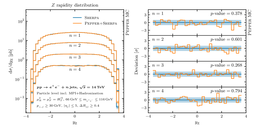
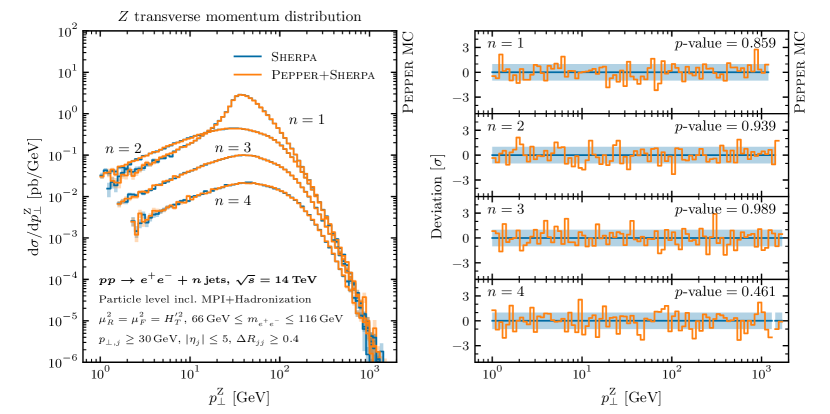
Figure 1: Particle-level validation for two observables for the $pp\to Z+n\,\text{jets}$ process, comparing Sherpa standalone results with Pepper + Sherpa results, where the parton-level events are generated by Pepper and then read in by Sherpa to perform the additional particle-level simulation. The left plots show the distributions, while the right plots show the deviations between Sherpa and Pepper + Sherpa individually for each $n$, normalized to the 1$\sigma$ standard deviation of the Sherpa result. For each $n$, the $p$-value of a Kolmogorov–Smirnov test is shown for the hypothesis that the deviations follow a standard normal distribution.

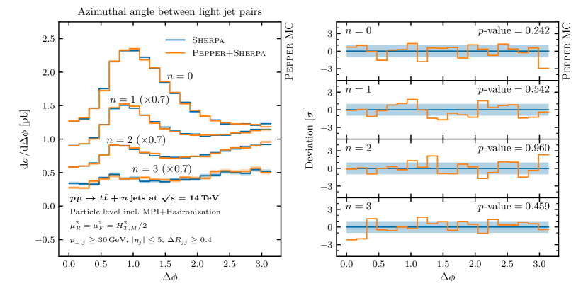
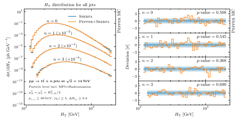
Figure 2: Particle-level validation for two observables of the $pp\to t\bar{t}+n\,\text{jets}$ process, comparing Sherpa standalone results with Pepper + Sherpa results, for which the parton-level events are generated by Pepper and then read in by Sherpa to perform the additional particle-level simulation steps. The left plots show the distributions, while the right plots show the deviations between Sherpa and Pepper + Sherpa individually for each $n$, normalized to the 1$\sigma$ standard deviation of the Sherpa result. For each $n$, the $p$-value of a Kolmogorov–Smirnov test is shown for the hypothesis that the deviations follow a standard normal distribution.

The comparison results for these two observables are shown in Fig. 1. The smaller plots shown on the right display the deviations between the results from Pepper + Sherpa and the ones from Sherpa standalone, normalized to the $1\sigma$ standard deviation of the Sherpa results. We observe agreement between the two predictions at the statistical level for all jet multiplicities.

To quantify the agreement, we test the null hypothesis that the deviations are distributed according to the standard normal using the Kolmogorov–Smirnov test [70, 71, 72]. We choose a confidence level of $95\text{\,}\mathrm{\char 37\relax}$; that is, we reject the null hypothesis (i.e. that the two distributions are identical) in favor of the alternative if the $p$-value is less than 0.05. We find that all $p$-values are greater than 0.05. The individual $p$-values are quoted in Fig. 1 for each jet multiplicity.

The second process we consider is $pp\to t\bar{t}+n\,\text{jets}$ at $\mathcal{O}(\alpha_{\rm EW}^{0})$ with $n=0,\ldots,3$. The setup is identical to the one for Drell-Yan lepton pair production, except that the renormalization and factorization scales are defined by $\mu_{R}^{2}=\mu_{F}^{2}=\mu^{2}=H_{T,M}^{2}=m_{\perp,t}^{2}+m_{\perp,\bar{t}}^{2}+\sum_{i=1}^{n}p_{\perp,i}^{2}$. The top quark decay chain is performed by Sherpa in the narrow-width approximation as described in [61]. The observables used for the validation are the azimuthal angle $\Delta\phi$ between two light jets and the $H_{T}$ of all jets, as defined in the MC_TTBAR Rivet analysis in its semi-leptonic mode.

The comparison for these two observables is shown in Fig. 2. Again, the figure on the right shows the deviations of the Pepper + Sherpa and the Sherpa standalone predictions for the different jet multiplicities, normalized to the $1\sigma$ uncertainty of the Sherpa predictions. We find agreement between the two results at the statistical level for all jet multiplicities, with the Kolmogorov–Smirnov test $p$-values all being greater than 0.05.

5 Performance

Performance benchmarks of generators for novel computing architectures in comparison to existing tools are not entirely straightforward. Differences in floating point performance, memory layout, bus performance, and other aspects of the hardware may bias any would-be one-on-one comparison. We therefore choose to analyze the code performance in two steps. First, we compare a single-threaded CPU version of Pepper to one of the event generators used at the LHC, thus establishing a baseline. We then perform a cross-platform comparison of Pepper itself. We thereby aim to demonstrate that the CPU performance of Pepper is on par with the best available algorithms, and that the underlying code is a good implementation that can easily be ported to new architectures with reasonable results.

5.1 Baseline CPU performance

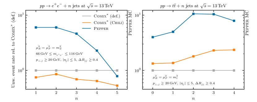
Figure 3: Event rates for generation and storage of unweighted events for $e^{+}e^{-}+n\,\text{jets}$ (left) and $t\bar{t}+n\,\text{jets}$ (right). We compare Comix, combined with its default and with the basic Chili phase-space generator, and Pepper, normalized to the Comix result. The asterisk in the Comix label indicates that the generator is used in a non-default configuration, splitting the process sum into different Monte-Carlo channels, grouping by gluons, valence and sea quarks. The results were generated on a single core of an Intel Xeon E5-2650 v2 CPU. For details, see the main text.

Figure 3 presents a comparison of the CPU version of Pepper and the parton-level event generator Comix  [73]. We measure the rate at which unweighted events are generated and stored for $e^{+}e^{-}+n\,\text{jets}$ and $t\bar{t}+n\,\text{jets}$ production at the LHC. The center-of-mass energy of the collision is set to $\sqrt{s}=13$ TeV, and the partons are required to fulfill $p_{T,j}>20$ GeV, $|\eta_{j}|<5$ and $\Delta R_{jj}>0.4$. For $e^{+}e^{-}+n\,\text{jets}$ production, an additional cut of $$66\text{\,}\mathrm{GeV}$<m_{e^{+}e^{-}}<$116\text{\,}\mathrm{GeV}$$ is applied to the invariant mass of the dilepton system. For simplicity, the renormalization and factorization scales are fixed to $\mu_{R}=\mu_{F}=m_{Z}$ in $e^{+}e^{-}+n\,\text{jets}$ production, and to $\mu_{R}=\mu_{F}=m_{t}$ in $t\bar{t}+n\,\text{jets}$ production. For better comparability of the measurements, we show Comix both in combination with its recursive phase space generator [73] and with the modified basic Chili integrator [14] that is also used by Pepper, cf. Sec. 2 for details. The raw data for Fig. 3 are listed in App. A.

For $e^{+}e^{-}+n\,\text{jets}$ production, we find that Comix combined with Chili yields a slightly reduced performance compared to Comix combined with its default phase-space integrator. As observed in [14], the Chili integrator has reduced unweighting efficiency in this case, but generates points much faster. Combining these factors results in the slightly reduced efficiency compared to the Comix default. For Pepper we observe a large throughput gain compared to Comix, especially at low multiplicities, while Comix only begins to outperform Pepper for $n=5$ additional jets. This nicely reflects the advantages of the different algorithms: The color-dressed recursion implemented in Comix adds computational overhead compared to the explicit color sum in Pepper, but the improved scaling takes over at some point. In the $t\bar{t}$+jets production, we observe a better performance of the Chili integrator comparing the two Comix results. This is also reflected in the initially increasing gain factor of Pepper when compared to the default Comix result. Despite the rather intricate color structure of the $t\bar{t}+$jets processes, Pepper outperforms Comix for all jet multiplicities tested here.

The results show that the single-threaded baseline performance of Pepper is on par with that of an existing established generator like Comix. The factorial scaling with multiplicity of the Pepper algorithm has no adverse effects in the multiplicity range of interest, where Pepper is in all cases as fast or faster than Comix. Moreover, the efficiency of the basic Chili phase-space generator used by Pepper is on par with the much more complex recursive multi-channel phase-space generator implemented in Comix, confirming earlier results [14].

5.2 Performance on different hardware

After establishing the baseline performance, we now study the suitability of Pepper for different hardware architectures. A variety of computing platforms were used to measure the portability and performance. This list defines the architecture labels used in the figures that follow:

2$\times$Skylake8180

Intel Xeon Platinum 8180M CPU at 2.50 GHz with $768\text{\,}\mathrm{G}\mathrm{B}$ of memory. These are 28-core processors; and the machine contains two CPUs each. Our performance tests utilize all 56 cores unless otherwise noted, hence the “$2\times$” in our label.

V100

Nvidia V100(SXM2) GPU with $32\text{\,}\mathrm{G}\mathrm{B}$ of memory.

A100

Nvidia A100 GPU with $40\text{\,}\mathrm{G}\mathrm{B}$ of memory. Similar to the Perlmutter (113 Pflop/s) [74], Leonardo (304 PFlop/s) [75] and JUWELS (70 Pflop/s) [76] systems.

H100

Nvidia H100 GPU with $80\text{\,}\mathrm{G}\mathrm{B}$ of memory. This is a recent release by Nvidia and a likely target for next generation supercomputers.

MI100

AMD MI100 GPU with $32\text{\,}\mathrm{G}\mathrm{B}$ of memory.

$\mathbf{\nicefrac{{1}}{{2}}\times}$MI250

AMD MI250 GPU with $32\text{\,}\mathrm{G}\mathrm{B}$ of memory. Similar to the Frontier (1.6 Eflop/s) [77], LUMI (531 Pflop/s) [78] and Adastra (61 Pflop/s) [79] systems. Each GPU has two tiles. In Pepper, each tile acts as an independent device. Therefore we choose to utilize a single tile for our performance tests, which is why we include “$\nicefrac{{1}}{{2}}\times$” in our label.

PVC

Intel Data Center GPU Max Series with $128\text{\,}\mathrm{G}\mathrm{B}$ of memory. This is part of the Sunspot testbed [80] of the Aurora (1.0Eflop/s) systems [81]. Sunspot is a pre-production supercomputer with early versions of the Aurora software development kit.

Using a portability framework like Kokkos in the Pepper event generator is a novel feature for a production-ready parton-level event generator, and for much of the HEP software stack in general. We have therefore tested the performance of the Kokkos Pepper variant against the native CUDA and the native single-threaded CPU variants, on an A100 GPU and an Intel Core i3-8300 CPU at 3.70 GHz CPU, respectively. Comparing the event throughput, we find that the performance of the Kokkos variant agrees within less than a factor of two with the performance of the native variants when compared on the same hardware, with the native variants being better in most cases. This result establishes that using a portability framework is possible without compromising significantly on performance, while at the same time giving access to a much wider range of architectures and computing paradigms. With that, we only show Kokkos result in the following. We note, however, that our current Kokkos implementation on the CPU does not utilize vectorization capabilities. We have constructed a vectorized version of out native C++ implementation with the help of the VCL library [82], which shows that significant speedups can be achieved on the CPU. Because the focus of the analysis here is on portability, these improvements are not yet included in Figs. 4 and 5. We expect to provide a Kokkos implementation with vectorization capabilities in the future.

First we study the performance on different architectures for the evaluation of weighted parton-level $gg\to t\bar{t}+ng$ events for $n=0,\ldots,5$ at a fixed centre-of-mass energy, thus testing the matrix element throughput of Pepper in a wide range of parton multiplicity. The results are shown in Fig. 4. We find that Pepper achieves at least an order of magnitude higher throughput on the H100 GPU than on two 28-core Skylake CPUs. The results for the other accelerators lie between the H100 and the 2$\times$Skylake8180 result. The performance on MI100/250 scales slightly worse than the NVidia GPU with the number of additional gluons and thus with the memory footprint of the algorithm, but overall the scaling with multiplicity is qualitatively similar on all architectures. The results show that Pepper’s matrix-element evaluation is successfully ported to a wide range of hardware from different vendors.

Our next test addresses the generation of full parton-level events including unweighting, event write-out and partonic fluxes in $pp\to e^{+}e^{-}+n\,\text{jets}$and $pp\to t\bar{t}+n\,\text{jets}$. The event rates are presented in Fig. 5. The numeric results are tabulated for reference in App. A. Overall, the results are similar to the ones presented in Fig. 4. One difference is that the event rates are more on par for very low multiplicities $n=0,1$. This is because the output of the events becomes the dominant part of the simulation due to the high phase-space efficiency and the very large matrix-element throughput on GPUs. Details are discussed in App. B. Ignoring the lowest two multiplicities, we find that the H100 event rates are 20 to 50 times higher than the 2$\times$Skylake8180 ones. Another difference to the matrix element only case is that the scaling with multiplicity is steeper due to the quickly decreasing unweighting efficiencies. Again, the scaling is similar on all architectures. These results show that the entire Pepper pipeline of parton-level event generation and writeout is successfully ported to a wide range of hardware.

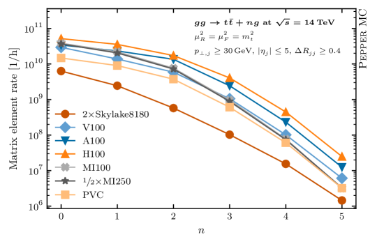
Figure 4: Comparison of the throughput achieved for the $gg\to t\bar{t}+ng$ process for the matrix element evaluation on different computing architectures. For details, see the main text.

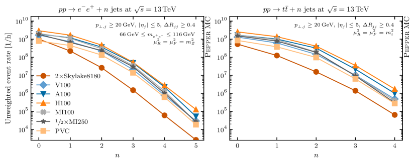
Figure 5: Comparison of the unweighted event generation and storage rates achieved for the $pp\to e^{+}e^{-}+n\,\text{jets}$ (left) and $pp\to t\bar{t}+n\,\text{jets}$ (right) processes on different computing architectures. For details, see the main text.

5.3 Scaling to many nodes

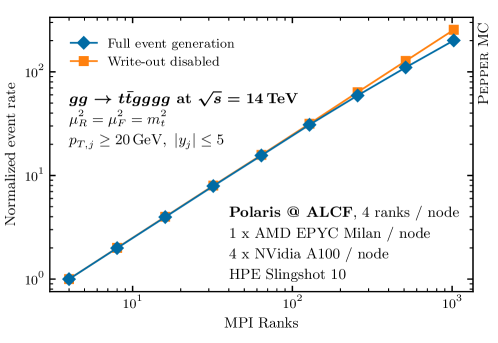
Figure 6: Scaling test of Pepper event generation on the Polaris system [83] at ALCF. The event rates for the $gg\to t\bar{t}gggg$ process are shown, normalized to the rate on 4 MPI ranks. See the main text for details.

Finally, we perform a weak scaling test of Pepper on the Polaris system at ALCF [83]. Polaris is a testbed to prepare applications and workloads for science in the exascale era and consists of 560 nodes with one AMD EPYC Milan processor and four NVidia A100 GPUs each. The nodes have unified memory architecture and two fabric endpoints, the system interconnect is a HPE Slingshot 10 network at the time of our study. For our test, we hold the number of generated events per node constant and increase the number of nodes. We measure the number of unweighted events in $gg\to t\bar{t}gggg$ production. The gluon flux is evaluated using the Lhapdf library with its builtin MPI support enabled. Figure 6 shows the event rate as a function of the number of MPI ranks, normalized to the rate on a single node. Here the number of MPI ranks is equal to the number of GPUs. We notice that the scaling is violated starting from about 512 ranks. However, we observe that the scaling violation is entirely due to the event output via the HDF5 library. We expect to be able to alleviate this problem in the future through performance tuning of HDF5, similar to the effort reported in [32].

6 Summary and Outlook

Pepper is the first complete framework to reach production-level quality in parton-level event generation for collider physics on different computing architectures. It includes matrix-element calculation, phase-space integration, PDF evaluation, and processing of the events for storage in event files. This development marks a major milestone identified by the generator working group of the HEP Software Foundation [3, 4] and by the HEP Center for Computational Excellence [84]. It frees up valuable CPU resources for the analysis of experimental data at the Large Hadron Collider. Parton-level event generation will now no longer contribute to the projected shortfall in computing resources during Run 4 and 5 and the high-luminosity phase of the LHC. In addition, we enable the Large Hadron Collider experiments to utilize most available (pre-)exascale computing facilities, which is an important step towards a sustainable computing model for the future of collider phenomenology.

The Pepper event generator is ready for production-level use in many processes to be simulated at high fidelity at the LHC, i.e. $\ell^{+}\ell^{-}+$jets, $t\bar{t}+$jets, pure jets and multiple heavy quark production (e.g. $bb\bar{b}\bar{b}+$jets or $t\bar{t}b\bar{b}+$jets). The combination with the particle-level event generation framework in [14] makes it possible to process events with Pythia 8 [62] or Sherpa 2 [61]. An extension of Pepper to processes such as $\ell\bar{\nu}_{\ell}+$jets, $VV+$jets, $\gamma\gamma+$jets and to other reactions with high computing demands will become available in the short term. The compute performance of the CPU version of Pepper is better than that of Comix, one of the leading and most widely used automated matrix element generators for the LHC. We have shown, for a variety of architectures, that Pepper can efficiently generate parton-level events, and we have demonstrated scalability up to 512 NVidia A100 GPUs on the Polaris system at ALCF.

Appendix A Tabulated performance results

Table 1 lists the baseline performance data shown graphically in Fig. 3. While the figure shows ratios, we list here the absolute event rates found for Comix and Pepper using single-threaded execution. For additional details, see Sec. 5.1.

Events / hour	Comix∗		Pepper
	Comix	Chili
$pp\to e^{+}e^{-}+1j$	1.2e7	9.0e6	7.2e7
$pp\to e^{+}e^{-}+2j$	1.2e6	1.0e6	7.2e6
$pp\to e^{+}e^{-}+3j$	1.1e5	7.5e4	5.0e5
$pp\to e^{+}e^{-}+4j$	6.2e3	4.0e3	1.4e4
$pp\to e^{+}e^{-}+5j$	3.8e2	2.0e2	3.0e2

Events / hour	Comix∗		Pepper
	Comix	Chili
$pp\to t\bar{t}+0j$	9.0e6	1.2e7	3.6e7
$pp\to t\bar{t}+1j$	2.4e6	3.3e6	1.2e7
$pp\to t\bar{t}+2j$	2.1e5	3.8e5	2.2e6
$pp\to t\bar{t}+3j$	1.2e4	2.9e4	1.3e5
$pp\to t\bar{t}+4j$	8.1e2	1.9e3	6.4e3

Table 1: Comparison of the event rates achieved for $pp\to e^{+}e^{-}+n\,\text{jets}$ (left) and $pp\to t\bar{t}+n\,\text{jets}$ (right) by Comix, combined with its default and with the basic Chili phase-space generator, and Pepper. The asterisk in the Comix label indicates that it is run in a non-default but more efficient mode, splitting the process sum into different Monte-Carlo channels, grouping by gluons, valence and sea quarks. The results were generated on a single core of an Intel Xeon E5-2650 v2 CPU. For details, see Sec. 5.1.

Table 2 lists the unweighted events rates on different computing architectures. This is the raw data for Fig. 5. For additional details, see Sec. 5.2.

Events / hour	2$\times$Skylake8180	V100	A100	H100	MI100	$\nicefrac{{1}}{{2}}\times$MI250	PVC
$pp\to t\bar{t}+0j$	5.3e8	1.3e9	1.7e9	2.5e9	1.6e9	1.5e9	8.5e8
$pp\to t\bar{t}+1j$	1.2e8	6.2e8	1.0e9	1.4e9	9.4e8	7.8e8	3.8e8
$pp\to t\bar{t}+2j$	1.6e7	1.4e8	3.2e8	4.1e8	1.9e8	1.9e8	9.7e7
$pp\to t\bar{t}+3j$	1.4e6	1.0e7	2.2e7	3.5e7	9.4e6	9.2e6	6.3e6
$pp\to t\bar{t}+4j$	6.4e4	4.8e5	1.0e6	1.7e6	4.0e5	3.0e5	2.8e5
$pp\to e^{-}e^{+}+0j$	1.0e9	1.7e9	1.9e9	2.9e9	2.1e9	1.8e9	7.9e8
$pp\to e^{-}e^{+}+1j$	2.2e8	7.3e8	1.2e9	1.7e9	1.1e9	6.6e8	4.5e8
$pp\to e^{-}e^{+}+2j$	2.6e7	2.2e8	3.6e8	4.7e8	2.9e8	2.3e8	1.3e8
$pp\to e^{-}e^{+}+3j$	1.5e6	2.1e7	4.8e7	5.2e7	3.4e7	3.0e7	1.4e7
$pp\to e^{-}e^{+}+4j$	6.0e4	7.8e5	2.2e6	2.7e6	1.3e6	1.0e6	6.1e5
$pp\to e^{-}e^{+}+5j$	2.6e3	2.9e4	5.3e4	1.3e5	2.5e4	2.7e4	1.8e4

Table 2: Comparison of the unweighted event generation (and storage) rates achieved for the $pp\to t\bar{t}+n\,\text{jets}$ and $pp\to e^{+}e^{-}+n\,\text{jets}$ processes on different architectures.

Appendix B Runtime distribution

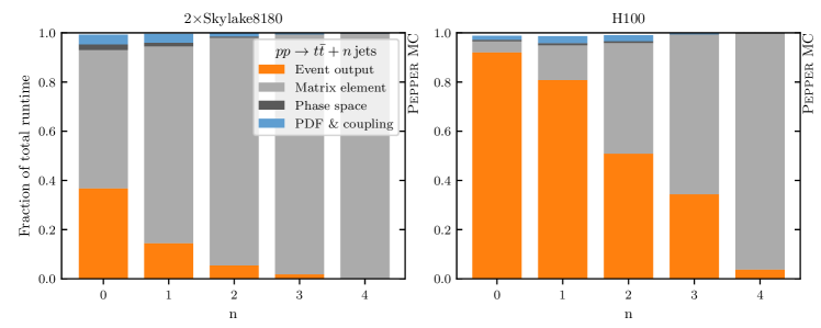
Figure 7: The fraction of event generation runtime spent on different components of the pipeline, for the $pp\to t\bar{t}+n\,\text{jets}$ process. On the left, we show the data for the 2$\times$Skylake8180 CPU, while on the right we show it for the NVidia H100 GPU. The components are Event Output, Matrix element evaluation, Phase space sampling, and PDF and strong coupling evaluation.

In Sec. 5.2, we found that the event rates for the lowest multiplicities are comparably similar across the different computing architectures, see Fig. 5. To understand this better, we plot the fractions of computing time spent in different components of the event generation in Fig. 7. The different components studied are the Berends–Giele recursion for the matrix element evaluation, the event output, the evaluation of the strong coupling and partonic fluxes, and the phase space generation. On the left side we plot the data of the 2$\times$Skylake8180 architecture, while on the right side we plot the data of the NVidia H100 architecture. These are representative of a (two-chip) CPU system and a GPU architecture. While on the CPU the majority of time is always spent on the matrix element evaluation, we have a different situation on the GPU. Here, for the lowest three multiplicities the majority of time is spent on the event output. This is because the matrix element evaluation rate on the GPU is so high that the overall rate is now constrained by the event file write-out. However, in the current implementation of GPU write-out, only a single CPU core is used. Therefore, the write-out rate could be improved by utilizing the idle CPUs on each node, an implementation of this procedure is left to a future version of Pepper.

References

- [1] A. Buckley et al., General-purpose event generators for LHC physics, Phys. Rept. 504, 145 (2011), 10.1016/j.physrep.2011.03.005, 1101.2599.
- [2] J. M. Campbell et al., Event Generators for High-Energy Physics Experiments, In Snowmass 2021 (2022), 2203.11110.
- [3] S. Amoroso et al., Challenges in Monte Carlo Event Generator Software for High-Luminosity LHC, Comput. Softw. Big Sci. 5(1), 12 (2021), 10.1007/s41781-021-00055-1, 2004.13687.
- [4] E. Yazgan et al., HL-LHC Computing Review Stage-2, Common Software Projects: Event Generators (2021), 2109.14938.
- [5] P. Skands, Computational scientists should consider climate impacts and grant agencies should reward them, Nature Rev. Phys. 5(3), 137 (2023), 10.1038/s42254-023-00563-6.
- [6] O. Mattelaer and K. Ostrolenk, Speeding up MadGraph5_aMC@NLO, Eur. Phys. J. C 81(5), 435 (2021), 10.1140/epjc/s10052-021-09204-7, 2102.00773.
- [7] E. Bothmann, A. Buckley, I. A. Christidi, C. Gütschow, S. Höche, M. Knobbe, T. Martin and M. Schönherr, Accelerating LHC event generation with simplified pilot runs and fast PDFs, Eur. Phys. J. C 82(12), 1128 (2022), 10.1140/epjc/s10052-022-11087-1, 2209.00843.
- [8] E. Bothmann, T. Janßen, M. Knobbe, T. Schmale and S. Schumann, Exploring phase space with Neural Importance Sampling, SciPost Phys. 8(4), 069 (2020), 10.21468/SciPostPhys.8.4.069, 2001.05478.
- [9] C. Gao, J. Isaacson and C. Krause, i-flow: High-dimensional Integration and Sampling with Normalizing Flows, Mach. Learn. Sci. Tech. 1(4), 045023 (2020), 10.1088/2632-2153/abab62, 2001.05486.
- [10] C. Gao, S. Höche, J. Isaacson, C. Krause and H. Schulz, Event Generation with Normalizing Flows, Phys. Rev. D 101(7), 076002 (2020), 10.1103/PhysRevD.101.076002, 2001.10028.
- [11] T. Heimel, R. Winterhalder, A. Butter, J. Isaacson, C. Krause, F. Maltoni, O. Mattelaer and T. Plehn, MadNIS - Neural multi-channel importance sampling, SciPost Phys. 15(4), 141 (2023), 10.21468/SciPostPhys.15.4.141, 2212.06172.
- [12] S. Badger et al., Machine learning and LHC event generation, SciPost Phys. 14(4), 079 (2023), 10.21468/SciPostPhys.14.4.079, 2203.07460.
- [13] T. Heimel, N. Huetsch, F. Maltoni, O. Mattelaer, T. Plehn and R. Winterhalder, The MadNIS Reloaded (2023), 2311.01548.
- [14] E. Bothmann, T. Childers, W. Giele, F. Herren, S. Hoeche, J. Isaacson, M. Knobbe and R. Wang, Efficient phase-space generation for hadron collider event simulation, SciPost Phys. 15(4), 169 (2023), 10.21468/SciPostPhys.15.4.169, 2302.10449.
- [15] R. Frederix, S. Frixione, S. Prestel and P. Torrielli, On the reduction of negative weights in MC@NLO-type matching procedures, JHEP 07, 238 (2020), 10.1007/JHEP07(2020)238, 2002.12716.
- [16] K. Danziger, S. Höche and F. Siegert, Reducing negative weights in Monte Carlo event generation with Sherpa (2021), 2110.15211.
- [17] J. M. Campbell, S. Höche and C. T. Preuss, Accelerating LHC phenomenology with analytic one-loop amplitudes: A C++ interface to MCFM, Eur. Phys. J. C 81(12), 1117 (2021), 10.1140/epjc/s10052-021-09885-0, 2107.04472.
- [18] K. Danziger, T. Janßen, S. Schumann and F. Siegert, Accelerating Monte Carlo event generation – rejection sampling using neural network event-weight estimates, SciPost Phys. 12, 164 (2022), 10.21468/SciPostPhys.12.5.164, 2109.11964.
- [19] D. Maître and H. Truong, A factorisation-aware Matrix element emulator, JHEP 11, 066 (2021), 10.1007/JHEP11(2021)066, 2107.06625.
- [20] D. Maître and H. Truong, One-loop matrix element emulation with factorisation awareness (2023), 10.1007/JHEP05(2023)159, 2302.04005.
- [21] T. Janßen, D. Maître, S. Schumann, F. Siegert and H. Truong, Unweighting multijet event generation using factorisation-aware neural networks, SciPost Phys. 15(3), 107 (2023), 10.21468/SciPostPhys.15.3.107, 2301.13562.
- [22] W. Giele, G. Stavenga and J.-C. Winter, Thread-Scalable Evaluation of Multi-Jet Observables, Eur. Phys. J. C 71, 1703 (2011), 10.1140/epjc/s10052-011-1703-5, 1002.3446.
- [23] K. Hagiwara, J. Kanzaki, N. Okamura, D. Rainwater and T. Stelzer, Calculation of HELAS amplitudes for QCD processes using graphics processing unit (GPU), Eur. Phys. J. C 70, 513 (2010), 10.1140/epjc/s10052-010-1465-5, 0909.5257.
- [24] K. Hagiwara, J. Kanzaki, N. Okamura, D. Rainwater and T. Stelzer, Fast calculation of HELAS amplitudes using graphics processing unit (GPU), Eur. Phys. J. C 66, 477 (2010), 10.1140/epjc/s10052-010-1276-8, 0908.4403.
- [25] K. Hagiwara, J. Kanzaki, Q. Li, N. Okamura and T. Stelzer, Fast computation of MadGraph amplitudes on graphics processing unit (GPU), Eur. Phys. J. C 73, 2608 (2013), 10.1140/epjc/s10052-013-2608-2, 1305.0708.
- [26] E. Bothmann, W. Giele, S. Höche, J. Isaacson and M. Knobbe, Many-gluon tree amplitudes on modern GPUs: A case study for novel event generators (2021), 10.21468/SciPostPhysCodeb.3, 2106.06507.
- [27] A. Valassi, S. Roiser, O. Mattelaer and S. Hageböck, Design and engineering of a simplified workflow execution for the MG5aMC event generator on GPUs and vector CPUs, EPJ Web Conf. 251, 03045 (2021), 10.1051/epjconf/202125103045, 2106.12631.
- [28] A. Valassi, T. Childers, L. Field, S. Hageböck, W. Hopkins, O. Mattelaer, N. Nichols, S. Roiser and D. Smith, Developments in Performance and Portability for MadGraph5_aMC@NLO, PoS ICHEP2022, 212 (2022), 10.22323/1.414.0212, 2210.11122.
- [29] E. Bothmann, J. Isaacson, M. Knobbe, S. Höche and W. Giele, QCD tree amplitudes on modern GPUs: A case study for novel event generators, PoS ICHEP2022, 222 (2022), 10.22323/1.414.0222.
- [30] A. Valassi et al., Speeding up Madgraph5 aMC@NLO through CPU vectorization and GPU offloading: towards a first alpha release, In 21th International Workshop on Advanced Computing and Analysis Techniques in Physics Research: AI meets Reality (2023), 2303.18244.
- [31] S. Höche, S. Prestel and H. Schulz, Simulation of Vector Boson Plus Many Jet Final States at the High Luminosity LHC, Phys. Rev. D100(1), 014024 (2019), 10.1103/PhysRevD.100.014024, 1905.05120.
- [32] E. Bothmann, T. Childers, C. Gütschow, S. Höche, P. Hovland, J. Isaacson, M. Knobbe and R. Latham, Efficient precision simulation of processes with many-jet final states at the LHC (2023), 2309.13154.
- [33] F. Berends and W. Giele, The six-gluon process as an example of weyl-van der waerden spinor calculus, Nuclear Physics B 294, 700 (1987), https://doi.org/10.1016/0550-3213(87)90604-3.
- [34] V. Del Duca, A. Frizzo and F. Maltoni, Factorization of tree QCD amplitudes in the high-energy limit and in the collinear limit, Nucl. Phys. B 568, 211 (2000), 10.1016/S0550-3213(99)00657-4, hep-ph/9909464.
- [35] V. Del Duca, L. J. Dixon and F. Maltoni, New color decompositions for gauge amplitudes at tree and loop level, Nucl. Phys. B 571, 51 (2000), 10.1016/S0550-3213(99)00809-3, hep-ph/9910563.
- [36] T. Melia, Dyck words and multiquark primitive amplitudes, Phys. Rev. D 88(1), 014020 (2013), 10.1103/PhysRevD.88.014020, 1304.7809.
- [37] T. Melia, Dyck words and multi-quark amplitudes, PoS RADCOR2013, 031 (2013), 10.22323/1.197.0031.
- [38] H. Johansson and A. Ochirov, Color-Kinematics Duality for QCD Amplitudes, JHEP 01, 170 (2016), 10.1007/JHEP01(2016)170, 1507.00332.
- [39] T. Melia, Proof of a new colour decomposition for QCD amplitudes, JHEP 12, 107 (2015), 10.1007/JHEP12(2015)107, 1509.03297.
- [40] M. Dinsdale, M. Ternick and S. Weinzierl, A Comparison of efficient methods for the computation of Born gluon amplitudes, JHEP 03, 056 (2006), 10.1088/1126-6708/2006/03/056, hep-ph/0602204.
- [41] C. Duhr, S. Höche and F. Maltoni, Color-dressed recursive relations for multi-parton amplitudes, JHEP 08, 062 (2006), 10.1088/1126-6708/2006/08/062, hep-ph/0607057.
- [42] S. Badger, B. Biedermann, L. Hackl, J. Plefka, T. Schuster and P. Uwer, Comparing efficient computation methods for massless QCD tree amplitudes: Closed analytic formulas versus Berends-Giele recursion, Phys. Rev. D 87(3), 034011 (2013), 10.1103/PhysRevD.87.034011, 1206.2381.
- [43] F. Berends and W. Giele, Recursive calculations for processes with n gluons, Nuclear Physics B 306(4), 759 (1988), https://doi.org/10.1016/0550-3213(88)90442-7.
- [44] F. A. Berends, W. T. Giele and H. Kuijf, Exact Expressions for Processes Involving a Vector Boson and Up to Five Partons, Nucl. Phys. B 321, 39 (1989), 10.1016/0550-3213(89)90242-3.
- [45] F. A. Berends, H. Kuijf, B. Tausk and W. T. Giele, On the production of a W and jets at hadron colliders, Nucl. Phys. B 357, 32 (1991), 10.1016/0550-3213(91)90458-A.
- [46] E. Byckling and K. Kajantie, N-particle phase space in terms of invariant momentum transfers, Nucl. Phys. B 9, 568 (1969), 10.1016/0550-3213(69)90271-5.
- [47] F. James, Monte-Carlo phase space (1968).
- [48] A. Buckley, J. Ferrando, S. Lloyd, K. Nordström, B. Page, M. Rüfenacht, M. Schönherr and G. Watt, LHAPDF6: parton density access in the LHC precision era, Eur. Phys. J. C 75, 132 (2015), 10.1140/epjc/s10052-015-3318-8, 1412.7420.
- [49] R. Kleiss and R. Pittau, Weight optimization in multichannel Monte Carlo, Comput. Phys. Commun. 83, 141 (1994), 10.1016/0010-4655(94)90043-4, hep-ph/9405257.
- [50] M. L. Mangano and S. J. Parke, Multiparton amplitudes in gauge theories, Phys. Rept. 200, 301 (1991), 10.1016/0370-1573(91)90091-Y, hep-th/0509223.
- [51] H. Carter Edwards , Christian R. Trott , Daniel Sunderland, Kokkos: Enabling manycore performance portability through polymorphic memory access patterns, JPDC 74, 3202 (2014), https://doi.org/10.1016/j.jpdc.2014.07.003.
- [52] C. R. Trott, D. Lebrun-Grandié, D. Arndt, J. Ciesko, V. Dang, N. Ellingwood, R. Gayatri, E. Harvey, D. S. Hollman, D. Ibanez, N. Liber, J. Madsen et al., Kokkos 3: Programming model extensions for the exascale era, IEEE Transactions on Parallel and Distributed Systems 33(4), 805 (2022), 10.1109/TPDS.2021.3097283.
- [53] Message Passing Interface Forum, MPI: A Message-Passing Interface Standard Version 4.0 (2021).
- [54] A. Buckley, P. Ilten, D. Konstantinov, L. Lönnblad, J. Monk, W. Pokorski, T. Przedzinski and A. Verbytskyi, The HepMC3 event record library for Monte Carlo event generators, Comput. Phys. Commun. 260, 107310 (2021), 10.1016/j.cpc.2020.107310, 1912.08005.
- [55] C. Bierlich et al., Robust Independent Validation of Experiment and Theory: Rivet version 3, SciPost Phys. 8, 026 (2020), 10.21468/SciPostPhys.8.2.026, 1912.05451.
- [56] J. Alwall et al., A Standard format for Les Houches event files, Comput. Phys. Commun. 176, 300 (2007), 10.1016/j.cpc.2006.11.010, hep-ph/0609017.
- [57] J. R. Andersen et al., Les Houches 2013: Physics at TeV Colliders: Standard Model Working Group Report (2014), 1405.1067.
- [58] The HDF Group, Hierarchical Data Format, version 5, https://www.hdfgroup.org/HDF5/.
- [59] HighFive - HDF5 header-only C++ Library, https://bluebrain.github.io/HighFive/.
- [60] T. Gleisberg, S. Höche, F. Krauss, M. Schönherr, S. Schumann, F. Siegert and J. Winter, Event generation with SHERPA 1.1, JHEP 02, 007 (2009), 10.1088/1126-6708/2009/02/007, 0811.4622.
- [61] E. Bothmann et al., Event Generation with Sherpa 2.2, SciPost Phys. 7(3), 034 (2019), 10.21468/SciPostPhys.7.3.034, 1905.09127.
- [62] T. Sjöstrand, S. Ask, J. R. Christiansen, R. Corke, N. Desai, P. Ilten, S. Mrenna, S. Prestel, C. O. Rasmussen and P. Z. Skands, An introduction to PYTHIA 8.2, Comput. Phys. Commun. 191, 159 (2015), 10.1016/j.cpc.2015.01.024, 1410.3012.
- [63] C. Bierlich et al., A comprehensive guide to the physics and usage of PYTHIA 8.3 (2022), 10.21468/SciPostPhysCodeb.8, 2203.11601.
- [64] F. Krauss, R. Kuhn and G. Soff, AMEGIC++ 1.0: A Matrix element generator in C++, JHEP 02, 044 (2002), 10.1088/1126-6708/2002/02/044, hep-ph/0109036.
- [65] S. Schumann and F. Krauss, A Parton shower algorithm based on Catani-Seymour dipole factorisation, JHEP 03, 038 (2008), 10.1088/1126-6708/2008/03/038, 0709.1027.
- [66] J.-C. Winter, F. Krauss and G. Soff, A Modified cluster hadronization model, Eur. Phys. J. C 36, 381 (2004), 10.1140/epjc/s2004-01960-8, hep-ph/0311085.
- [67] T. Sjöstrand and M. van Zijl, A Multiple Interaction Model for the Event Structure in Hadron Collisions, Phys. Rev. D 36, 2019 (1987), 10.1103/PhysRevD.36.2019.
- [68] A. De Roeck and H. Jung, eds., HERA and the LHC: A Workshop on the implications of HERA for LHC physics: Proceedings Part A, CERN Yellow Reports: Conference Proceedings. CERN, Geneva, 10.5170/CERN-2005-014 (2005), hep-ph/0601012.
- [69] R. D. Ball et al., Parton distributions for the LHC Run II, JHEP 04, 040 (2015), 10.1007/JHEP04(2015)040, 1410.8849.
- [70] K. AN, Sulla determinazione empirica di una legge didistribuzione, Giorn Dell’inst Ital Degli Att 4, 89 (1933).
- [71] N. V. Smirnov, On the estimation of the discrepancy between empirical curves of distribution for two independent samples, Bull. Math. Univ. Moscou 2(2), 3 (1939).
- [72] F. J. Massey, Distribution table for the deviation between two sample cumulatives, The annals of mathematical statistics 23(3), 435 (1952).
- [73] T. Gleisberg and S. Höche, Comix, a new matrix element generator, JHEP 12, 039 (2008), 10.1088/1126-6708/2008/12/039, 0808.3674.
- [74] Perlmutter computing system at NERSC, https://www.nersc.gov/systems/perlmutter.
- [75] Leonardo computing system at CINECA, https://leonardo-supercomputer.cineca.eu.
- [76] JUWELS computing system at FZ Jülich, https://www.fz-juelich.de/en/ias/jsc/systems/supercomputers/juwels.
- [77] Frontier computing system at OLCF, https://www.olcf.ornl.gov/frontier.
- [78] LUMI computing systema at EuroHPC JU, https://lumi-supercomputer.eu.
- [79] Adastra computing system at GENCI, https://genci.link/en/centre-informatique-national-de-lenseignement-superieur-cines.
- [80] Sunspot testbed at ALCF, https://www.alcf.anl.gov/news/argonne-s-new-sunspot-testbed-provides-ramp-aurora-exascale-supercomputer.
- [81] Aurora computing system at ALCF, https://www.alcf.anl.gov/aurora.
- [82] Agner Fog, Vector Class Library, https://github.com/vectorclass/.
- [83] Polaris testbed at ALCF, https://www.alcf.anl.gov/polaris.
- [84] High-Energy Physics Center for Computational Excellence, https://www.anl.gov/hep-cce.